Revisiting the Importance of Encoding Logic Rules in Sentiment Classification

4743

Revisiting the Importance of Encoding Logic Rules

in Sentiment Classification

Kalpesh Krishna♠♣ Preethi Jyothi♠

Indian Institute of Technology, Bombay♠ University of Massachusetts, Amherst♣

{kalpesh,miyyer}@cs.umass.edu [email protected]

Mohit Iyyer♣

Abstract

We analyze the performance of different sen-timent classification models on syntactically-complex inputs likeA-but-B sentences. The first contribution of this analysis addresses re-producible research: to meaningfully compare different models, their accuracies must be av-eraged over far more random seeds than what has traditionally been reported. With proper averaging in place, we notice that the distil-lation model described in Hu et al. (2016), which incorporates explicit logic rules for sen-timent classification, is ineffective. In contrast, using contextualized ELMo embeddings ( Pe-ters et al.,2018a) instead of logic rules yields significantly better performance. Additionally, we provide analysis and visualizations that demonstrate ELMo’s ability to implicitly learn logic rules. Finally, a crowdsourced analysis reveals how ELMo outperforms baseline mod-els even on sentences with ambiguous senti-ment labels.

1 Introduction

In this paper, we explore the effectiveness of meth-ods designed to improve sentiment classification (positive vs. negative) of sentences that con-tain complex syntactic structures. While simple bag-of-words or lexicon-based methods (Pang and Lee,2005;Wang and Manning,2012;Iyyer et al.,

2015) achieve good performance on this task, they are unequipped to deal with syntactic structures that affect sentiment, such as contrastive conjunc-tions (i.e., sentences of the form “A-but-B”) or negations. Neural models that explicitly encode word order (Kim, 2014), syntax (Socher et al.,

2013;Tai et al., 2015) and semantic features (Li et al., 2017) have been proposed with the aim of improving performance on these more compli-cated sentences. Recently, Hu et al. (2016) in-corporate logical rules into a neural model and

show that these rules increase the model’s accu-racy on sentences containing contrastive conjunc-tions, whilePeters et al.(2018a) demonstrate in-creased overall accuracy on sentiment analysis by initializing a model with representations from a language model trained on millions of sentences.

In this work, we carry out an in-depth study of the effectiveness of the techniques inHu et al.

(2016) andPeters et al.(2018a) for sentiment clas-sification of complex sentences. Part of our con-tribution is to identify an important gap in the methodology used inHu et al. (2016) for perfor-mance measurement, which is addressed by av-eraging the experiments over several executions. With the averaging in place, we obtain three key findings: (1) the improvements inHu et al.(2016) can almost entirely be attributed to just one of their two proposed mechanisms and are also less pronounced than previously reported; (2) contex-tualized word embeddings (Peters et al., 2018a) incorporate the “A-but-B” rules more effectively without explicitly programming for them; and (3) an analysis using crowdsourcing reveals a big-ger picture where the errors in the automated sys-tems have a striking correlation with the inherent sentiment-ambiguity in the data.

2 Logic Rules in Sentiment Classification

Here we briefly review background fromHu et al.

(2016) to provide a foundation for our reanalysis in the next section. We focus on a logic rule for sentences containing an “A-but-B”structure (the only rule for whichHu et al.(2016) provide exper-imental results). Intuitively, the logic rule for such sentences is that the sentiment associated with the whole sentence should be the same as the senti-ment associated with phrase“B”.1

More formally, let pθ(y|x) denote the

proba-bility assigned to the label y ∈ {+,−} for an input x by the baseline model using parameters θ. A logic rule is (softly) encoded as a variable rθ(x, y) ∈ [0,1] indicating how well labeling x

with y satisfies the rule. For the case ofA-but-B sentences,rθ(x, y) = pθ(y|B)ifxhas the

struc-tureA-but-B (and 1 otherwise). Next, we discuss the two techniques from Hu et al. (2016) for in-corporating rules into models: projection, which directly alters a trained model, and distillation, which progressively adjusts the loss function dur-ing traindur-ing.

Projection. The first technique is to project a trained model into a rule-regularized subspace, in a fashion similar toGanchev et al. (2010). More precisely, a given modelpθis projected to a model

qθ defined by the optimum value ofq in the

fol-lowing optimization problem:2

min

q,ξ≥0KL(q(X, Y)||pθ(X, Y)) +C

X

x∈X

ξx

s.t. (1−_Ey←q(·|x)[rθ(x, y)])≤ξx

Here q(X, Y) denotes the distribution of (x, y)

when x is drawn uniformly from the set X and yis drawn according toq(·|x).

Iterative Rule Knowledge Distillation. The second technique is to transfer the domain knowl-edge encoded in the logic rules into a neural network’s parameters. Following Hinton et al.

(2015), a “student” model pθ can learn from

the “teacher” model qθ, by using a loss function

πH(pθ, Ptrue) + (1−π)H(pθ, qθ)during training,

where Ptrue denotes the distribution implied by

the ground truth,H(·,·)denotes the cross-entropy function, and π is a hyperparameter. Hu et al.

(2016) computes qθ after every gradient update

by projecting the current pθ, as described above.

Note that both mechanisms can be combined: Af-ter fully trainingpθ using the iterative distillation

process above, the projection step can be applied one more time to obtainqθ which is then used as

the trained model.

Dataset. All of our experiments (as well as those in Hu et al. (2016)) use the SST2 dataset, a

2_{The formulation inHu et al.(2016) includes another} hy-perparameterλper rule, to control its relative importance; when there is only one rule, as in our case, this parameter can be absorbed intoC.

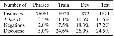
binarized subset of the popular Stanford Senti-ment Treebank (SST) (Socher et al., 2013). The dataset includes phrase-level labels in addition to sentence-level labels (see Table 1 for detailed statistics); followingHu et al.(2016), we use both types of labels for the comparisons inSection 3.2. In all other experiments, we use only sentence-level labels, and our baseline model for all exper-iments is the CNN architecture fromKim(2014).

3 A Reanalysis

In this section we reanalyze the effectiveness of the techniques of Hu et al. (2016) and find that most of the performance gain is due to projection and not knowledge distillation. The discrepancy with the original analysis can be attributed to the relatively small dataset and the resulting variance across random initializations. We start by analyz-ing the baseline CNN byKim(2014) to point out the need for an averaged analysis.

0.0 0.2 0.4 0.6

83.47 85.64 86.16 86.49 87.20

Accuracy (%)

Number of epochs of training

Figure 1: Variation in models trained on SST-2 (sentence-only). Accuracies of 100 randomly initialized models are plotted against the number of epochs of training (in gray), along with their average accuracies (in red, with 95% confi-dence interval error bars). The inset density plot shows the distribution of accuracies when trained with early stopping.

3.1 Importance of Averaging

We run the baseline CNN byKim (2014) across 100 random seeds, training on sentence-level

la-Number of Phrases Train Dev Test

Instances 76961 6920 872 1821

A-but-B 3.5% 11.1% 11.5% 11.5%

Negations 2.0% 17.5% 18.3% 17.2%

Discourse 5.0% 24.6% 26.0% 24.5%

Reported Test Accuracy


(Hu et al., 2016) Averaged Test Accuracy Averaged A-but-B accuracy

no-distill distill no-distill distill no-distill distill

no-project 87.2 88.8 87.66 87.97 80.25 82.17

project 87.9 89.3 88.73 88.77 89.56 89.13

+1.6

+1.4

+0.7 +0.5

+0.29

+0.04

+1.07 +0.80

+1.92

-0.43

+9.31 +6.96

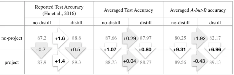
Figure 2: Comparison of the accuracy improvements reported inHu et al.(2016) and those obtained by averaging over 100 random seeds. The last two columns show the (averaged) accuracy improvements forA-but-Bstyle sentences. All models use the publicly available implementation ofHu et al.(2016) trained on phrase-level SST2 data.

bels. We observe a large amount of variation from run-to-run, which is unsurprising given the small dataset size. The inset density plot in Figure 1

shows the range of accuracies (83.47 to 87.20) along with 25, 50 and 75 percentiles.3 The figure also shows how the variance persists even after the average converges: the accuracies of 100 models trained for 20 epochs each are plotted in gray, and their average is shown in red.

We conclude that, to be reproducible, only av-eraged accuracies should be reported in this task and dataset. This mirrors the conclusion from a detailed analysis byReimers and Gurevych(2017) in the context of named entity recognition.

3.2 Performance ofHu et al.(2016)

We carry out an averaged analysis of the publicly available implementation4 of Hu et al. (2016). Our analysis reveals that the reported performance of their two mechanisms (projection and distil-lation) is in fact affected by the high variability across random seeds. Our more robust averaged analysis yields a somewhat different conclusion of their effectiveness.

InFigure 2, the first two columns show the re-ported accuracies in Hu et al. (2016) for models trained with and without distillation (correspond-ing to us(correspond-ing values π = 1andπ = 0.95t in the tth epoch, respectively). The two rows show the results for models with and without a final projec-tion into the rule-regularized space. We keep our hyper-parameters identical toHu et al.(2016).5

The baseline system (no-project, no-distill) is identical to the system ofKim(2014). All the sys-tems are trained on the phrase-level SST2 dataset

3

We use early stopping based on validation performance for all models in the density plot.

4

https://github.com/ZhitingHu/logicnn/

5_{In particular,C= 6for projection.}

with early stopping on the development set. The number inside each arrow indicates the improve-ment in accuracy by adding either the projection or the distillation component to the training al-gorithm. Note that the reported figures suggest that while both components help in improving ac-curacy, the distillation component is much more helpful than the projection component.

The next two columns, which show the re-sults of repeating the above analysis after averag-ing over 100 random seeds, contradict this claim. The averaged figures show lower overall accuracy increases, and, more importantly, they attribute these improvements almost entirely to the projec-tion component rather than the distillaprojec-tion com-ponent. To confirm this result, we repeat our av-eraged analysis restricted to only“A-but-B” sen-tences targeted by the rule (shown in the last two columns). We again observe that the effect of pro-jection is pronounced, while distillation offers lit-tle or no advantage in comparison.

4 Contextualized Word Embeddings

Traditional context-independent word embed-dings like word2vec (Mikolov et al., 2013) or GloVe (Pennington et al., 2014) are fixed vec-tors for every word in the vocabulary. In contrast, contextualized embeddings are dynamic represen-tations, dependent on the current context of the word. We hypothesize that contextualized word embeddings might inherently capture these logic rules due to increasing the effective context size for the CNN layer inKim(2014). Following the recent success of ELMo (Peters et al., 2018a) in sentiment analysis, we utilize the TensorFlow Hub implementation of ELMo6and feed these contex-tualized embeddings into our CNN model. We

fine-tune the ELMo LSTM weights along with the CNN weights on the downstream CNN task. As in

Section 3, we check performance with and without the final projection into the rule-regularized space. We present our results inTable 2.

Switching to ELMo word embeddings improves performance by 2.9 percentage points on an aver-age, corresponding to about 53 test sentences. Of these, about 32 sentences (60% of the improve-ment) correspond to A-but-B and negation style sentences, which is substantial when considering that only 24.5% of test sentences include these dis-course relations (Table 1). As further evidence that ELMo helps on these specific constructions, the non-ELMo baseline model (no-project, no-distill) gets 255 sentences wrong in the test corpus on av-erage, only 89 (34.8%) of which areA-but-Bstyle or negations.

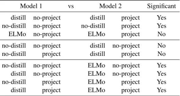
Statistical Significance: Using a two-sided Kolmogorov-Smirnov statistic (Massey Jr, 1951) withα= 0.001for the results inTable 2, we find that ELMo and projection each yield statistically significant improvements, but distillation does not. Also, with ELMo, projection is not significant. Specific comparisons have been added in the Ap-pendix, inTable A3.

KL Divergence Analysis: We observe no sig-nificant gains by projecting a trained ELMo model into anA-but-Brule-regularized space, unlike the other models. We confirm that ELMo’s predic-tions are much closer to theA-but-B rule’s man-ifold than those of the other models by computing

KL(qθ||pθ) where pθ andqθ are the original and

projected distributions: Averaged across all A-but-B sentences and 100 seeds, this gives 0.27,0.26

and 0.13 for the Kim (2014), Hu et al. (2016) with distillation and ELMo systems respectively. Intra-sentence Similarity: To understand the information captured by ELMo embeddings for A-but-B sentences, we measure the cosine simi-larity between the word vectors of every pair of words within the A-but-B sentence (Peters et al.,

2018b). We compare the intra-sentence similar-ity for fine-tunedword2vecembeddings (base-line), ELMo embeddings without fine-tuning and finally fine-tuned ELMo embeddings inFigure 3. In the fine-tuned ELMo embeddings, we notice the words within the A and within the B part of the A-but-B sentence share the same part of the vector space. This pattern is less visible in the

Model Test but butorneg

no-distill no-project 85.98 78.69 80.13

no-distill project 86.54 83.40

-distill7 no-project 86.11 79.04

-distill project 86.62 83.32

-ELMo no-project 88.89 86.51 87.24

ELMo project 88.96 87.20

-Table 2: Average performance (across 100 seeds) of ELMo on the SST2 task. We show performance onA-but-B sen-tences (“but”), negations (“neg”).

ELMo embeddings without fine-tuning and absent in theword2vecembeddings. This observation is indicative of ELMo’s ability to learn specific rules forA-but-Bsentences in sentiment classifica-tion. More intra-sentence similarity heatmaps for A-but-Bsentences are inFigure A1.

5 Crowdsourced Experiments

We conduct a crowdsourced analysis that reveals that SST2 data has significant levels of ambiguity even for human labelers. We discover that ELMo’s performance improvements over the baseline are robust across varying levels of ambiguity, whereas the advantage of Hu et al. (2016) is reversed in sentences of low ambiguity (restricting toA-but-B style sentences).

Our crowdsourced experiment was conducted on Figure Eight.8 Nineworkers scored the senti-ment of eachA-but-Band negation sentence in the test SST2 split as 0 (negative), 0.5 (neutral) or 1 (positive). (SST originally hadthree crowdwork-ers choose a sentiment rating from 1 to 25 for ev-ery phrase.) More details regarding the crowd ex-periment’s parameters have been provided in Ap-pendix A.

We average the scores across all users for each sentence. Sentences with a score in the range

(x,1]are marked as positive (wherex ∈[0.5,1)), sentences in [0,1 −x) marked as negative, and sentences in [1 − x, x] are marked as neutral. For instance, “flat , but with a revelatory perfor-mance by michelle williams” (score=0.56) is neu-tral when x = 0.6.9 We present statistics of our dataset10 in Table 3. Inter-annotator

agree-7

Trained on sentences and not phrase-level labels for a fair comparison with baseline and ELMo, unlikeSection 3.2.

8

https://www.figure-eight.com/

9_{More examples of neutral sentences have been provided} in the Appendix inTable A1, as well as a few “flipped” sen-tences receiving an average score opposite to their SST2 label (Table A2).

there are slow and repetitive parts , but it has just enough spice to keep it interesting there are slow and repetitive parts , but it has just enough spice to keep it interesting 0.1 0.0 0.1 0.2 0.3 0.4

there are slow and repetitive parts , but it has just enough spice to keep it interesting there are slow and repetitive parts , but it has just enough spice to keep it interesting 0.2 0.3 0.4 0.5

0.6 there there are slow and repetitive parts , but it has just enough spice to keep it interesting are slow and repetitive parts , but it has just enough spice to keep it interesting 0.0 0.1 0.2 0.3 0.4 0.5 0.6

Figure 3: Heat map showing the cosine similarity between pairs of word vectors within a single sentence. The left figure has fine-tunedword2vecembeddings. The middle figure contains the original ELMo embeddings without any fine-tuning. The right figure contains fine-tuned ELMo embeddings. For better visualization, the cosine similarity between identical words has been set equal to the minimum value in the heat map.

ment was computed using Fleiss’ Kappa (κ). As expected, inter-annotator agreement is higher for higher thresholds (less ambiguous sentences). Ac-cording toLandis and Koch(1977),κ∈(0.2,0.4]

corresponds to “fair agreement”, whereas κ ∈

(0.4,0.6]corresponds to “moderate agreement”. We next compute the accuracy of our model for each threshold by removing the correspond-ing neutral sentences. Higher thresholds corre-spond to sets of less ambiguous sentences.Table 3

shows that ELMo’s performance gains inTable 2

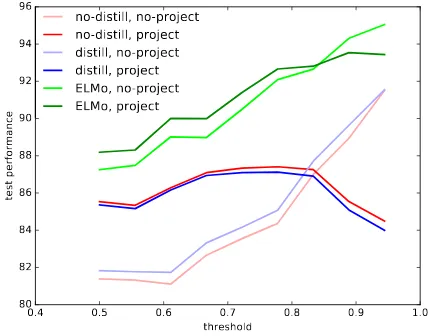
extends across all thresholds. InFigure 4we com-pare all the models on theA-but-Bsentences in this set. Across all thresholds, we notice trends similar to previous sections: 1) ELMo performs the best among all models onA-but-Bstyle sentences, and projection results in only a slight improvement; 2) models inHu et al.(2016) (with and without distil-lation) benefit considerably from projection; but 3) distillation offers little improvement (with or with-out projection). Also, as the ambiguity threshold increases, we see decreasing gains from projection on all models. In fact, beyond the 0.85 threshold, projection degrades the average performance, in-dicating that projection is useful for more ambigu-ous sentences.

6 Conclusion

We present an analysis comparing techniques for incorporating logic rules into sentiment classifi-cation systems. Our analysis included a meta-study highlighting the issue of stochasticity in performance across runs and the inherent ambi-guity in the sentiment classification task itself, which was tackled using an averaged analysis and https://github.com/martiansideofthemoon/ logic-rules-sentiment.

Threshold 0.50 0.66 0.75 0.90

Neutral Sentiment 10 70 95 234

Flipped Sentiment 15 4 2 0

Fleiss’ Kappa (κ) 0.38 0.42 0.44 0.58

no-distill, no-project 81.32 83.54 84.54 87.55

ELMo, no-project 87.56 90.00 91.31 93.14

Table 3: Number of sentences in the crowdsourced study (447 sentences) which got marked as neutral and which got the opposite of their labels in the SST2 dataset, using vari-ous thresholds. Inter-annotator agreement is computed using Fleiss’ Kappa. Average accuracies of the baseline and ELMo (over 100 seeds) on non-neutral sentences are also shown.

0.4 0.5 0.6 0.7 0.8 0.9 1.0

threshold 80 82 84 86 88 90 92 94 96 test performance no-distill, no-project no-distill, project distill, no-project distill, project ELMo, no-project ELMo, project

Figure 4: Average performance on theA-but-Bpart of the crowd-sourced dataset (210 sentences, 100 seeds)). For each threshold, only non-neutral sentences are used for evaluation.

References

Kuzman Ganchev, Jennifer Gillenwater, Ben Taskar, et al. 2010. Posterior regularization for structured latent variable models. Journal of Machine Learn-ing Research, 11(Jul):2001–2049.

Geoffrey Hinton, Oriol Vinyals, and Jeff Dean. 2015. Distilling the knowledge in a neural network. NIPS Deep Learning and Representation Learning Work-shop.

Zhiting Hu, Xuezhe Ma, Zhengzhong Liu, Eduard Hovy, and Eric Xing. 2016. Harnessing deep neural networks with logic rules. InAssociation for Com-putational Linguistics (ACL).

Mohit Iyyer, Varun Manjunatha, Jordan Boyd-Graber, and Hal Daum´e III. 2015. Deep unordered compo-sition rivals syntactic methods for text classification. InAssociation for Computational Linguistics (ACL). Yoon Kim. 2014. Convolutional neural networks for sentence classification. In Empirical Methods in Natural Language Processing (EMNLP).

J Richard Landis and Gary G Koch. 1977. The mea-surement of observer agreement for categorical data. Biometrics, pages 159–174.

Shen Li, Zhe Zhao, Tao Liu, Renfen Hu, and Xi-aoyong Du. 2017. Initializing convolutional filters with semantic features for text classification. In Empirical Methods in Natural Language Processing (EMNLP).

Frank J Massey Jr. 1951. The Kolmogorov-Smirnov test for goodness of fit. Journal of the American sta-tistical Association, 46(253):68–78.

Tomas Mikolov, Kai Chen, Greg Corrado, and Jef-frey Dean. 2013. Efficient estimation of word representations in vector space. arXiv preprint arXiv:1301.3781.

Bo Pang and Lillian Lee. 2005. Seeing stars: Ex-ploiting class relationships for sentiment categoriza-tion with respect to rating scales. InAssociation for Computational Linguistics (ACL).

Jeffrey Pennington, Richard Socher, and Christopher Manning. 2014. GloVe: Global vectors for word representation. In Empirical Methods in Natural Language Processing (EMNLP).

Matthew E. Peters, Mark Neumann, Mohit Iyyer, Matt Gardner, Christopher Clark, Kenton Lee, and Luke Zettlemoyer. 2018a. Deep contextualized word rep-resentations. In North American Association for Computational Linguistics (NAACL).

Matthew E. Peters, Mark Neumann, Wen tau Yih, and Luke Zettlemoyer. 2018b. Dissecting contextual word embeddings: Architecture and representation. InEmpirical Methods in Natural Language Process-ing (EMNLP).

Nils Reimers and Iryna Gurevych. 2017. Reporting score distributions makes a difference: Performance study of LSTM-networks for sequence tagging. In Empirical Methods in Natural Language Processing (EMNLP).

Richard Socher, Alex Perelygin, Jean Wu, Jason Chuang, Christopher D Manning, Andrew Ng, and Christopher Potts. 2013. Recursive deep models for semantic compositionality over a sentiment tree-bank. InEmpirical Methods in Natural Language Processing (EMNLP).

Kai Sheng Tai, Richard Socher, and Christopher D Manning. 2015. Improved semantic representations from tree-structured long short-term memory net-works. In Association for Computational Linguis-tics (ACL).

Appendix

A Crowdsourcing Details

Crowd workers residing in five English-speaking countries (United States, United Kingdom, New Zealand, Australia and Canada) were hired. Each crowd worker had a Level 2 or higher rating on Figure Eight, which corresponds to a “group of more experienced, higher accuracy contributors”. Each contributor had to pass a test questionnaire to be eligible to take part in the experiment. Test questions were also hidden throughout the task and untrusted contributions were removed from the final dataset. For greater quality control, an upper limit of 75 judgments per contributor was enforced.

# Judgments Average Sentence Positive Negative Neutral

1 1 7 0.50 the fight scenes are fun , but it grows tedious

3 2 4 0.56 it ’s not exactly a gourmet meal but the fare is fair ,

even coming from the drive thru

2 3 4 0.44 propelled not by characters but by caricatures

4 2 3 0.61 not everything works , but the average is higher than

in mary and most other recent comedies

Table A1: Examples of neutral sentences for a threshold of 0.66

# Judgments Average Original Sentence

Positive Negative Neutral

1 5 3 0.28 Positive

de niro and mcdormand give solid perfor-mances , but their screen time is sabotaged by the story ’s inability to create interest

6 0 3 0.83 Negative

son of the bride may be a good half hour too long but comes replete with a flattering sense of mystery and quietness

0 5 4 0.22 Positive

wasabi is slight fare indeed , with the entire project having the feel of something tossed off quickly ( like one of hubert ’s punches ) , but it should go down smoothly enough with popcorn

Table A2: Examples of flipped sentiment sentences, for a threshold of 0.66

Model 1 vs Model 2 Significant

distill no-project distill project Yes

no-distill no-project no-distill project Yes

ELMo no-project ELMo project No

no-distill no-project distill no-project No

no-distill project distill project No

no-distill no-project ELMo no-project Yes

distill no-project ELMo no-project Yes

no-distill project ELMo project Yes

distill project ELMo project Yes

all ends well , sort of , but the frenzied comic moments never click all ends well , sort of , but the frenzied comic moments never click 0.1 0.0 0.1 0.2 0.3

0.4 all ends well , sort of , but the frenzied comic moments never click all ends well , sort of , but the frenzied comic moments never click 0.1 0.2 0.3 0.4 0.5 0.6

all ends well , sort of , but the frenzied comic moments never click all ends well , sort of , but the frenzied comic moments never click 0.1 0.2 0.3 0.4 0.5

marisa tomei is good , but just a kiss is just a mess marisa tomei is good , but just a kiss is just a mess 0.1 0.0 0.1 0.2 0.3 0.4

marisa tomei is good , but just a kiss is just a mess marisa tomei is good , but just a kiss is just a mess 0.2 0.3 0.4 0.5 0.6

marisa tomei is good , but just a kiss is just a mess marisa tomei is good , but just a kiss is just a mess 0.0 0.1 0.2 0.3 0.4 0.5 0.6

the irwins emerge unscathed , but the fictional footage is unconvincing and criminally badly acted

the irwins emerge unscathed , but the fictional footage is unconvincing and criminally badly acted 0.1 0.0 0.1 0.2 0.3

the irwins emerge unscathed , but the fictional footage is unconvincing and criminally badly acted

the irwins emerge unscathed , but the fictional footage is unconvincing and criminally badly acted _0.1 0.2 0.3 0.4 0.5 0.6

the irwins emerge unscathed , but the fictional footage is unconvincing and criminally badly acted

the irwins emerge unscathed , but the fictional footage is unconvincing and criminally badly acted 0.1 0.2 0.3 0.4 0.5