Competitive generative models with structure learning for NLP
classification tasks
Kristina Toutanova Microsoft Research
Redmond, WA
Abstract
In this paper we show that generative models are competitive with and some-times superior to discriminative models, when both kinds of models are allowed to learn structures that are optimal for dis-crimination. In particular, we compare Bayesian Networks and Conditional log-linear models on two NLP tasks. We ob-serve that when the structure of the gen-erative model encodes very strong inde-pendence assumptions (a la Naive Bayes), a discriminative model is superior, but when the generative model is allowed to weaken these independence assumptions via learning a more complex structure, it can achieve very similar or better perfor-mance than a corresponding discrimina-tive model. In addition, as structure learn-ing for generative models is far more ef-ficient, they may be preferable for some tasks.
1 Introduction
Discriminative models have become the models of choice for NLP tasks, because of their ability to easily incorporate non-independent features and to more directly optimize classification accuracy. State of the art models for many NLP tasks are ei-ther fully discriminative or trained using discrim-inative reranking (Collins, 2000). These include models for part-of-speech tagging (Toutanova et al., 2003), semantic-role labeling (Punyakanok et al., 2005; Pradhan et al., 2005b) and Penn Tree-bank parsing (Charniak and Johnson, 2005).
The superiority of discriminative models has been shown on many tasks when the discrimina-tive and generadiscrimina-tive models use exactly the same model structure (Klein and Manning, 2002). How-ever, the advantage of the discriminative
mod-els can be very slight (Johnson, 2001) and for small training set sizes generative models can be better because they need fewer training sam-ples to converge to the optimal parameter setting (Ng and Jordan, 2002). Additionally, many dis-criminative models use a generative model as a base model and add discriminative features with reranking (Collins, 2000; Charniak and Johnson, 2005; Roark et al., 2004), or train discriminatively a small set of weights for features which are gener-atively estimated probabilities (Raina et al., 2004; Och and Ney, 2002). Therefore it is important to study generative models and to find ways of mak-ing them better even when they are used only as components of discriminative models.
Generative models may often perform poorly due to making strong independence assumptions about the joint distribution of features and classes. To avoid this problem, generative models for NLP tasks have often been manually designed to achieve an appropriate representation of the joint distribution, such as in the parsing models of (Collins, 1997; Charniak, 2000). This shows that when the generative models have a good model structure, they can perform quite well.
In this paper, we look differently at compar-ing generative and discriminative models. We ask the question: given the same set of input features, what is the best a generative model can do if it is allowed to learn an optimal structure for the joint distribution, and what is the best a discriminative model can do if it is also allowed to learn an op-timal structure. That is, we do not impose any in-dependence assumptions on the generative or dis-criminative models and let them learn the best rep-resentation of the data they can.
Structure learning is very efficient for genera-tive models in the form of directed graphical mod-els (Bayesian Networks (Pearl, 1988)), since the optimal parameters for such models can be esti-mated in closed form. We compare Bayesian
works with structure learning to their closely re-lated discriminative counterpart – conditional log-linear models with structure learning. Our condi-tional log-linear models can also be seen as Con-ditional Random Fields (Lafferty et al., 2001), ex-cept we do not have a structure on the labels, but want to learn a structure on the features.
We compare the two kinds of models on two NLP classification tasks – prepositional phrase at-tachment and semantic role labelling. Our re-sults show that the generative models are compet-itive with or better than the discriminative mod-els. When a small set of interpolation parame-ters for the conditional probability tables are fit discriminatively, the resulting hybrid generative-discriminative models perform better than the gen-erative only models and sometimes better than the discriminative models.
In Section 2, we describe in detail the form of the generative and discriminative models we study and our structure search methodology. In Section 3 we present the results of our empirical study.
2 Model Classes and Methodology
2.1 Generative Models
In classification tasks, given a training set of in-stances D = {[xi, yi]}, where xi are the input
features for the i-th instance, and yi is its label,
the task is to learn a classifier that predicts the la-bels of new examples. IfX is the space of inputs andY is the space of labels, a classifier is a func-tion f : X → Y. A generative model is one that models the joint probability of inputs and labels
PD(x, y) through a distribution Pθ(x, y),
depen-dent on some parameter vector θ. The classifier based on this generative model chooses the most likely label given an input according to the con-ditionalized estimated joint distribution. The pa-rametersθof the fitted distribution are usually es-timated using the maximum joint likelihood esti-mate, possibly with a prior.
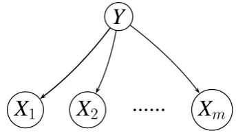
We study generative models represented as Bayesian Networks (Pearl, 1988), because their parameters can be estimated extremely fast as the maximizer of the joint likelihood is the closed form relative frequency estimate. A Bayesian Net-work is an acyclic directed graph over a set of nodes. For every variableZ, letP a(Z)denote the set of parents ofZ. The structure of the Bayesian Network encodes the following set of
indepen-Y
[image:2.595.330.502.62.159.2]X
1X
2...
Xm
Figure 1: Naive Bayes Bayesian Network
dence assumptions: every variable is conditionally independent of its non-descendants given its par-ents. For example, the structure of the Bayesian Network model in Figure 1 encodes the indepen-dence assumption that the input features are con-ditionally independent given the class label.
Let the input be represented as a vector of m
nominal features. We define Bayesian Networks over the m input variables X1, X2, . . . , Xm and
the class variableY. In all networks, we add links from the class variable Y to all input features. In this way we have generative models which estimate class-specific distributions over features
P(X|Y)and a prior over labelsP(Y). Figure 1 shows a simple Bayesian Network of this form, which is the well-known Naive Bayes model.
A specific joint distribution for a given Bayesian Network (BN) is given by a set of condi-tional probability tables (CPTs) which spec-ify the distribution over each variable given its parents P(Z|P a(Z)). The joint distribution
P(Z1, Z2, . . . , Zm)is given by:
P(Z1, Z2, . . . , Zm) = Y
i=1...m
P(Zi|P a(Zi))
The parameters of a Bayesian Network model given its graph structure are the values of the conditional probabilities P(Zi|P a(Zi)). If
the model is trained through maximizing the joint likelihood of the data, the optimal pa-rameters are the relative frequency estimates:
ˆ
P(Zi=v|P a(Zi) =~u) =
count(Zi=v,P a(Zi)=~u) count(P a(Zi)=~u) Here
vdenotes a value ofZi and~udenotes a vector of
values for the parents ofZi.
(2001). In particular, it is important to incorpo-rate lower-order information based on subsets of the conditioning information. Therefore we as-sume a structural form of the conditional proba-bility tables which implements a more sophisti-cated type of smoothing – interpolated Witten-Bell (Witten and Bell, 1991). This kind of smooth-ing has also been used in the generative parser of (Collins, 1997) and has been shown to have a rel-atively good performance for language modeling (Goodman, 2001).
To describe the form of the conditional proba-bility tables, we introduce some notation. Let Z
denote a variable in the BN and Z1, Z2, . . . , Zk
denote the set of its parents. The probabil-ityP(Z=z|Z1=z1, Z2=z2, . . . , Zk=zk)is estimated
using Witten-Bell smoothing as follows: (below the tuple of values z1, z2, . . . , zk is denoted by
z1k).
PW B(z|z1k) =λ(z1k)×Pˆ(z|z1k) + (1−λ(z1k))×PW B(z|z1k−1)
In the above equation, Pˆ is the relative fre-quency estimator. The recursion is ended by inter-polating with a uniform distribution V1
z, whereVz is the vocabulary of values for the prediction vari-able Z. We determine the interpolation back-off order by looking at the number of values of each variable. We apply the following rule: the variable with the highest number of values observed in the training set is backed off first, then the variable with the next highest number of values, and so on. Typically, the class variable will be backed-off last according to this rule.
In Witten-Bell smoothing, the values of the in-terpolation coefficients are as follows: λ(z1k) =
count(z1k)
count(z1k)+d×|z:count(z,z1k)>0|. The weight of the relative frequency estimate based on a given con-text increases if the concon-text has been seen more often in the training data and decreases if the con-text has been seen with more different values for the predicted variablez.
Looking at the form of our conditional proba-bility tables, we can see that the major parame-ters are estimated directly based on the counts of the events in the training data. In addition, there are interpolation parameters (denoted bydabove), which participate in computing the interpolation weightsλ. Thedparameters are hyper-parameters and we learn them on a development set of sam-ples. We experimented with learning a single d
parameter which is shared by all CPTs and learn-ing multipledparameters – one for every type of
conditioning context in every CPT – i.e., each CPT has as manydparameters as there are back-off lev-els.
We place some restrictions on the Bayesian Net-works learned, for closer correspondence with the discriminative models and for tractability: Every input variable node has the label node as a parent, and at most three parents per variable are allowed.
2.1.1 Structure Search Methodology
Our structure search method differs slightly from previously proposed methods in the literature (Heckerman, 1999; Pernkopf and Bilmes, 2005). The search space is defined as follows. We start with a Bayesian Network containing only the class variable. We denote by CHOSENthe set of
vari-ables already in the network and by REMAINING
the set of unplaced variables. Initially, only the class variableY is in CHOSENand all other vari-ables are in REMAINING. Starting from the cur-rent BN, the set of next candidate structures is de-fined as follows: For every unplaced variable R
in REMAINING, and for every subsetSub of size
at most two from the already placed variables in CHOSEN, consider addingRwith parentsSub∪Y to the current BN. Thus the number of candidate structures for extending a current BN is on the or-der ofm3, wheremis the number of variables.
We perform a greedy search. At each step, if the best variableBwith the best set of parentsP a(B) improves the evaluation criterion, move B from REMAININGto CHOSEN, and continue the search until there are no variables in REMAININGor the evaluation criterion can not be improved.
Notice that the optimal parameters of the con-ditional probability tables of variables already in the current BN do not change at all when a new variable is added, thus making update very ef-ficient. After the stopping criterion is met, the hyper-parameters of the resulting BN are fit on the development set. As discussed in the previ-ous subsection, we fit either a single or multiple hyper-parameters d. The fitting criterion for the generative Bayesian Networks is joint likelihood of the development set of samples with a Gaussian prior on the valueslog(d).1
Additionally, we explore fitting the hyper-parameters of the Bayesian Networks by opti-mizing the conditional likelihood of the develop-ment set of samples. In this case we call the resulting models Hybrid Bayesian Network mod-els, since they incorporate a number of discrimi-natively trained parameters. Hybrid models have been proposed before and shown to perform very competitively (Raina et al., 2004; Och and Ney, 2002). In Section 3.2 we compare generative and hybrid Bayesian Networks.
2.2 Discriminative Models
Discriminative models learn a conditional distri-bution Pθ(Y|X~) or discriminant functions that
discriminate between classes. Here we concen-trate on conditional log-linear models. A sim-ple examsim-ple of such model is logistic regression, which directly corresponds to Naive Bayes but is trained to maximize the conditional likelihood.2
To describe the form of models we study, let us introduce some notation. We represent a tuple of nominal variables (X1,X2,. . . ,Xm) as a vector of
0s and 1s in the following standard way: We map the tuple of values of nominal variables to a vector space with dimensionality the sum of possible val-ues of all variables. There is a single dimension in the vector space for every value of each input vari-able Xi. The tuple (X1,X2,. . . ,Xm) is mapped to
a vector which has 1s inm places, which are the corresponding dimensions for the values of each variableXi. We denote this mapping byΦ.
In logistic regression, the probability of a label
Y =ygiven input featuresΦ(X1, X2, . . . , Xk) =
1
Since thedparameters are positive we convert the prob-lem to unconstrained optimization over parametersγ such thatd=eγ.
2
Logistic regression additionally does not have the sum to one constraint on weights but it can be shown that this does not increase the representational power of the model.
~
xis estimated as:
P(y|~x) = Pexphw~y, ~xi y0exphw~y0, ~xi
There is a parameter vector of feature weights
~
wy for each labely. We fit the parameters of the
log-linear model by maximizing the conditional likelihood of the training set including a gaussian prior on the parameters. The prior has mean0and variance σ2. The variance is a hyper-parameter, which we optimize on a development set.
In addition to this simple logistic regression model, as for the generative models, we consider models with much richer structure. We consider more complex mappings Φ, which incorporate conjunctions of combinations of input variables. We restrict the number of variables in the com-binations to three, which directly corresponds to our limit on number of parents in the Bayesian Network structures. This is similar to consider-ing polynomial kernels of up to degree three, but is more general, because, for example, we can add only some and not all bigram conjunctions of variables. Structure search (or feature selec-tion) for log-linear models has been done before e.g. (Della Pietra et al., 1997; McCallum, 2003). We devise our structure search methodology in a way that corresponds as closely as possible to our structure search for Bayesian Networks. The ex-act hypothesis space considered is defined by the search procedure for an optimal structure we ap-ply, which we describe next.
2.2.1 Structure Search Methodology
We start with an initial empty feature set and a candidate feature set consisting of all input fea-tures: CANDIDATES={X1,X2,. . . ,Xm}. In the
course of the search, the set CANDIDATES may contain feature conjunctions in addition to the ini-tial input features. After a feature is selected from the candidates set and added to the model, the fea-ture is removed from CANDIDATES and all con-junctions of that feature with all input features are added to CANDIDATES. For example, if a fea-ture conjunctionhXi1,Xi2,. . .,Xiniis selected, all of its expansions of the formhXi1,Xi2,. . .,Xin,Xii, where Xi is not in the conjunction already, are
added to CANDIDATES.
CANDIDATESas described above. The evaluation
criterion for selecting features is classification ac-curacy on a development set of samples, as for the Bayesian Network structure search.
At each step, we evaluate all candidate fea-tures. This is computationally expensive, because it requires iterative re-estimation. In addition to estimating weights for the new features, we re-estimate the old parameters, since their optimal values change. We did not preform search for the hyper-parameterσwhen evaluating models. We fit
σ by optimizing the development set accuracy af-ter a model was selected. Note that our feature se-lection algorithm adds an input variable or a vari-able conjunction with all of its possible values in a single step of the search. Therefore we are adding hundreds or thousands of binary features at each step, as opposed to only one as in (Della Pietra et al., 1997). This is why we can afford to per-form complete re-estimation of the parameters of the model at each step.
3 Experiments
3.1 Problems and Datasets
We study two classification problems – preposi-tional phrase (PP) attachment, and semantic role labeling.
Following most of the literature on preposi-tional phrase attachment (e.g., (Hindle and Rooth, 1993; Collins and Brooks, 1995; Vanschoen-winkel and Manderick, 2003)), we focus on the most common configuration that leads to ambi-guities: V NP PP. Here, we are given a verb phrase with a following noun phrase and a prepo-sitional phrase. The goal is to determine if the PP should be attached to the verb or to the ob-ject noun phrase. For example, in the sentence:
Never [hang]V [a painting]NP [with a peg]PP, the prepositional phrase with a peg can either modify the verb hang or the object noun phrase a painting. Here, clearly, with a peg modifies the verb hang.
We follow the common practice in representing the problem using only the head words of these constituents and of the NP inside the PP. Thus the example sentence is represented as the following quadruple: [v:hang n1:painting p:with n2:peg]. Thus for the PP attachment task we have binary labelsAtt, and four input variables –v, n1, p, n2.
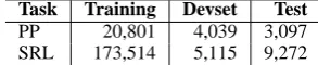
We work with the standard dataset previously used for this task by other researchers
(Ratna-Task Training Devset Test
PP 20,801 4,039 3,097
[image:5.595.341.488.63.93.2]SRL 173,514 5,115 9,272
Table 1: Data sizes for the PP attachment and SRL tasks.
parkhi et al., 1994; Collins and Brooks, 1995). It is extracted from the the Penn Treebank Wall Street Journal data (Ratnaparkhi et al., 1994). Table 1 shows summary statistics for the dataset.
The second task we concentrate on is semantic role labeling in the context of PropBank (Palmer et al., 2005). The PropBank corpus annotates phrases which fill semantic roles for verbs on top of Penn Treebank parse trees. The annotated roles specify agent, patient, direction, etc. The labels for semantic roles are grouped into two groups,
core argument labels and modifier argument
la-bels, which correspond approximately to the tradi-tional distinction between arguments and adjuncts.
There has been plenty of work on machine learning models for semantic role labeling, start-ing with the work of Gildea and Jurafsky (2002), and including CoNLL shared tasks (Carreras and M`arquez, 2005). The most successful formulation has been as learning to classify nodes in a syn-tactic parse tree. The possible labels are NONE, meaning that the corresponding phrase has no se-mantic role and the set of core and modifier la-bels. We concentrate on the subproblem of
clas-sification for core argument nodes. The problem
is, given that a node has a core argument label, de-cide what the correct label is. Other researchers have also looked at this subproblem (Gildea and Jurafsky, 2002; Toutanova et al., 2005; Pradhan et al., 2005a; Xue and Palmer, 2004).
Many features have been proposed for build-ing models for semantic role labelbuild-ing. Initially, 7 features were proposed by (Gildea and Juraf-sky, 2002), and all following research has used these features and some additional ones. These are the features we use as well. Table 2 lists the features. State-of-the-art models for the subprob-lem of classification of core arguments addition-ally use other features of individual nodes (Xue and Palmer, 2004; Pradhan et al., 2005a), as well as global features including the labels of other nodes in parse tree. Nevertheless it is interesting to see how well we can do with these 7 features only.
Feature Types (Gildea and Jurafsky, 2002) PHRASETYPE: Syntactic Category of node PREDICATELEMMA: Stemmed Verb PATH: Path from node to predicate POSITION: Before or after predicate? VOICE: Active or passive relative to predicate HEADWORD OFPHRASE
SUB-CAT: CFG expansion of predicate’s parent
Table 2: Features for Semantic Role Labeling.
test sets from the February 2004 version of Prop-bank. The training set consists of sections 2 to 21, the development set is from section 24, and the test set is from section 23. The number of samples is listed in Table 1. As we can see, the training set size is much larger compared to the PP attachment training set.
3.2 Results
In line with previous work (Ng and Jordan, 2002; Klein and Manning, 2002), we first compare Naive Bayes and Logistic regression on the two NLP tasks. This lets us see how they compare when the generative model is making strong independence assumptions and when the two kinds of models have the same structure. Then we compare the generative and discriminative models with learned richer structures.
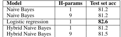
Table 3 shows the Naive Bayes/Logistic gression results for PP attachment. We list re-sults for several conditions of training the Naive Bayes classifier, depending on whether it is trained as strictly generative or as a hybrid model, and whether a single or multiple hyper-parameters d
are trained. In the table, we see results for gen-erative Naive Bayes, where the dparameters are trained to maximize the joint likelihood of the de-velopment set, and for Hybrid Naive Bayes, where the hyper-parameters are trained to optimize the conditional likelihood. The column H-Params (for hyper-parameters) indicates whether a single or multipledparameters are learned.
Logistic regression is more fairly comparable to Naive Bayes trained using a single parameter, because it also uses a single hyper-parameter σ trained on a development set. How-ever, for the generative model it is very easy to train multiple weights dsince the likelihood of a development set is differentiable with respect to the parameters. For logistic regression, we may want to choose different variances for the differ-ent types of features but the search would be
pro-Model H-params Test set acc
Naive Bayes 1 81.2
Naive Bayes 9 81.2
Logistic regression 1 82.6
Hybrid Naive Bayes 1 81.2
[image:6.595.316.514.62.123.2]Hybrid Naive Bayes 9 81.5
Table 3: Naive Bayes and Logistic regression PP attachment results.
hibitively expensive. Thus we think it is also fair to fit multiple interpolation weights for the gener-ative model and we show these results as well.
As we can see from the table, logistic regression outperforms both Naive Bayes and Hybrid Naive Bayes. The performance of Hybrid Naive Bayes with multiple interpolation weights improves the accuracy, but performance is still better for logis-tic regression. This suggests that the strong in-dependence assumptions are hurting the classifier. According to McNemar’s test, logistic regression is statistically significantly better than the Naive Bayes models and than Hybrid Naive Bayes with a single interpolation weight (p <0.025), but is not significantly better than Hybrid Naive Bayes with multiple interpolation parameters at level 0.05.
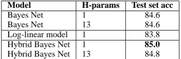
However, when both the generative and dis-criminative models are allowed to learn optimal structures, the generative model outperforms the discriminative model. As seen from Table 4, the Bayesian Network with a single interpolation weight achieves an accuracy of 84.6%, whereas the discriminative model performs at83.8%. The hybrid model with a single interpolation weight does even better, achieving85.0%accuracy. For comparison, the model of Collins & Brooks has accuracy of 84.15% on this test set, and the high-est result obtained through a discriminative model with this feature set is84.8%, using SVMs and a polynomial kernel with multiple hyper-parameters (Vanschoenwinkel and Manderick, 2003). The Hybrid Bayes Nets are statistically significantly better than the Log-linear model (p < 0.05), and the Bayes Nets are not significantly better than the Log-linear model. All models from Table 4 are significantly better than all models in Table 3.
Model H-params Test set acc
Bayes Net 1 84.6
Bayes Net 13 84.6
Log-linear model 1 83.8
Hybrid Bayes Net 1 85.0
[image:7.595.88.275.62.123.2]Hybrid Bayes Net 13 84.8
Table 4: Bayesian Network and Conditional log-linear model PP attachment results.
Model H-params Test set acc
Naive Bayes 1 83.3
Naive Bayes 15 85.2
Logistic regression 1 91.1
Hybrid Naive Bayes 1 84.1
[image:7.595.324.509.62.122.2]Hybrid Naive Bayes 15 86.5
Table 5: Naive Bayes and Logistic regression SRL classificaion results.
strong, and since many of the features are not sparse lexical features and training data for them is sufficient, the Naive Bayes model has no ad-vantage over the discriminative logistic regression model. The Hybrid Naive Bayes model with mul-tiple interpolation weights does better than Naive Bayes, performing at 86.5%. All differences be-tween the classifiers in Table 5 are statistically sig-nificant at level 0.01. Compared to the PP attach-ment task, here we are getting more benefit from multiple hyper-parameters, perhaps due to the di-versity of the features for SRL: In SRL, we use both sparse lexical features and non-sparse syntac-tic ones, whereas all features for PP attachment are lexical.
From Table 6 we can see that when we com-pare general Bayesian Network structures to gen-eral log-linear models, the performance gap be-tween the generative and discriminative models is much smaller. The Bayesian Network with a single interpolation weightdhas 93.5% accuracy and the log-linear model has 93.9% accuracy. The hybrid model with multiple interpolation weights performs at 93.7%. All models in Table 6 are in a statistical tie according to McNemar’s test, and thus the log-linear model is not significantly bet-ter than the Bayes Net models. We can see that the generative model was able to learn a structure with a set of independence assumptions which are not as strong as the ones the Naive Bayes model makes, thus resulting in a model with performance competitive with the discriminative model.
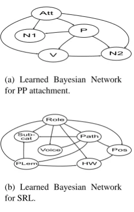
Figures 2(a) and 2(b) show the Bayesian Net-works learned for PP Attachment and Semantic Role Labeling. Table 7 shows the conjunctions
Model H-params Test set acc
Bayes Net 1 93.5
Bayes Net 20 93.6
Log-linear model 1 93.9
Hybrid Bayes Net 1 93.5
Hybrid Bayes Net 20 93.7
Table 6: Bayesian Network and Conditional log-linear model SRL classification results.
PP Attachment Model hPi,hP,Vi,hP,N1i,hP,N2i hN1i,hVi,hP,N1,N2i SRL Model
[image:7.595.323.511.165.253.2]hPATHi,hPATH,PLEMMAi,hSUB-CATi,hPLEMMAi hHW,PLEMMAi,hPATH,PLEMMA,VOICEi ,hHW,PLEMMA,PTYPEi,hSUB-CAT,PLEMMAi hSUB-CAT,PLEMMA,POSi,hHWi
Table 7: Log-linear models learned for PP attach-ment and SRL.
learned by the Log-linear models for PP attach-ment and SRL.
We should note that it is much faster to do structure search for the generative Bayesian Net-work model, as compared to structure search for the log-linear model. In our implementation, we did not do any computation reuse between succes-sive steps of structure search for the Bayesian Net-work or log-linear models. Structure search took 2 hours for the Bayesian Network and 24 hours for the log-linear model.
To put our results in the context of previous work, other results on core arguments using the same input features have been reported, the best being 91.4% for an SVM with a degree 2 poly-nomial kernel (Pradhan et al., 2005a).3 The highest reported result for independent classifica-tion of core arguments is 96.0% for a log-linear model using more than 20 additional basic features (Toutanova et al., 2005). Therefore our resulting models with 93.5% and 93.9% accuracy compare favorably to the SVM model with polynomial ker-nel and show the importance of structure learning.
4 Comparison to Related Work
Previous work has compared generative and dis-criminative models having the same structure, such as the Naive Bayes and Logistic regression models (Ng and Jordan, 2002; Klein and Man-ning, 2002) and other models (Klein and ManMan-ning, 2002; Johnson, 2001).
3This result is on an older version of Propbank from July
[image:7.595.84.280.169.232.2]Att
P N1
N2 V
(a) Learned Bayesian Network for PP attachment.
Role
Sub-cat Path
Voice
PLem HW
Pos
[image:8.595.117.253.66.280.2](b) Learned Bayesian Network for SRL.
Figure 2: Learned Bayesian Network structures for PP attachment and SRL.
Bayesian Networks with special structure of the CPTs – e.g. decision trees, have been previously studied in e.g. (Friedman and Goldszmidt, 1996), but not for NLP tasks and not in comparison to dis-criminative models. Studies comparing generative and discriminative models with structure learn-ing have been previously performed ((Pernkopf and Bilmes, 2005) and (Grossman and Domingos, 2004)) for other, non-NLP domains. There are several important algorithmic differences between our work and that of (Pernkopf and Bilmes, 2005; Grossman and Domingos, 2004). We detail the differences here and perform an empirical evalua-tion of the impact of some of these differences.
Form of the generative models. The
genera-tive models studied in that previous work do not employ any special form of the conditional prob-ability tables. Pernkopf and Bilmes (2005) use a simple smoothing method: fixing the probability of every event that has a zero relative frequency estimate to a small fixed . Thus the model does not take into account information from lower or-der distributions and has no hyper-parameters that are being fit. Grossman and Domingos (2004) do not employ a special form of the CPTs either and do not mention any kind of smoothing used in the generative model learning.
Form of the discriminative models. The works (Pernkopf and Bilmes, 2005; Grossman and Domingos, 2004) study Bayesian Networks whose parameters are trained discriminatively (by
maximizing conditional likelihood), as represen-tatives of discriminative models. We study more general log-linear models, equivalent to Markov Random Fields. Our models are more general in that their parameters do not need to be inter-pretable as probabilities (sum to 1 and between 0 and 1), and the structures do not need to corre-spond to Bayes Net structures. For discriminative classifiers, it is not important that their compo-nent parameters be interpretable as probabilities; thus this restriction is probably unnecessary. Like for the generative models, another major differ-ence is in the smoothing algorithms. We smooth the models both by fitting a gaussian prior hyper-parameter and by incorporating features of subsets of cliques. Smoothing in (Pernkopf and Bilmes, 2005) is done by substituting zero-valued param-eters with a small fixed. Grossman and Domin-gos (2004) employ early stopping using held-out data which can achieve similar effects to smooth-ing with a gaussian prior.
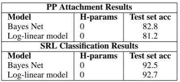
To evaluate the importance of the differences between our algorithm and the ones presented in these works, and to evaluate the importance of fit-ting hyper-parameters for smoothing, we imple-mented a modified version of our structure search. The modifications were as follows. For Bayes Net structure learning: (i) no Witten-Bell smooth-ing is employed in the CPTs, and (ii) no backoffs to lower-order distributions are considered. The only smoothing remaining in the CPTs is an inter-polation with a uniform distribution with a fixed weight of α = .1. For discriminative log-linear model structure learning: (i) the gaussian prior was fixed to be very weak, serving only to keep the weights away from infinity (σ = 100) and (ii) the conjunction selection was restricted to correspond to a Bayes Net structure with no features for sub-sets of feature conjunctions. Thus the only differ-ence between the class of our modified discrimina-tive log-linear models and the class of models con-sidered in (Pernkopf and Bilmes, 2005; Grossman and Domingos, 2004) is that we do not restrict the parameters to be interpretable as probabilities.
PP Attachment Results
Model H-params Test set acc
Bayes Net 0 82.8
Log-linear model 0 81.2
SRL Classification Results
Model H-params Test set acc
Bayes Net 0 92.5
[image:9.595.89.275.60.145.2]Log-linear model 0 92.7
Table 8: Bayesian Network and Conditional log-linear model: PP & SRL classification results us-ing minimal smoothus-ing and no backoff to lower order distributions.
In summary, our results showed that by learning the structure for generative models, we can obtain models which are competitive with or better than corresponding discriminative models. We also showed the importance of employing sophisti-cated smoothing techniques in structure search al-gorithms for natural language classification tasks.
References
Xavier Carreras and Lu´ıs M`arquez. 2005. Introduction to the CoNLL-2005 shared task: Semantic role labeling. In
Proceedings of CoNLL.
Eugene Charniak and Mark Johnson. 2005. Coarse-to-fine n-best parsing and MaxEnt discriminative reranking. In
Proceedings of ACL.
Eugene Charniak. 2000. A maximum-entropy-inspired parser. In Proceedings of NAACL, pages 132–139. Michael Collins and James Brooks. 1995. Prepositional
at-tachment through a backed-off model. In Proceedings of
the Third Workshop on Very Large Corpora, pages 27–38.
Michael Collins. 1997. Three generative, lexicalised models for statistical parsing. In Proceedings of ACL, pages 16 – 23.
Michael Collins. 2000. Discriminative reranking for natural language parsing. In Proceedings of ICML, pages 175– 182.
Stephen Della Pietra, Vincent J. Della Pietra, and John D. Lafferty. 1997. Inducing features of random fields. IEEE
Transactions on Pattern Analysis and Machine Intelli-gence, 19(4):380–393.
Nir Friedman and Moises Goldszmidt. 1996. Learning Bayesian networks with local structure. In Proceeding of
UAI, pages 252–262.
Daniel Gildea and Daniel Jurafsky. 2002. Automatic labeling of semantic roles. Computational Linguistics, 28(3):245– 288.
Joshua T. Goodman. 2001. A bit of progress in language modeling. In MSR Technical Report MSR-TR-2001-72. Daniel Grossman and Pedro Domingos. 2004. Learning
bayesian network classifiers by maximizing conditional likelihood. In Proceedings of ICML, pages 361—368. David Heckerman. 1999. A tutorial on learning with bayesian
networks. In Learning in Graphical Models. MIT Press. Donald Hindle and Mats Rooth. 1993. Structural
ambi-guity and lexical relations. Computational Linguistics,
19(1):103–120.
Mark Johnson. 2001. Joint and conditional estimation of tagging and parsing models. In Proceedings of ACL. Dan Klein and Christopher Manning. 2002. Conditional
structure versus conditional estimation in NLP models. In
Proceedings of EMNLP.
John Lafferty, Andrew McCallum, and Fernando Pereira. 2001. Conditional random fields: Probabilistic models for segmenting and labeling sequence data. In Proc. 18th
In-ternational Conf. on Machine Learning, pages 282–289.
Morgan Kaufmann, San Francisco, CA.
Andrew McCallum. 2003. Efficiently inducing features of conditional random fields. In Proceedings of UAI. Andrew Ng and Michael Jordan. 2002. On discriminative vs.
generative classifiers: A comparison of logistic regression and Naive Bayes. In NIPS 14.
Franz Josef Och and Hermann Ney. 2002. Discriminative training and maximum entropy models for statistical ma-chine translation. In Proceedings of ACL, pages 295–302. Martha Palmer, Dan Gildea, and Paul Kingsbury. 2005. The proposition bank: An annotated corpus of semantic roles.
Computational Linguistics.
Judea Pearl. 1988. Probabilistic reasoning in intelligent systems: Networks of plausible inference. Morgan
Kauf-mann.
Franz Pernkopf and Jeff Bilmes. 2005. Discriminative versus generative parameter and structure learning of bayesian network classifiers. In Proceedings of ICML.
Sameer Pradhan, Kadri Hacioglu, Valerie Krugler, Wayne Ward, James Martin, and Dan Jurafsky. 2005a. Support vector learning for semantic argument classification.
Ma-chine Learning Journal.
Sameer Pradhan, Wayne Ward, Kadri Hacioglu, James Mar-tin, and Daniel Jurafsky. 2005b. Semantic role labeling using different syntactic views. In Proceedings of ACL. Vasin Punyakanok, Dan Roth, and Wen tau Yih. 2005. The
necessity of syntactic parsing for semantic role labeling. In Proceedings of IJCAI.
Rajat Raina, Yirong Shen, Andrew Y. Ng, and Andrew McCallum. 2004. Classification with hybrid genera-tive/discriminative models. In Sebastian Thrun, Lawrence Saul, and Bernhard Sch ¨olkopf, editors, Advances in
Neu-ral Information Processing Systems 16. MIT Press,
Cam-bridge, MA.
Adwait Ratnaparkhi, Jeff Reynar, and Salim Roukos. 1994. A maximum entropy model for prepositional phrase attach-ment. In Workshop on Human Language Technology. Brian Roark, Murat Saraclar, Michael Collins, and Mark
Johnson. 2004. Discriminative language modeling with conditional random fields and the perceptron algorithm. In Proceedings of ACL.
Kristina Toutanova, Dan Klein, and Christopher D. Manning. 2003. Feature-rich part-of-speech tagging with a cyclic dependency network. In Proceedings of HLT-NAACL. Kristina Toutanova, Aria Haghighi, and Christopher D.
Man-ning. 2005. Joint learning improves semantic role label-ing. In Proceedings of ACL.
Bram Vanschoenwinkel and Bernard Manderick. 2003. A weighted polynomial information gain kernel for resolv-ing prepositional phrase attachment ambiguities with sup-port vector machines. In IJCAI.
Ian H. Witten and Timothy C. Bell. 1991. The zero-frequency problem: Estimating the probabilities of novel events in adaptive text compression. IEEE Transactions on
Infor-mation Theory, 37,4:1085–1094.