Modeling Annotators:
A Generative Approach to Learning from Annotator Rationales
∗Omar F. Zaidan and Jason Eisner
Dept. of Computer Science, Johns Hopkins University Baltimore, MD 21218, USA
{ozaidan,jason}@cs.jhu.edu
Abstract
A human annotator can provide hints to a machine learner by highlighting contextual “rationales” for each of his or her annotations (Zaidan et al., 2007). How can one exploit this side information to better learn the desired parameters θ? We present a generative model of how a given annotator, knowing the true θ, stochastically chooses rationales. Thus, observing the rationales helps us infer the true θ. We collect substring rationales for a sentiment classification task (Pang and Lee, 2004) and use them to obtain significant accuracy improvements for each annotator. Our new generative approach exploits the rationales more effectively than our previous “masking SVM” approach. It is also more principled, and could be adapted to help learn other kinds of probabilistic classi-fiers for quite different tasks.
1 Background
Many recent papers aim to reduce the amount of an-notated data needed to train the parameters of a sta-tistical model. Well-known paradigms include ac-tive learning, semi-supervised learning, and either domain adaptation or cross-lingual transfer from ex-isting annotated data.
A rather different paradigm is to change the ac-tualtask that is given to annotators, giving them a greater hand in shaping the learned classifier. Af-ter all, human annotators themselves are more than just black-box classifiers to be run on training data. They possess some introspective knowledge about their own classification procedure. The hope is to mine this knowledge rapidly via appropriate ques-tions and use it to help train a machine classifier. Howto do this, however, is still being explored.
1.1 Hand-crafted rules
An obvious option is to have the annotators directly express their knowledge by hand-crafting rules. This
∗
This work was supported by National Science Foundation grant No. 0347822 and the JHU WSE/APL Partnership Fund. Special thanks to Christine Piatko for many useful discussions.
approach remains “data-driven” if the annotators re-peatedly refine their system against a corpus of la-beled or unlala-beled examples. This achieves high performance in some domains, such as NP chunk-ing (Brill and Ngai, 1999), but requires more analyt-ical skill from the annotators. One empiranalyt-ical study (Ngai and Yarowsky, 2000) found that it also re-quired more annotation time than active learning.
1.2 Feature selection by humans
More recent work has focused on statistical classi-fiers. Training such classifiers faces the “credit as-signment problem.” Given a training examplexwith many features, which features are responsible for its annotated classy? It may take many training exam-ples to distinguish useful vs. irrelevant features.1
To reduce the number of training examples needed, one can ask annotators to examine or pro-pose some candidate features. This is possible even for the very large feature sets that are typically used in NLP. In document classification, Raghavan et al. (2006) show that feature selection by an oracle could be helpful, and that humans are both rapid and rea-sonably good at distinguishing highly usefuln-gram features from randomly chosen ones, even when viewing thesen-grams out of context.
Druck et al. (2008) show annotators some features
f from a fixed feature set, and ask them to choose a class labelysuch thatp(y|f)is as high as possible. Haghighi and Klein (2006) do the reverse: for each class labely, they ask the annotators to propose a few “prototypical” featuresf such thatp(y|f)is as high as possible.
1.3 Feature selection in context
The above methods consider features out of context. An annotator might have an easier time examining
1
Most NLP systems use thousands or millions of features, because it is helpful to include lexical features over a large vo-cabulary, often conjoined with lexical or non-lexical context.
featuresin contextto recognize whether they appear relevant. This is particularly true for features that are only modestly or only sometimes helpful, which may be abundant in NLP tasks.
Thus, Raghavan et al. (2006) propose an active learning method in which, while classifying a train-ing document, the annotator also identifies some fea-tures ofthatdocument as particularly relevant. E.g., the annotator might highlight particular unigrams as he or she reads the document. In their proposal, a feature that is highlighted in any document is as-sumed to be globally more relevant. Its dimension in feature space is scaled by a factor of 10 so that this feature has more influence on distances or inner products, and hence on the learned classifier.
1.4 Concerns about marking features
Despite the success of the above work, we have several concerns about asking annotators to identify globally relevant features.
First, a feature in isolation really does not have a well-defined worth. A feature may be useful only in conjunction with other features,2 or be useful only to the extent that other correlated features are not selected to do the same work.
Second, it is not clear how an annotator would easily view and highlight features in context, ex-cept for the simplest feature sets. In the phrase
Apple shares up 3%, there may be several fea-tures that fire on the substring Apple—responding to the string Apple, its case-invariant form apple, its lemmaapple-(which would also respond to ap-ples), its context-dependent senseApple2, its part
of speechnoun, etc. How does the annotator indi-cate which of these features are relevant?
Third, annotating features is only appropriate when the feature set can be easily understood by a human. This is not always the case. It would be hard for annotators to read, write, or evaluate a descrip-tion of a complex syntactic configuradescrip-tion in NLP or a convolution filter in machine vision.
Fourth, traditional annotation efforts usually try to remain agnostic about the machine learning methods
2
For example, a linear classifier can learn that most training examples satisfyA→Bby settingθA=−5andθA∧B = +5,
but this solution requires selecting bothAandA∧Bas features. More simply, a polynomial kernel can consider the conjunction
A∧Bonly if bothAandBare selected as features.
and features to be used. The project’s cost is justi-fied by saying that the annotations will be reused by many researchers (perhaps in a “shared task”), who are free to compete on how they tackle the learning problem. Unfortunately, feature annotation commits to a particular feature set at annotation time. Subse-quent research cannot easily adjust the definition of the features, or obtain annotation of new features.
2 Annotating Rationales
To solve these problems, we propose that annotators should not select features but rather mark relevant portions of the example. In earlier work (Zaidan et al., 2007), we called these markings “rationales.”
For example, when classifying a movie review as positive or negative, the annotator would also high-light phrases that supported that judgment. Figure 1 shows two such rationales.
A multi-annotator timing study (Zaidan et al., 2007) found that highlighting rationale phrases while reading movie reviews only doubled annota-tion time, although annotators marked 5–11 ratio-nale substrings in addition to the simple binary class. The benefit justified the extra time. Furthermore, much of the benefit could have been obtained by giv-ing rationales for only a fraction of the reviews.
In the visual domain, when classifying an im-age as containing a zoo, the annotator might circle some animals or cages and the sign reading “Zoo.” The Peekaboomgame(von Ahn et al., 2006) was in fact built to elicit such approximate yet relevant re-gions of images. Further scenarios were discussed in (Zaidan et al., 2007): rationale annotation for named entities, linguistic relations, or handwritten digits.
Annotating rationales does not require the anno-tator to think about the feature space, nor even to know anything about it. Arguably this makes an-notation easier and more flexible. It also preserves the reusability of the annotated data. Anyone is free to reuse our collected rationales (section 4) to aid in learning a classifier with richer features, or a dif-ferent kind of classifier altogether, using either our procedures or novel procedures.
3 Modeling Rationale Annotations
We wish to learn the parameters θ of some classi-fier. How can the annotator’s rationales help us to do this without many training examples? We will have to exploit a presumed relationship between the rationales and the optimal value ofθ(i.e., the value that we would learn on an infinite training set).
This paper exploits an explicit, parametric model of that relationship. The model’s parametersφare intended to capture what that annotator is doing when he or she marks rationales. Most importantly, they capture how he or she is influenced by the true
θ. Given this, our learning method will prefer values ofθthat would adequately explain the rationales (as well as the training classifications).
3.1 A generative approach
For concreteness, we will assume that the task is document classification. Our training data consists ofntriples{(x1, y1, r1), ...,(xn, yn, rn)}), wherexi
is a document,yi is its annotated class, andri is its
rationale markup. At test time we will have to pre-dictyn+1fromxn+1, without anyrn+1.
We propose to jointly choose parameter vectorsθ
andφto maximize the following regularized condi-tional likelihood:3
n Y
i=1
p(yi, ri|xi, θ, φ)·pprior(θ, φ) (1)
def
= n Y
i=1
pθ(yi|xi)·pφ(ri |xi, yi, θ)·pprior(θ, φ)
Here we are trying to model all the annotations, both
yi andri. The first factor predictsyi using an
ordi-nary probabilistic classifierpθ, while the novel
sec-ond factor predictsri using a modelpφ of how
an-notators generate the rationale annotations.
The crucial point is that the second factor depends onθ(sinceri is supposed to reflect the relation
be-tweenxi andyi that is modeled by θ). As a result,
the learner has an incentive to modify θ in a way that increases the second factor, even if this some-what decreases the first factor on training data.4
3
It would be preferable to integrate outφ(and evenθ), but more difficult.
4Interestingly, even examples where the annotation y
i is
wrong or unhelpful can provide useful information aboutθvia the pair(yi, ri). Two annotators marking the same movie
re-view might disagree on whether it is overall a positive or
nega-After training, one should simply use the first fac-torpθ(y |x)to classify test documentsx. The
sec-ond factor is irrelevant for test documents, since they have not been annotated with rationalesr.
The second factor may likewise be omitted for any training documents ithat have not been annotated with rationales, as there is nori to predict in those
cases. In the extreme case where no documents are annotated with rationales, equation (1) reduces to the standard training procedure.
3.2 Noisy channel design of rationale models
Like ordinary class annotations, rationale annota-tions present us with a “credit assignment problem,” albeit a smaller one that is limited to features that fire “in the vicinity” of the rationaler. Some of these
θ-features were likely responsible for the classifica-tionyand hence triggered the rationale. Other such
θ-features were just innocent bystanders.
Thus, the interesting part of our model is pφ(r |
x, y, θ), which models the rationale annotation pro-cess.The rationalesrreflectθ, but in noisy ways.
Taking this noisy channel idea seriously, pφ(r |
x, y, θ)should consider two questions when assess-ing whether r is a plausible set of rationales given
θ. First, it needs a “language model” of rationales: does r consist of rationales that are well-formed a priori, i.e., beforeθis considered? Second, it needs a “channel model”: doesr faithfully signal the fea-tures ofθthat strongly support classifyingxasy?
If a feature contributes heavily to the classification of documentx as classy, then the channel model should tell us whichpartsof documentxtend to be highlighted as a result.
The channel model must know about the partic-ular kinds of features that are extracted by f and scored byθ. Suppose the featurenot . . . gripping,5 with weightθh, is predictive of the annotated classy.
This raises the probabilities of the annotator’s high-lighting each of various words, or combinations of words, in a phrase likenot the most gripping ban-quet on film. The channel model parameters inφ
tive review—but the second factor still allows learning positive features from the first annotator’s positive rationales, and nega-tive features from the second annotator’s neganega-tive rationales.
5
should specify howmucheach of these probabilities is raised, based on the magnitude of θh ∈ R, the
class y, and the fact that the feature is an instance of the template<Neg>. . .<Adjective>. (Thus,φ
has no parameters specific to the word gripping; it is a low-dimensional vector that only describes the annotator’s general style in translatingθintor.)
Thelanguage model, however, is independent of the feature setθ. It models what rationales tend to look like in the input domain—e.g., documents or images. In the document case, φ should describe: How frequent and how long are typical rationales? Do their edges tend to align with punctuation or ma-jor syntactic boundaries inx? Are they rarer in the middle of a document, or in certain documents?6
Thanks to the language model, we do not need to posit highθfeatures to explain every word in a ratio-nale. The language model can “explain away” some words as having been highlighted only because this annotator prefers not to end a rationale in mid-phrase, or prefers to sweep up close-together fea-tures with a single long rationale rather than many short ones. Similarly, the language model can help explain why some words, though important, might nothave been included in any rationale ofr.
If there are multiple annotators, one can learn dif-ferent φ parameters for each annotator, reflecting their different annotation styles.7 We found this to be useful (section 8.2).
We remark that our generative modeling approach (equation (1)) would also apply ifr were not ratio-nale markup, but some other kind of so-called “side information,” such as the feature annotations dis-cussed in section 1. For example, Raghavan et al. (2006) assume that if feature h is relevant—a
bi-6Our current experiments do not model this last point. How-ever, we imagine that if the document only has a fewθ-features that support the classification, the annotator will probably mark most of them, whereas if such features are abundant, the anno-tator may lazily mark only a few of the strongest ones. A simple approach would equipφwith a different “bias” or “threshold” parameterφx for each rationale training documentx, to
mod-ulate thea prioriprobability of marking a rationale inx. By fitting this bias parameter, we deduce how lazy the annotator was (for whatever reason) on documentx. If desired, a prior on φx could consider whetherxhas many strongθ-features,
whether the annotator has recently had a coffee break, etc. 7
Given insufficient rationale data to recover some annota-tor’sφwell, one could smooth using data from other annotators. But in our situation,φhad relatively few parameters to learn.
nary distinction—iff it was selected in at least one document. But it might be more informative to ob-serve thath was selected in 3 of the 10 documents where it appeared, and to predict this via a model
pφ(3 of 10|θh), whereφdescribes (e.g.) how to
de-rive a binomial parameter nonlinearly fromθh. This
approach would nothow oftenhwas marked and in-ferhow relevantis featureh (i.e., inferθh). In this
case,pφis a simple channel that transforms relevant
features into direct indicators of the feature. Our side information merely requires a more complex transformation—from relevant features into well-formed rationales, modulated by documents.
4 Experimental Data: Movie Reviews
In Zaidan et al. (2007), we introduced the “Movie Review Polarity Dataset Enriched with Annotator Rationales.”8 It is based on the dataset of Pang and
Lee (2004),9 which consists of 1000 positive and 1000 negative movie reviews, tokenized and divided into 10 folds (F0–F9). All our experiments useF9
as their final blind test set.
The enriched dataset adds rationale annotations produced by an annotator A0, who annotated folds
F0–F8of the movie review set with rationales (in the
form of textual substrings) that supported the gold-standard classifications. We will use A0’s data to determine the improvement of our method over a (log-linear) baseline model without rationales. We also use A0 to compare against the “masking SVM” method and SVM baseline of Zaidan et al. (2007).
Sinceφcan be tuned to a particular annotator, we would also like to know how well this works with data from annotators other than A0. We randomly selected 100 reviews (50 positive and 50 negative) and collected both class and rationale annotation data from each of six new annotators A3–A8,10 fol-lowing the same procedures as (Zaidan et al., 2007). We report results using only data from A3–A5, since we used the data from A6–A8 as development data in the early stages of our work.
We use this new rationale-enriched dataset8to de-termine if our method works well across annotators. We will only be able to carry out that comparison
8
Available at http://cs.jhu.edu/∼ozaidan/rationales. 9Polarity dataset version 2.0.
Figure 1: Rationales as sequence an-notation: the annotator highlighted two textual segments as rationales for a positive class. Highlighted words in
~
xare taggedIin~r, and other words are tagged O. The figure also shows someφ-features. For instance,gO(,)-I is a count ofO-Itransitions that occur with a comma as the left word. Notice also that grelis the sum of the under-lined values.
at small training set sizes, due to limited data from A3–A8. The larger A0 dataset will still allow us to evaluate our method on a range of training set sizes.
5 Detailed Models
5.1 Modeling class annotations withpθ
We define the basic classifierpθin equation (1) to be
a standard conditional log-linear model:
pθ(y|x)def= exp(
~
θ·f~(x, y))
Zθ(x)
def
= u(x, y)
Zθ(x) (2)
wheref~(·)extracts a feature vector from a classified document,~θare the corresponding weights of those features, andZθ(x)
def
=P
yu(x, y)is a normalizer.
We use the same set of binary features as in pre-vious work on this dataset (Pang et al., 2002; Pang and Lee, 2004; Zaidan et al., 2007). Specifically, let
V = {v1, ..., v17744}be the set of word types with
count≥4in the full 2000-document corpus. Define
fh(x, y)to beyifvhappears at least once inx, and 0otherwise. Thusθ ∈R17744, and positive weights
inθfavor class labely= +1and equally discourage
y=−1, while negative weights do the opposite. This standard unigram feature set is linguistically impoverished, but serves as a good starting point for studying rationales. Future work should consider more complex features and howtheyare signaled by rationales, as discussed in section 3.2.
5.2 Modeling rationale annotations withpφ
The rationales collected in this task are textual seg-ments of a document to be classified. The docu-ment itself is a word token sequence~x=x1, ..., xM.
We encode its rationales as a corresponding tag se-quence ~r = r1, ..., rM, as illustrated in Figure 1.
Hererm ∈ {I,O} according to whether the token
xmisina rationale (i.e.,xmwas at least partly
high-lighted) or outside all rationales. x1 and xM are
special boundary symbols, tagged withO.
We predict the full tag sequence~r at once using a conditional random field (Lafferty et al., 2001). A CRF is just another conditional log-linear model:
pφ(r|x, y, ~θ)
def
=exp(φ~·~g(r, x, y, ~θ))
Zφ(x, y, ~θ)
def
=u(r, x, y, ~θ)
Zφ(x, y, ~θ)
where ~g(·) extracts a feature vector, φ~ are the corresponding weights of those features, and
Zφ(x, y, ~θ)
def
=P
ru(r, x, y, ~θ)is a normalizer.
As usual for linear-chain CRFs,~g(·)extracts two kinds of features: first-order “emission” features that relate rm to (xm, y, θ), and second-order
“transi-tion” features that relatermtorm−1(although some
of these also look atx).
These two kinds of features respectively capture the “channel model” and “language model” of sec-tion 3.2. The former says rm is I because xm is
associated with a relevantθ-feature. The latter says
rmisIsimply because it is next to anotherI.
5.3 Emissionφ-features (“channel model”) Recall that ourθ-features (at present) correspond to unigrams. Given(~x, y, ~θ), let us say that a unigram
w ∈ ~x is relevant, irrelevant, or anti-relevant if
y·θwis respectively0,≈0, or 0. That is,w
Figure 2: The function familyBs in equation (3), shown for s ∈ {10,2,−2,−10}.
We would like to learn the extent φrel to which
annotators try toinclude relevant unigrams in their rationales, and the (usually lesser) extent φantirelto
which they try to exclude anti-relevant unigrams. This will help us infer~θfrom the rationales.
The details are as follows. φrelandφantirelare the
weights of two emission features extracted by~g:
grel(~x, y, ~r, ~θ) def
= M X
m=1
I(rm=I)·B10(y·θxm)
gantirel(~x, y, ~r, ~θ) def
= M X
m=1
I(rm=I)·B−10(y·θxm)
Here I(·) denotes the indicator function, returning
1 or0 according to whether its argument is true or false. Relevance and negated anti-relevance are re-spectively measured by the differentiable nonlinear functionsB10andB−10, which are defined by
Bs(a) = (log(1 + exp(a·s))−log(2))/s (3)
and graphed in Figure 2. Sample values ofB10and
grelare shown in Figure 1.
How does this work? The grel feature is a sum
over all unigrams in the document~x. It does not fire strongly on the irrelevant or anti-relevant unigrams, sinceB10is close to zero there.11 But it fires
posi-tively on relevant unigramswif they are tagged with
I, and the strength of such firing increases approxi-mately linearly withθw. Since the weightφrel>0in
practice, this means that raising a relevant unigram’s
θw (if y = +1) will proportionately raise its
log-odds of being tagged with I. Symmetrically, since
φantirel>0in practice, lowering an anti-relevant
un-igram’s θw (if y = +1) will proportionately lower
11
B10sets the threshold for relevance to be about 0. One
could also include versions of thegrelfeature that set a higher threshold, usingB10(y·θxm−threshold).
its log-odds of being tagged withI, though not nec-essarily at the same rate as for relevant unigrams.12
Should φ also include traditional CRF emis-sion features, which would recognize that particular words likegreattend to be tagged asI? No! Such features would undoubtedly do a better job predict-ing the rationales and hence increaspredict-ing equation (1). However, crucially, our true goal is not to predict the rationales but to recover the classifier parame-tersθ. Thus, ifgreattends to be highlighted, then the model should not be permitted to explain this directly by increasing some featureφgreat, but only indirectly by increasingθgreat. We therefore permit our rationale prediction model to consider only the two emission featuresgrelandgantirel, which see the
words in~xonly through theirθ-values.
5.4 Transitionφ-features (“language model”)
Annotators highlight more than just the relevant un-igrams. (After all, they aren’t told that our current
θ-features are unigrams.) They tend to mark full phrases, though perhaps taking care to exclude anti-relevant portions.φmodels these phrases’ shape, via weights for several “language model” features.
Most important are the 4 traditional CRF tag tran-sition featuresgO-O, gO-I, gI-I, gI-O. For example,
gO-I counts the number of O-to-I transitions in ~r
(see Figure 1). Other things equal, an annotator with highφO-I is predicted to have many rationales per
1000 words. And ifφI-Iis high, rationales are
pre-dicted to be long phrases (including more irrelevant unigrams around or between the relevant ones).
We also learn more refined versions of these fea-tures, which consider how the transition probabil-ities are influenced by the punctuation and syntax of the document ~x (independent of ~θ). These re-fined features are more specific and hence more sparsely trained. Their weights reflect deviations from the simpler, “backed-off” transition features such asgO-I. (Again, see Figure 1 for examples.)
Conditioning on left word. A feature of the form
gt1(v)-t2 is specified by a pair of tag types t1, t2 ∈
{I,O}and a vocabulary word typev. It counts the
12If the two ratesareequal (φ
rel=φantirel), we get a simpler model in which the log-odds change exactly linearly withθwfor
number of times ant1–t2transition occurs in~r
con-ditioned onv appearing as the first of the two word tokens where the transition occurs. Our experiments includegt1(v)-t2 features that tieI-OandO-I tran-sitions to the 4 most frequent punctuation marks v
(comma, period,?,!).
Conditioning on right word. A feature gt1-t2(v) is similar, but v must appear as the second of the two word tokens where the transition occurs. Again here, we usegt1-t2(v)features that tieI-OandO-I transitions to the four punctuation marks mentioned above. We also include five features that tie O-I
transitions to the wordsno,not,so,very, andquite, since in our development data, those words were more likely than others to start rationales.13
Conditioning on syntactic boundary. We parsed each rationale-annotated training document (no parsing is needed at test time).14 We then marked each word bigram x1-x2 with three nonterminals:
NEnd is the nonterminal of the largest constituent
that containsx1and notx2,NStartis the
nontermi-nal of the largest constituent that contains x2 and
notx1, andNCrossis the nonterminal of thesmallest
constituent that contains bothx1andx2.
For a nonterminalN and pair of tag types(t1, t2),
we define three features, gt1-t2/E=N, gt1-t2/S=N, and gt1-t2/C=N, which count the number of times a t1-t2 transition occurs in~r with N matching the
NEnd, NStart, or NCross nonterminal, respectively.
Our experiments include these features for 11 com-mon nonterminal typesN (DOC,TOP,S, SBAR,
FRAG,PRN,NP,VP,PP,ADJP,QP).
6 Training: Joint Optimization ofθ andφ
To train our model, we use L-BFGS to locally max-imize the log of the objective function (1):15
13
These are the function words with count≥40in a random sample of 100 documents, and which were associated with the
O-Itag transition at more than twice the average rate. We do not use any other lexicalφ-features that reference~x, for fear that they would enable the learner to explain the rationales without changingθas desired (see the end of section 5.3).
14
We parse each sentence with the Collins parser (Collins, 1999). Then the document has one big parse tree, whose root is
DOC, with each sentence being a child ofDOC. 15
One might expect this function to be convex becausepθand
pφare both log-linear models with no hidden variables.
How-ever,logpφ(ri|xi, yi, θ)is not necessarily convex inθ.
n X
i=1
logpθ(yi |xi)− 1 2σθ2kθk
2
+C(
n X
i=1
logpφ(ri |xi, yi, θ))− 1 2σ2
φ
kφk2 (4)
This definesppriorfrom (1) to be a standard
diago-nal Gaussian prior, with variancesσθ2andσφ2 for the two sets of parameters. We optimizeσθ2 in our ex-periments. As forσ2φ, different values did not affect the results, since we have a large number of{I,O} rationale tags to train relatively fewφ weights; so we simply useσ2φ= 1in all of our experiments.
Note the newC factor in equation (4). Our ini-tial experiments showed that optimizing equation (4) withoutCled to an increase in the likelihood of the rationale data at the expense of classification accu-racy, which degraded noticeably. This is because the second sum in (4) has a much larger magnitude than the first: in a set of 100 documents, it predicts around 74,000 binary {I,O} tags, versus the one hundred binary class labels. While we are willing to reduce the log-likelihood of the training classifi-cations (the first sum) to a certain extent, focusing too much on modeling rationales (the second sum) is clearly not our ultimate goal, and so we optimize
Con development data to achieve some balance be-tween the two terms of equation (4). Typical values ofCrange from 3001 to501 .16
We perform alternating optimization onθandφ:
1. Initializeθ to maximize equation (4) but with
C= 0(i.e. based only on class data).
2. Fixθ, and findφthat maximizes equation (4).
3. Fixφ, and findθthat maximizes equation (4).
4. Repeat 2 and 3 until convergence.
The L-BFGS method requires calculating the gra-dient of the objective function (4). The partial derivatives with respect to components of θ andφ
involve calculating expectations of the feature func-tions, which can be computed in linear time (with respect to the size of the training set) using the forward-backward algorithm for CRFs. The par-tial derivatives also involve the derivative of (3), to determine how changing θ will affect the firing strength of the emission featuresgrelandgantirel.
7 Experimental Procedures
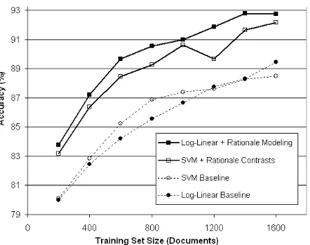
We report on two sets of experiments. In the first set, we use the annotation data that A3–A5 provided for the small set of 100 documents (as well as the data from A0 on those same 100 documents). In the second set, we used A0’s abundant annotation data to evaluate our method with training set sizes up to 1600 documents, and compare it with three other methods: log-linear baseline, SVM baseline, and the SVM masking method of (Zaidan et al., 2007).
7.1 Learning curves
The learning curves reported in section 8.1 are gen-erated exactly as in (Zaidan et al., 2007). Each curve shows classification accuracy at training set sizes
T = 1,2, ...,9folds (i.e. 200,400, ...,1600training documents). For a given sizeT, the reported accu-racy is an average of 9 experiments with different subsets of the entire training set, each of sizeT:
1 9
8
X
i=0
acc(F9 |Fi+1∪. . .∪Fi+T) (5)
whereFj denotes the fold numberedjmod 9, and
acc(F9 | Y) means classification accuracy on the
held-out test setF9after training on setY.
We use an appropriate paired permutation test, de-tailed in (Zaidan et al., 2007), to test differences in (5). We call a difference significant atp <0.05.
7.2 Comparison to “masking SVM” method
We compare our method to the “masking SVM” method of (Zaidan et al., 2007). Briefly, that method used rationales to construct several so-called con-trast examplesfrom every training example. A con-trast example is obtained by “masking out” one of the rationales highlighted to support the training ex-ample’s class. Agood classifier should have more trouble on this modified example. Hence, Zaidan et al. (2007) required the learned SVM to classify each contrast example with a smaller margin than the cor-responding original example (and did not require it to be classified correctly).
[image:8.612.316.540.53.230.2]The masking SVM learner relies on a simple geo-metric principle; is trivial to implement on top of an existing SVM learner; and works well. However, we believe that the generative method we present here is more interesting and should apply more broadly.
Figure 3: Classification accuracy curves for the 4 meth-ods: the two baseline learners that only utilize class data, and the two learners that also utilize rationale annota-tions. The SVM curves are from (Zaidan et al., 2007).
First, the masking method is specific to improving an SVM learner, whereas our method can be used to improve any classifier by adding a rationale-based regularizer (the second half of equation (4)) to its objective function during training.
More important, there are tasks where it is unclear how to generate contrast examples. For the movie review task, it was natural to mask out a rationale by pretending its words never occurred in the doc-ument. After all, most word types do not appear in most documents, so it is natural to consider the non-presence of a word as a “default” state to which we can revert. But in an image classification task, how should one modify the image’s features to ignore some spatial region marked as a rationale? There is usually no natural “default” value to which we could set the pixels. Our method, on the other hand, elim-inates contrast examples altogether.
8 Experimental Results and Analysis
8.1 The added benefit of rationales
Fig. 3 shows learning curves for four methods. A log-linear model shows large and significant im-provements, at all training sizes, when we incor-porate rationales into its training via equation (4). Moreover, the resulting classifier consistently out-performs17 prior work, the masking SVM, which starts with a slightly better baseline classifier (an SVM) but incorporates the rationales more crudely.
17
size A0 A3 A4 A5 SVM baseline 100 72.0 72.0 72.0 70.0 SVM+contrasts 100 75.0 73.0 74.0 72.0 Log-linear baseline 100 71.0 73.0 71.0 70.0 Log-linear+rats 100 76.0 76.0 77.0 74.0
[image:9.612.328.523.57.121.2]SVM baseline 20 63.4 62.2 60.4 62.6 SVM+contrasts 20 65.4 63.4 62.4 64.8 Log-linear baseline 20 63.0 62.2 60.2 62.4 Log-linear+rats 20 65.8 63.6 63.4 64.8
Table 1: Accuracy rates using each annotator’s data. In a given column, a value initalicsis not significantly differ-ent from the highest value in that column, which is bold-faced. The size=20 results average over 5 experiments.
To confirm that we could successfully model an-notators other than A0, we performed the same comparison for annotators A3–A5; each had pro-vided class and rationale annotations on a small 100-document training set. We trained a separateφfor each annotator. Table 1 shows improvements over baseline, usually significant, at 2 training set sizes.
8.2 Analysis
Examining the learned weightsφ~ gives insight into annotator behavior. High weights includeI-O and
O-I transitions conditioned on punctuation, e.g.,
φI(.)-O = 3.55,18 as well as rationales ending at the
end of a major phrase, e.g.,φI-O/E=VP= 1.88. The large emission feature weights, e.g., φrel =
14.68 andφantirel = 15.30, tie rationales closely to
θ values, as hoped. For example, in Figure 1, the word w = succeeds, with θw = 0.13, drives up
p(I)/p(O)by a factor of 7 (in a positive document) relative to a word withθw = 0.
In fact, feature ablation experiments showed that almost all the classification benefit from rationales can be obtained by using only these 2 emission
φ-features and the 4 unconditioned transition φ -features. Our fullφ(115 features) merely improves our ability to predict the rationales (whose likeli-hood does increase significantly with more features). We also checked that annotators’ styles differ enough that it helps to tuneφto the “target” annota-torAwho gave the rationales. Table 3 shows that aφ
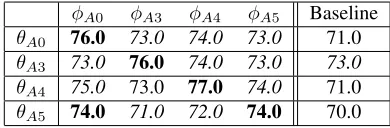
model trained onA’sownrationales does best at pre-dicting new rationales fromA. Table 2 shows that as
18
When trained on foldsF4–F8with A0’s rationales.
[image:9.612.71.308.58.174.2]φA0 φA3 φA4 φA5 Baseline θA0 76.0 73.0 74.0 73.0 71.0 θA3 73.0 76.0 74.0 73.0 73.0 θA4 75.0 73.0 77.0 74.0 71.0 θA5 74.0 71.0 72.0 74.0 70.0
Table 2: Accuracy rate for an annotator’sθ (rows) ob-tained when using some other annotator’sφ (columns). Notice that the diagonal entries and the baseline column are taken from rows of Table 1 (size=100).
Trivial
φA0 φA3 φA4 φA5 model
−L(rA0) 0.073 0.086 0.077 0.088 0.135
−L(rA3) 0.084 0.068 0.071 0.068 0.130
−L(rA4) 0.088 0.084 0.075 0.085 0.153
−L(rA5) 0.058 0.044 0.047 0.044 0.111
Table 3: Cross-entropy per tag of rationale annotations
~r for each annotator (rows), when predicted from that annotator’s ~xand~θ via a possibly different annotator’s
φ(columns). For comparison, the trivial model is a bi-gram model of~r, which is trained on the target annotator but ignores~xand~θ. 5-fold cross-validation on the 100-document set was used to prevent testing on training data.
a result, classification performance on the test set is usually best if it wasA’sownφthat was used to help learnθfromA’s rationales. In both cases, however, a different annotator’sφis better than nothing.
9 Conclusions
We have demonstrated a effective method for elic-iting extra knowledge from naive annotators, in the form of lightweight “rationales” for their an-notations. By explicitly modeling the annotator’s rationale-marking process, we are able to infer a bet-ter model of the original annotations.
We showed that our method performs signifi-cantly better than two strong baseline classifiers, and also outperforms our previous discriminative method for exploiting rationales (Zaidan et al., 2007). We also saw that it worked across four anno-tators who have different rationale-marking styles.
[image:9.612.313.542.188.264.2]References
Eric Brill and Grace Ngai. 1999. Man [and woman] vs. machine: A case study in base noun phrase learning. InProceedings of the 37th ACL Conference.
Michael Collins. 1999. Head-Driven Statistical Models for Natural Language Parsing. Ph.D. thesis, Univer-sity of Pennsylvania.
G. Druck, G. Mann, and A. McCallum. 2008. Learn-ing from labeled features usLearn-ing generalized expecta-tion criteria. InProceedings of ACM Special Interest Group on Information Retrieval, (SIGIR).
A. Haghighi and D. Klein. 2006. Prototype-driven learn-ing for sequence models. In Proceedings of the Hu-man Language Technology Conference of the NAACL, Main Conference, pages 320–327, New York City, USA, June. Association for Computational Linguis-tics.
John Lafferty, Andrew McCallum, and Fernando Pereira. 2001. Conditional random fields: Probabilistic mod-els for segmenting and labeling sequence data. In Pro-ceedings of the International Conference on Machine Learning.
Grace Ngai and David Yarowsky. 2000. Rule writing or annotation: Cost-efficient resource usage for base noun phrase chunking. In Proceedings of the 38th Annual Meeting of the Association for Computational Linguistics, pages 117–125, Hong Kong.
B. Pang and L. Lee. 2004. A sentimental education: Sentiment analysis using subjectivity summarization based on minimum cuts. InProc. of ACL, pages 271– 278.
B. Pang, L. Lee, and S. Vaithyanathan. 2002. Thumbs up? Sentiment classification using machine learning techniques. InProc. of EMNLP, pages 79–86. Hema Raghavan and James Allan. 2007. An interactive
algorithm for asking and incorporating feature feed-back into support vector machines. InProceedings of SIGIR.
Hema Raghavan, Omid Madani, and Rosie Jones. 2006. Active learning on both features and instances. Jour-nal of Machine Learning Research, 7:1655–1686, Aug.
Luis von Ahn, Ruoran Liu, and Manuel Blum. 2006. Peekaboom: A game for locating objects. In CHI ’06: Proceedings of the SIGCHI Conference on Hu-man Factors in Computing Systems, pages 55–64. Omar Zaidan, Jason Eisner, and Christine Piatko. 2007.