Abstract— This article proposes a particle swarm optimization (PSO) technique to address open-shop scheduling problems with multiple objectives. Because PSO was originally formulated to treat continuous optimization problems, we modified the particle position representation, particle velocity, and particle movement to consider the essentially discrete nature of scheduling problems. The modified PSO was tested using two benchmark problems to evaluate its performance. The results demonstrated that the algorithm performed better when only one swarm was used for all three objectives compared to the case where the swarm was divided into three sub-swarms for each objective.
Index Terms— Multi-objective, Open-shop, Particle Swarm Optimization, Scheduling
I. INTRODUCTION
Shop scheduling problems, including flow-, job-, and open-shop problems, have attracted the interest of many researchers. Shop scheduling has become a significant factor used by shops to maintain their competitive position in a rapidly changing marketplace. Most previous research into the open-shop scheduling problem has concentrated on finding a single optimal solution (e.g., makespan). However, in the real world, the multiple-objective requirements of shop scheduling must be achieved simultaneously. Thus, the academic study of open-shop scheduling has been extended from a single objective to multiple objectives.
Because the open-shop scheduling problem is non-deterministic polynomial-time hard (NP-hard) for more than two machines (m > 2) [1], we cannot solve it exactly using a reasonable amount of computation time. Most published research has concentrated on developing heuristic algorithms to search for the optimal makespan of open-shop scheduling problems. A neighborhood search algorithm based on the simulated annealing technique was proposed by Liaw [2] to addresses the problem of scheduling a non-preemptive open shop with the objective of minimizing the makespan. An efficient local search algorithm based on the tabu search technique was also proposed by Liaw [3] to This work was supported by the grant of National Science Council of Taiwan (NSC-96-2221-E-216-052MY3).
D.Y. Sha is with the Chung Hua University, Hsinchu, Taiwan, R.O.C. He is now with the Department of Industrial Engineering and System Management (e-mail: [email protected]).
Hsing-Hung Lin is with National Chiao Tung University, Hsinchu, Taiwan, R.O.C. He is now with the Department of Industrial Engineering and Management (phone: 886-937808216; e-mail: [email protected]).
C.-Y. Hsu is with the Bureau of Employment and Vocational Training of Taiwan, R.O.C.
minimize the makespan.
Liaw [4] developed and applied a hybrid genetic algorithm (HGA) to the open-shop scheduling problem. The hybrid algorithm incorporated a local improvement procedure based on the tabu search (TS) into the basic genetic algorithm (GA). Blum [5] proposed the Beam-ACO technique to tackle open-shop scheduling; this technique consisted of a hybridized solution construction mechanism for ant colony optimization (ACO) with a beam search. Several competitive GAs have also been presented to detect global optimal values disseminated among many quasi-optimal schedules of the open-shop problem [6]. A heuristic technique for the open-shop scheduling problem using the genetic algorithm to minimize the makespan was developed by Senthilkumar and Shahbudeen [7], and Tang and Bai [8] proposed a heuristic algorithm, known as the shortest processing time block (SPTB), to solve the open-shop problem by minimizing the sum of the completion time.
Liaw [9] considered the problem of scheduling preemptive open shops to minimize the total tardiness. He developed an efficient constructive heuristic to solve large problems. To solve medium-sized problems, he proposed a branch-and-bound algorithm that incorporated a lower bound scheme based on the solution of an assignment problem as well as various dominance rules.
Blazewicz et al. [10] applied a non-classical performance measure, the late work criterion, to scheduling problems. They estimated the quality of the obtained solution with regards to the duration of the late parts of the tasks, but did not take into account the quality of these delays.
One of the latest evolutionary techniques, particle swarm optimization (PSO), was recently proposed by Kennedy et al. [11] for unconstrained continuous optimization problems. The idea behind PSO is based on observations of the social behavior of animals such as flocks of birds or schools of fish, combined with swarm theory. PSO has been successfully applied to different fields due to its easy implementation and computational efficiency. Nevertheless, applications of PSO to combinations of optimization problems are still scarce.
The aim of this paper is to explore the development of PSO for elaborate multi-objective open-shop scheduling problems. The original PSO was developed to solve continuous optimization problems; therefore, we modified the particle position representation, particle movement, and particle velocity to accommodate the discrete solution spaces of scheduling optimization problems.
The remainder of this paper is organized as follows. Section 2 contains a formulation of the open-shop scheduling problem with three objectives. Section 3 describes the modified algorithm of the proposed PSO approach. Section 4 contains the simulated results of two benchmark problems. Section 5 provides some conclusions and future directions.
A Modified Particle Swarm Optimization for
Multi-objective Open Shop Scheduling
II. OPEN SHOP SCHEDULING A. Problem Statement
The common characteristics of shop scheduling problems are as follows. A set of n jobs must be processed on a set of m machines. Each job consists of m operations, each of which must be processed on a different machine for a given process time. At any time, at most one operation can be processed on each machine, and at most one operation of each job can be processed. Unlike flow-shop and job-shop scheduling problems, the exceptional condition of the open-shop scheduling problem is that the operations of each job can be processed in any order.
B. Problem Objective
The aim of this study was to assign jobs to machines so that the completion time, also called the makespan, total flow time, and machine idle time are minimized simultaneously. To minimize the makespan, we must minimize the maximum total processing time on all machines. The total flow time refers to the sum of the completion times of all jobs. The idle times of each machine during the work cycle are summed to obtain the total machine idle time.
III. PARTICLE SWARM OPTIMIZATION
PSO is based on observations of the social behavior of animals, such as birds in flocks or fish in schools, as well as on swarm theory. The population consisting of individuals or particles is initialized randomly. Each particle is assigned with a randomized velocity according to its own movement experience and that of the rest of the population. The relationship between the swarm and particles in PSO is similar to the relationship between the population and chromosomes in a GA.
In PSO, the problem solution space is formulated as a search space. Each particle position in the search space is a correlated solution to the problem. Particles cooperate to determine the best position (solution) in the search space (solution space).
Suppose that the search space is D-dimensional and there are ρ particles in the swarm. Particle i is located at position Xi={x1i, x2i, …, xDi} and has velocity Vi={v1i, v2i, …, vDi}, where i=1, 2, …,ρ. Based on the PSO algorithm, each particle move towards its own best position (pbest), denoted as Pbesti={pbest1i, pbest2i,…, pbestni}, and the best position of the whole swarm (gbest) is denoted as Gbest={gbest1, gbest2, …, gbestn} with each iteration. Each particle changes their position according to its velocity, which is randomly generated toward the pbest and gbest positions. For each particle r and dimension s, the new velocity vsr and position xsr of particles can be calculated by the following equations:
] [
] [
1 1 2
2
1 1 1
1 1
− −
− − −
− ×
×
+ − ×
× + × =
τ τ
τ τ τ
τ
rs s
rs rs rs
rs
x gbest rand
c
x pbest rand
c v w v
(1) 1
1 −
− +
= τ τ
τ
rs rs
rs x v
x (2)
In Eqs. (1) and (2), τ is the iteration number. The inertial weight w is used to control exploration and exploitation. A large w value keeps the particles moving at high velocity and prevents them from becoming trapped in local optima. A small w value ensures a low particle velocity and encourages particles to exploit the same search area. The constants c1 and c2 are acceleration coefficients to determine whether particles prefer to move closer to the pbest or gbest positions. The rand1 and rand2 are two independent random numbers uniformly distributed between 0 and 1. The termination criterion of the PSO algorithm includes a maximum number of generations, a designated value of pbest, and lack of further improvement in pbest. The standard PSO process is outlined as follows:
Step 1: Initialize a population of particles with random positions and velocities in a D-dimensional search space.
Step 2: Update the velocity of each particle using Eq. (1). Step 3: Update the position of each particle using Eq. (2). Step 4: Map the position of each particle into the solution space and evaluate its fitness value according to the desired optimization fitness function. Simultaneously update the pbest and gbest positions if necessary.
Step 5: Loop to Step 2 until the termination criterion is met, usually after a sufficient good fitness or a maximum number of iterations.
The original PSO was designed for a continuous solution space. We must modify the PSO position representation, particle velocity, and particle movement so they work better with combinational optimization problems. These changes are described in next section.
IV. METHODS
There are four types of feasible schedules in OSSPs, including inadmissible, semi-active, active, and non-delay. The optimal schedule is guaranteed to be an active schedule. We can decode a particle position into an active schedule employing Giffler and Thompson’s [12] heuristic. There are two different representations of particle position associated with a schedule. The results of Zhang et al.[13] demonstrated that permutation-based position representation outperforms priority-based representation. While choosing to implement permutation-based position presentation, we must also adjust the particle velocity and particle movement.
A. Particle Position Representation
=
k mn k
m k m
k n k
k
k n k
k
k
x x
x
x x
x
x x
x
X
L M M
M
L L
2 1
2 22
21
1 12
11
, wherexijkdenotes the priority
of operationoij, which means the operation of job j that must be processed on machine i.
The Giffler and Thompson (G&T) algorithm is briefly described below.
Notation:
(i,j) is the operation of job j that must be processed on machine i
S is the partial schedule that contains scheduled operations
Ω is the set of operations that can be scheduled
s(i,j) is the earliest time at which operation (i,j) belonging to Ω can be started.
p(i,j) is the processing time of operation (i,j).
f(i,j) is the earliest time at which operation (i,j) belonging to Ω can be finished, f(i,j) = s(i,j) + p(i,j) .
G&T algorithm:
Step 1: Initialize S=φ; Ω to contain all operations without predecessors.
Step 2: Determine f* =min(i,j)∈Ω{f(i,j)}and the machine m* on which f* can be realized.
Step 3:
(1)Identify the operation set (i′,j′)∈Ωsuch that )
,
(i′ j′ requires machine m*, and S(i′,j′)< f*. (2) Choose (i, j) from the operation set identified in Step 3(1) with the largest priority.
(3) Add (i, j) to S.
(4) Assign s(i,j) as the starting time of (i, j). Step 4: If a complete schedule has been generated, stop.
Otherwise, delete (i, j) from Ω, include its immediate successor in Ω, and then go to Step 2.
The movement of particles is modified in accordance with the representation of particle position based on the insertion operator.
B. Particle Velocity
The original PSO velocity concept is that each particle moves according to the velocity determined by the distance between the previous position of the particle and the gbest (pbest) solution. The two major purposes of the particle velocity are to move the particle toward the gbest and pbest solutions, and to maintain the inertia to prevent particles from becoming trapped in local optima.
In the proposed PSO, we concentrated on preventing particles from becoming trapped in local optima rather than
moving them toward the gbest (pbest) solution. If the priority value increases or decreases with the present velocity in this iteration, we maintain the priority value increasing or decreasing at the beginning of the next iteration with probability w, which is the PSO inertial weight. The larger the value of w is, the greater the number of iterations over which the priority value keeps increasing or decreasing, and the greater the difficulty the particle has returning to the current position. For an n-job problem, the velocity of particle k can be represented as
=
k mn k
m k m
k n k
k
k n k
k
k
v v
v
v v
v
v v
v
V
L M L M M
L L
2 1
2 22
21
1 12
11
, where vijk is the
velocity of the operation o of particle k, ij vijk∈{−1,0,1}. The initial particle velocities are generated randomly. Instead of considering the distance from xijk to
)
( ij
k ij gbest
pbest , our PSO considers whether the value of x ijk is larger or smaller than pbestijk(gbestij) If xijk has decreased in the present iteration, this means that
)
( ij
k ij gbest
pbest is smaller than x , and ijk x is set moving ijk toward pbestijk(gbestij) by letting vijk← –1. Therefore, in the next iteration, x is kept decreasing by one (i.e., ijk
k ij
x ←
k ij
x –1) with probability w. Conversely, if x has increased ijk
in this iteration, this means that pbestijk(gbestij) is larger than x , and ijk x is set moving toward ijk pbestijk(gbestij) by letting vijk←1. Therefore, in the next iteration, k
ij
x is kept
increasing by one (i.e. xijk← k ij
x + 1) with probability w.
The inertial weight w influences the velocity of particles in PSO. We randomly update velocities at the beginning of each iteration. For each particle k and operation o , if ij v is not ijk equal to 0, v is set to 0 with probability (1–w). This ensures ijk that x stops increasing or decreasing continuously in this ijk iteration with probability (1–w).
C. Particle Movement
In our PSO, the particle movement is based on the insert operator proposed by Sha and Hsu [14]. We set
5 . 0 2 −
+ ← p rand
xijk if we want to insert o into the pth ij location in the permutation list. In addition, the location of operationo in the operation sequence of kth pbest and gbest ij solution are pbest andijk gbest . When particle k moves, for ij
all oij , if vijk equals 0, the xijk will be set to 5
. 0 2− +rand
pbestijk with probability c1 and set to be 5
. 0 2− +rand
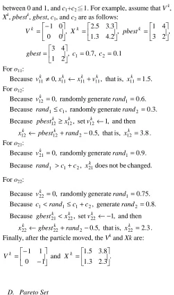
between 0 and 1, and c1+c2≦1. For example, assume that V k, Xk, pbestk, gbest, c1, and c2 are as follows:
1 . 0 , 7 . 0 , 2 1
4 3
, 2 3
4 1
, 2 . 4 3 . 1
3 . 3 5 . 2
, 0 0
0 1
2
1 = =
=
=
= − =
c c
gbest
pbest X
Vk k k
For o11:
Because 11≠0 , 11← 11+ 11, that is, 11 =1.5.
k k
k k k
x v
x x v For o12:
Because v12 =0, randomly generaterand1=0.6.
k
Because rand1 ≤c1, randomly generaterand2 =0.3. Because 12 ≥ 12, set 12 ←1, and then
k k k
v x pbest
12 ← 12+ 2−0.5, that is, 12 =3.8.
k k
k
x rand
pbest x
For o21:
Because v21 =0, randomly generaterand1 =0.9.
k
Because 1 1 2, 21doesnot bechanged.
k
x c c rand > +
For o22:
Because v22 =0, randomly generaterand1 =0.75.
k
Because c1<rand1≤c1+c2, generaterand2 =0.8. Because 21 < 22, set 22 ←−1, and then
k k k
v x gbest
22 ← 22+ 2−0.5, that is, 22 =2.3.
k k
k
x rand
gbest x
Finally, after the particle moved, the Vk and Xk are: .
3 . 2 3 . 1
8 . 3 5 . 1 and 1 0
1 1
=
− −
= k
k X
V
D. Pareto Set
In real world, empirical scheduling decisions should not only involve the deliberation of more than one objective at a time, but also need to prevent the conflict of two or more objectives. The solution set of multi-objective optimization problem with conflicting objective function consisted with the solutions that no other solution is better than all other objective functions is called Pareto optimal. A multi-objective minimization problem with m decision variables and n objectives is given below to describe the concept of Pareto optimality.
The non-dominated solution is defined as solutions which dominate the others but do not dominate themselves. Solution
η is said a Pareto-optimal solution if there exist no other solution ξ in the feasible space which could dominate η. The set including all Pareto-optimal solutions is termed the Pareto-optimal Set, or the efficient set. The graph plotted using collected Pareto-optimal solutions in feasible space is designated as Pareto front.
The external Pareto optimal set is employed to deposit a limited size of non-dominated solutions. Maximum size of archive set is specified in advance. This method is applied to forbid missing fragment of non-dominated front during the searching process. The Pareto-optimal front is getting formed as archive updated iteratively. While the archive set is empty enough and a new non-dominated solution is detected, the new solution will enter the archive set. As the new solution
enters the archive set, any solution in the archive set dominated by this solution will be withdrawn from the archive set. In case the maximum archive size reaches its preset value, the archive set have to decide which solution could be replaced. In this study, we propose a novel Pareto archive set updating process in order to preclude from losing non-dominated solutions when the Pareto archive set is full. When a new non-dominated solution is discovered, the archive set would be updated when one of the following situation occurs: (i) number of solutions in the archive set is less than the maximum value; (ii) number of the solutions in the archive set is equal to (or greater than) the maximum value, then one of the solutions in the archive set that is most dissimilar to the new solution will be replaced by the new solution. We measure the dissimilarity by Euclidean distance. A longer distance implies a higher dissimilarity. The non-dominated solution in the Pareto archive set with the longest distance to the new found solution will be replaced.
V. COMPUTATIONAL EXPERIMENTS A. Experiment Condition
The proposed multi-objective PSO (MOPSO) algorithm was tested on two benchmark problems obtained from Guéret and Prins [15]. The program was coded in Visual C++, and each problem was run 40 times on a Pentium 4 3.0-GHz computer with 1 GB of RAM running Windows XP. During a preliminary experiment, we used four swarm sizes (N = 30, 60, 80, and 100) to test the algorithm. The outcome of N = 80 was best, so that value was used in all further tests. The parameters c1 and c2 were tested at various values in the range 0.1–0.7 at increments of 0.2. The inertial weight w was reduced from wmax to wmin during the iterations, where wmax was set to 0.5, 0.7, and 0.9, and wmin was set to 0.1, 0.3, and 0.5. The combination of c1 = 0.7, c2 = 0.1, wmax = 0.7, and wmin = 0.3 gave the best results. The maximum iteration limit was set to 60, and the maximum archive size was set to 80.
B. Experiment Results
In the first experiment, we assigned the Pareto set to the Pbest solutions and considered four different conditions (see Table 1). In the first scenario, we took all three objectives into consideration. Only two objectives, the makespan and total flow time, were considered in the second scenario. The third and fourth scenarios considered the makespan and machine idle time, and the total flow time and machine idle time, respectively. The results of the first experiment are listed in Table 1.
[image:4.595.43.294.45.470.2]used for the object total flow time and machine idle time objectives.
Table 1 Results of the first experiment makespane total flow time
machine idle time Optimized
Objectives best Ave. best Ave. best Ave.
All 1092.4 1099.38 10575.1 10643.31 592.6 662.63
MS+TFT 1093.5 1098.98 10576.0 10639.25 631.6 697.62
MS+MIT 1090.8 1098.96 10619.4 10695.07 585.2 651.37
TFT+MIT 1097.0 1105.85 10564.5 10638.14 568.4 646.97
M: makespan, TFT: total flow time, MIT: machine idle time
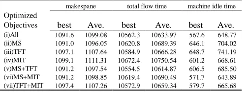
Table 2 Results of the second experiment
makespane total flow time machine idle time Optimized
Objectives best Ave. best Ave. best Ave.
(i)All 1091.6 1099.08 10562.3 10633.97 567.6 648.77 (ii)MS 1091.0 1096.05 10620.8 10689.39 646.1 704.02 (iii)TFT 1097.1 1107.64 10584.9 10666.28 648.7 741.19 (iv)MIT 1099.1 1111.31 10672.4 10750.54 601.2 668.61 (v)MS+TFT 1091.2 1097.54 10554.5 10614.87 606.5 685.50 (vi)MS+MIT 1091.2 1098.85 10619.4 10690.49 571.7 643.89 (vii)TFT+MIT 1097.4 1107.26 10572.9 10659.34 579.7 665.68
VI. CONCLUSION
Although a large amount of research has addressed the open-shop scheduling problem, most of this has focused on minimizing the maximum completion time (i.e., makespan). Other objectives exist in the real world, such as minimizing the machine idle time, that might help improve efficiency and reduce production costs. PSO, inspired by the behavior of flocks of birds and schools of fish, has the advantages of a simple structure, easy implementation, immediate accessibility, short search time, and robustness. However, few applications of PSO to multi-objective open-shop scheduling problems can be found in the literature. Therefore, we proposed a MOPSO algorithm to solve the open-shop scheduling problem with multiple objectives, including minimization of makespan, total flow time, and machine idle time.
The original PSO was developed for continuous optimization problems. To make it suitable for job-shop scheduling (i.e., a combinational problem), we modified the representation of particle position, particle movement, and particle velocity. We also introduced a Pareto set and used a diversification strategy.
The algorithm was tested to verify different scenarios, using different Pareto sets with different combinations of objectives. Different swarm sizes with varied objective combinations were also evaluated. The results demonstrated that the algorithm performed better when only one swarm was used for all three objectives compared to the case where the swarm was divided into three sub-swarms for each objective. We will attempt to apply MOPSO to other shop scheduling problems with multiple objectives in future research. Other possible topics for further study include modification of the particle position, particle movement, and particle velocity representation. Issues related to Pareto optimization, such as solution maintenance strategy and performance measurement, also merit future investigation.
APPENDIX
A pseudo-code of the PSO for MO-OSSP is as follow. Initialize a population of particles with random positions.
for each particle k do
Evaluate Xk (the position of particle k) Save the pbestk to optimal solution set S end for
Set gbest solution equals to the best pbestk repeat
Updates particles velocities for each particle k do Move particle k
Evaluate Xk
Update gbest, pbest and S end for
until maximum iteration limit is reached
REFERENCES
[1] Gonzalez T., Sahni S., “Open shop scheduling to minimize finish time,” Journal of the ACM, Vol. 23, 1976, pp. 665–79.
[2] Liaw C.-F., “Applying simulated annealing to the open shop scheduling problem,” IIE Transactions, Vol. 31, 1999, pp. 457–65. [3] Liaw C.-F., “A tabu search algorithm for the open shop scheduling
problem,” Computers & Operations Research, Vol.26, 1999, pp. 109–26.
[4] Liaw C.-F., “A hybrid genetic algorithm for the open shop scheduling problem,” European Journal of Operational Research, Vol.124, 2000, pp. 28–42.
[5] Blum C., “Beam-ACO—Hybridizing ant colony optimization with beam search: an application to open shop scheduling,” Computers &
Operations Research, Vol. 32, 2005, pp. 1565–91.
[6] Prins C., “Competitive genetic algorithms for the open-shop scheduling problem,” Mathematical Methods of Operations Research, Vol. 52, 2000, pp. 389–411.
[7] Senthilkumar P., Shahbudeen P., “GA based heuristic for the open job shop scheduling problem,” International Journal of Advanced
Manufacturing Technology, Vol. 30, 2006, pp. 297–301.
[8] Tang L., Bai D., “A new heuristic for open shop total completion time problem,” Applied Mathematical Modeling, vol. 34 2010, pp. 735–743.
[9] Liaw C.-F., “Scheduling preemptive open shops to minimize total tardiness,” European Journal of Operational Research, Vol.162, 2005, pp. 173–183.
[10] Bllzewicz J., Pesch E., Sterna M., Werner F., “Open shop scheduling problems with late work criteria,” Discrete Applied Mathematics, Vol. 134, 2004, pp. 1–24.
[11] Kennedy J, Eberhart R.C., “Particle swarm optimization,” Proceedings
of the 1995 IEEE International Conference on Neural Networks. New
Jersey: IEEE Press; 1995, pp. 1942–8.
[12] Giffler J, Thompson G.L., “Algorithms for solving production scheduling problems,” Operations Research, Vol. 8, 1960, pp. 487–503.
[13] Zhang H., Li H., Tam C.M., “Particle swarm optimization for resource-constrained project scheduling,” International Journal of
Project Management, Vol. 24, 2006, pp. 83–92.
[14] Sha D.Y., Hsu C.-Y., “A new particle swarm optimization for the open shop scheduling problem,” Computers & Operations Research, Vol. 35, 2008, pp. 3243–3261.
[15] Guéret C., Prins C., “A new lower bound for the open-shop problem,”