Modeling Category Structures with a Kernel Function
Hiroya Takamura
Precision and Intelligence Laboratory
Tokyo Institute of Technology
4259 Nagatsuta Midori-ku Yokohama,
226-8503 Japan
[email protected]
Yuji Matsumoto
Department of Information Technology
Nara Institute of Science and Technology
8516-9 Takayama Ikoma Nara,
630-0101 Japan
[email protected]
Hiroyasu Yamada
School of Information Science
Japan Advanced Institute of Science and Technology
1-1 Asahidai Tatsunokuchi Ishikawa, 923-1292 Japan
[email protected]
Abstract
We propose one type of TOP (Tangent vector Of the Posterior log-odds) kernel and apply it to text categorization. In a number of categoriza-tion tasks including text categorizacategoriza-tion, nega-tive examples are usually more common than positive examples and there may be several dif-ferent types of negative examples. Therefore, we construct a TOP kernel, regarding the prob-abilistic model of negative examples as a mix-ture of several component models respectively corresponding to given categories. Since each component model of our mixture model is ex-pressed using a one-dimensional Gaussian-type function, the proposed kernel has an advantage in computational time. We also show that the computational advantage is shared by a more general class of models. In our experiments, the proposed kernel used with Support Vector Machines outperformed the linear kernel and the Fisher kernel based on the Probabilistic La-tent Semantic Indexing model.
1
Introduction
Recently, Support Vector Machines (SVMs) have been actively studied because of their high generalization abil-ity (Vapnik, 1998). In the formulation of SVMs, func-tions which measure the similarity of two examples take an important role. These functions are called kernel
func-tions. The usual dot-product of two vectors respectively
corresponding to two examples is often used. Although some variants to the usual dot-product are sometimes used (for example, higher-order polynomial kernels and RBF kernels), the distribution of examples is not taken into account in such kernels.
However, new types of kernels have more recently been proposed; they are based on the probability distri-bution of examples. One is Fisher kernels (Jaakkola and Haussler, 1998). The other is TOP (Tangent vector Of the Posterior log-odds) kernels (Tsuda et al., 2002). While Fisher kernels are constructed on the basis of a genera-tive model of data, TOP kernels are based on the class-posterior probability, that is, the probability that the pos-itive class occurs given an example. However, in order to use those kernels, we have to select a probabilistic model of data. The selection of a model will affect categoriza-tion result. The present paper provides one solucategoriza-tion to this issue. Specifically, we proposed one type of TOP kernel, because it has been reported that TOP kernels per-form better than Fisher kernels in terms of categorization accuracy.
Hyperplane-based TOP (HP-TOP) kernel, can be
com-puted efficiently in spite of its high dimensionality. We later show that the computational advantage is shared by a more general class of models.
In the experiments of text categorization, in which SVMs are used as classifiers, our kernel outperformed the linear kernel and the Fisher kernel based on the Prob-abilistic Latent Semantic Indexing model proposed by Hofmann (2000) in terms of categorization accuracy.
2
SVMs and Kernel Method
In this section, we explain SVMs and the kernel method, which are the basis of our research. SVMs have achieved high accuracy in various tasks including text categoriza-tion (Joachims, 1998; Dumais et al., 1998).
Suppose a setDlof ordered pairs consisting of a fea-ture vector and its label
Dl= {(x
1, y1),(x2, y2),· · ·,(xl, yl)},
(∀i, xi∈R|I|, yi∈ {−1,1}) (1)
is given.Dlis called training data.Iis the set of feature
indices. In SVMs, a separating hyperplane (f(x) = w· x−b) with the largest margin (the distance between the hyperplane and its nearest vectors) is constructed.
Skipping the details of SVMs’ formulation, here we just show the conclusion that, using some real numbers α∗
i (∀i)andb∗, the optimal hyperplane is expressed as
follows:
f(x) =X
i
α∗iyixi·x−b∗. (2)
We should note that only dot-products of examples are used in the above expression.
Since SVMs are linear classifiers, their separating abil-ity is limited. To compensate for this limitation, the
kernel method is usually combined with SVMs (Vapnik,
1998).
In the kernel method, the dot-products in (2) are re-placed with more general inner-products K(xi,x)(kernel functions). The polynomial kernel(xi·xj+1)d(d∈N+) and the RBF kernel exp{−kxi −xjk2/2σ2} are often
used. Using the kernel method means that feature vectors are mapped into a (higher dimensional) Hilbert space and linearly separated there. This mapping structure makes non-linear separation possible, although SVMs are basi-cally linear classifiers.
Another advantage of the kernel method is that al-though it deals with a high dimensional (possibly infinite) space, explicit computation of high dimensional vectors is not required. Only the general inner-products of two vectors need to be computed. This advantage leads to a relatively small computational overhead.
3
Kernels from Probabilistic Models
Recently new type of kernels which connect genera-tive models of data and discriminagenera-tive classifiers such as SVMs, have been proposed: the Fisher kernel (Jaakkola and Haussler, 1998) and the TOP (Tangent vector Of the Posterior log-odds) kernel (Tsuda et al., 2002).
3.1 Fisher Kernel
Suppose we have a probabilistic generative modelp(x|θ)
of the data (we denote an example by x). The Fisher score of x is defined as∇θlogp(x|θ), where ∇θ means
par-tial differentiation with respect to the parametersθ. The Fisher information matrix is denoted byI(θ) (this ma-trix defines the geometric structure of the model space). Then, the Fisher kernel at an estimateθˆis given by:
K(x1,x2)
= (∇θlogp(x1|θˆ))tI−1(ˆθ)(∇θlogp(x2|θˆ)) (3)
The Fisher score of an example approximately indicates how the model will change if the example is added to the training data used in the estimation of the model. That means, the Fisher kernel between two examples will be large, if the influences of the two examples to the model are similar and large (Tsuda and Kawanabe, 2002).
The matrixI(θ)is often approximated by the identity matrix to avoid large computational overhead.
3.2 TOP Kernel
On the basis of a probabilistic model of the data, TOP kernels are designed to extract feature vectors fθˆwhich are considered to be useful for categorization with a sep-arating hyperplane.
We begin with the proposition that, between the gener-alization errorR(fθˆ)and the expected error of the poste-rior probabilityD(fˆθ), the relationR(fθˆ)−L∗≤2D(fθˆ) holds, whereL∗is the Bayes error. This inequality means
that minimizingD(fθˆ)leads to reducing the generaliza-tion error R(fθˆ). D(fˆθ) is expressed, using a logistic
functionF(t) = 1/(1 + exp(−t)), as D(fθˆ)
= min
w,bEx|F(w·fθˆ−b)−P(y= +1|x, θ
∗)|, (4)
where θ∗ denotes the actual parameters of the model. The TOP kernel consists of features which can minimize D(fθˆ). In other words, we would like to have feature vec-tors fθˆthat satisfy the following:
∀x, w·fθˆ(x)−b=F−1(P(y= +1|x, θ∗)). (5) for certain values of w andb.
For that purpose, we first define a functionv(x, θ):
v(x, θ)≡F−1(P(y= +1|x, θ))
The first-order Taylor expansion of v(x, θ∗)around the estimateθˆis
v(x, θ∗)≈v(x,θˆ) +
X
i
(θ∗
i −θˆi)
∂v(x,θˆ)
∂θi
. (7)
If fθˆis of the following form:
fθˆ(x) = ¡
v(x,θˆ), ∂v(x,θˆ)/∂θ1,· · ·, ∂v(x,θˆ)/∂θp ¢
, (8) and if w andbare properly chosen as
w= (1, θ∗
1−θˆ1,· · ·, θp∗−θˆp), b= 0, (9)
then (5) is approximately satisfied. Thus, the TOP kernel is defined as
K(x1,x2) =fθˆ(x1)·fθˆ(x2). (10)
A detailed discussion of the TOP kernel and its theoreti-cal analysis have been given by Tsuda et al (Tsuda et al., 2002).
4
Related Work
Hofmann (2000) applied Fisher kernels to text catego-rization under the Probabilistic Latent Semantic Indexing (PLSI) model (Hofmann, 1999).
In PLSI, the joint probability of document d and word wis :
P(d, w) =
X
k
P(zk)P(d|zk)P(w|zk), (11)
where variables zk correspond to latent classes. After
the estimation of the model using the EM algorithm, the Fisher kernel for this model is computed. The average log-likelihood of document d normalized by the docu-ment length is given by
l(d) =X
j
ˆ
P(wj|d) log X
k
P(wj|zk)P(zk|d), (12)
where ˆ
P(wj|d) = f req(wj,
d) P
mf req(wm,d).
(13)
They use spherical parameterization (Kass and Vos, 1997) instead of the original parameters in the model. They define parametersρjk = 2
p
P(wj|zk)andρk =
2pP(zk), and obtained
∂l(d) ∂ρjk =
ˆ
P(wpj|d)P(zk|d, wj)
P(wj|zk)
, (14)
∂l(d) ∂ρk ≈
P(zk|d) p
P(zk)
. (15)
Thus, the Fisher kernel for this model is obtained as de-scribed in Appendix A.
The first term of (31) corresponds to the similarity through latent spaces. The second term corresponds to the similarity through the distribution of each word. The number of latent classes zk can affect the value of the
kernel function. In the experiment of (Hofmann, 2000), they computed the kernels with the different numbers (1 to 64) ofzk and added them together to make a robust
kernel instead of deciding one specific number of latent classeszk.
They concluded that the Fisher kernel based on PLSI is effective when a large amount of unlabeled examples are available for the estimation of the PLSI model.
5
Hyperplane-based TOP Kernel
In this section, we explain our TOP kernel.
5.1 Derivation of HP-TOP kernel
Suppose we have obtained the parameters wc and bc
of the separating hyperplane for each category c ∈ Ccategory in the original feature space, whereCcategory
denotes the set of categories.
We assume that the class-posteriors Pc(+1|d) and
Pc(−1|d)are expressed as1
Pc(+1|d) = P(c)q(
d|c) P
c0P(c0)q(d|c0)
, (16)
Pc(−1|d) = P
e6=cP(e)q(d|e) P
c0P(c0)q(d|c0)
(17)
where, for any categoryx, component functionq(d|x)is of Gaussian-type:
q(d|x) = p1 2πσ2
x
exp{−((wx·d−bx)−µx)
2
2σ2 x
}, (18) with the meanµxof a random variable wx·d−bxand
the varianceσx. Those parameters are estimated with the
maximum likelihood estimation, as follows:
µx= P
(d,y)∈Dl,y=x{wx·d−bx}
|{(d,y)∈Dl|y=x}| , (19)
σx= P
(d,y)∈Dl,y=x{wx·d−bx−µx} 2
|{(d,y)∈Dl|y=x}| . (20)
We choose the Gaussian-type function as an exam-ple.However, this choice is open to argument, since some other models also have the same computational advan-tage as described in Section 5.4.
We setθx1 =µx/σ2x,θx2 = −1/2σ2x. Althoughθx1 and θx2 are not the natural parameters of this model,
1
we parameterize this model using the parameters θx1,
θx2, wx, bx and P(x) (∀x ∈ Ccategory) for
simplic-ity. Using this probabilistic model,we compute func-tion v(d, θ) as described in Appendix B (θ denotes {wx, bx, θx1, θx2|x∈Ccategory}andwxidenotes thei
-th element of -the weight vector wx).
The partial derivatives of this function with respect to the parameters are in Appendix C.
Then we can follow the definition (10) to obtain our version of the TOP kernel. We call this new kernel a
hyperplane-based TOP (HP-TOP) kernel.
5.2 Properties of HP-TOP kernel
In the derivatives (39), which provide the largest number of features, original featuresdiare accompanied by other
factors computed from probability distributions. This form suggests that two vectors are considered to be more similar, if they have similar distributions over categories. In other words, an occurrence of a word can have dif-ferent contribution to the classification result, depending on the context (i.e., the other words in the document). This property of the HP-TOP kernel can lead to the ef-fect of word sense disambiguation, because “bank” in a financial document is treated differently from “bank” in a document related to a river-side park.
The derivatives (34) and (35) correspond to the first-order differences, respectively for the positive class and the negative class. Similarly, the derivatives (36) and (37) for the second-order differences. The derivatives (40) and (41) are for the first-order differences normalized by the variances.
The derivatives other than (38) and (38) directly de-pend on the distance from a hyperplane, rather than on the value of each feature. These derivatives enrich the feature set, when there are few active words, by which we mean the words that do not occur in the training data. For this reason, we expect that the HP-TOP kernel works well for a small training dataset.
5.3 Computational issue
Computing the kernel in this form is time-consuming, be-cause the number of components of type (39) can be very large:
O(|I| × |Ccategory|), (21)
whereIdenotes the set of indices for original features. However, we can avoid this heavy computational cost as follows. Let us compute the dot-product of deriva-tives (39) of two vectors d1 and d2, which is shown in Appendix D. The last expression (45) is regarded as the scalar product of two dot-products. Thus, by preserving vectors d and
Ã
−P(e)q(d|e) P−c(d)
µe−(we·d−be)
σ2 e
!
e6=c,e∈Ccategory ,(22)
we can efficiently compute the dot-product in (39); the computational complexity of a kernel function is
O(|I|), (23)
on the condition that the original dimension is larger than the number of categories. Thus, from the viewpoint of computational time, our kernel has an advantage over some other kernels such as the PLSI-based Fisher kernel in Section 4, which requires the computational complex-ity ofO(|I| × |Ccluster|), whereCclusterdenotes the set
of clusters.
In the PLSI-based Fisher kernel, each word has a prob-ability distribution over latent classes. In this sense, the PLSI-based Fisher kernel is more detailed, but detailed models are sometimes suffer overfitting to the training data and have the computational disadvantage as men-tioned above.
The PLSI-based Fisher kernel can be extended to a TOP kernel by using given categories as latent classes. However, the problem of computational time still re-mains.
5.4 General statement about the computational advantage
So far, we have discussed the computational time for the kernel constructed on the Gaussian mixture. How-ever, the computational advantage of the kernel, in fact, is shared by a more general class of models.
We examine the required conditions for the computa-tional advantage. Suppose the class-posteriors have the mixture form as Equations (16) and (17), but function q(d|x)does not have to be a Gaussian-type function. In-stead, functionq(d|x)is supposed to be represented using some functionrparametrized by weandb, as:
q(d|x) = r(fx(d)|x), (24)
wherefx is a scalar function. Then, let us obtain the
derivative ofv(d, θ)with respect towei, which is the
bot-tleneck of kernel computation:
∂v(d, θ)
∂wei
= −P(e)q(d|e) P−c(d)
∂r(fe(d)|e)
∂wei
= −P(e)q(d|e) P−c(d)
∂r(fe(d)|e)
∂fe(d)
∂fe(d)
∂wei
. (25)
The first two factors of (25) do not depend oni. There-fore, if the last factor of (25) is variable-separable with respect toeandi:
∂fe(d)
∂wei
where S andT are some function, then the derivative (25) is also variable-separable. In such cases, the effi-cient computation described in Section 5.3 is possible by preserving the vectors:
¡
T(i)¢i∈I, (27) Ã
−PP(e)q(d|e)
−c(d)
∂r(fe(d)|e)
∂fe(d) S(e)
!
e6=c,e∈Ccategory .(28)
We have now obtained the required conditions for the efficient computation: Equation (24) and the variable-separability.
In case of Gaussian-type functions, functionfeand its
derivative with respect toweiare
fe(d) = we·d−be, (29)
∂fe(d)
∂wei = di.
(30)
Thus, the conditions are satisfied.
6
Experiments
Through experiments of text categorization, we empiri-cally compare the HP-TOP kernel with the linear kernel and the PLSI-based Fisher kernel. We use Reuters-21578 dataset2with ModApte-split (Dumais et al., 1998). In ad-dition, we delete some texts from the result of ModApte-split, because those texts have no text body. After the deletion, we obtain 8815 training examples and 3023 test examples. The words that occur less than five times in the whole training set are excluded from the original feature set.
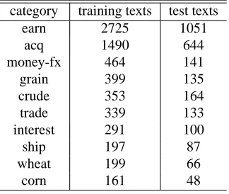
We do not use all the 8815 training examples. The size of the actual training data ranges from 1000 to 8000. For each dataset size, experiments are executed 10 times with different training sets.The result is evaluated with F-measures for the most frequent 10 categories (Table 1). The total number of categories is actually 116. How-ever, for small categories, reliable statistics cannot be ob-tained. For this reason, we regard the remaining cate-gories other than the 10 most frequent catecate-gories as one category. Therefore, the model for negative examples is a mixture of 10 component models (9 out of the 10 most frequent categories and the new category consisting of the remaining categories).
We assume uniform priors for categories as in (Tsuda et al., 2002). We computed the Fisher kernels with differ-ent numbers (10, 20 and 30) of latdiffer-ent classes and added them together to make a robust kernel (Hofmann, 2000). After the learning in the original feature space, the param-eters for the probability distributions are estimated with
2
Available from
[image:5.612.347.509.97.234.2]http://www.daviddlewis.com/resources/.
Table 1: The categories and their sizes of Reuters-21578
category training texts test texts
earn 2725 1051
acq 1490 644
money-fx 464 141
grain 399 135
crude 353 164
trade 339 133
interest 291 100
ship 197 87
wheat 199 66
corn 161 48
maximum likelihood estimation as in Equations (19) and (20), followed by the learning with the proposed kernel.
We used an SVM package, TinySVM3, for SVM com-putation. The soft-margin parameterC was set to 1.0 (other values ofC showed no significant changes in re-sults).
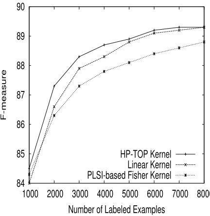
The result is shown in Figure 1 (for macro-average) and Figure 2 (for micro-average). The HP-TOP kernel outperforms the linear kernel and the PLSI-based Fisher kernel for every number of examples.
At each number of examples, we conducted a Wilcoxon Signed Rank test with 5% significance-level, for the HP-TOP kernel and the linear kernel, since these two are better than the other. The test shows that the dif-ference between the two methods is significant for the training data sizes 1000 to 5000. The superiority of the HP-TOP kernel for small training datasets supports our expectation that the enrichment of feature set will lead to better performance for few active words. Although we also expected that the effect of word sense disambigua-tion would improve accuracy for large training datasets, the experiments do not provide us with an empirical ev-idence for the expectation. One possible reason is that Gaussian-type functions do not reflect the actual distribu-tion of data. We leave its further investigadistribu-tion as future research.
In this experimental setting, the PLSI-based Fisher ker-nel did not work well in terms of categorization accuracy. However, this Fisher kernel will perform better when the number of labeled examples is small and a number of unlabeled examples are available, as reported by Hof-mann (2000).
We also measured computational time of each method (Figure 3). The vertical axis indicates the average com-putational time over 100 runs of experiments (10 runs for each category). Please note that training time in this
fig-3
Available from
64
66
68
70
72
74
76
78
80
82
1000 2000 3000 4000 5000 6000 7000 8000
F-measure
Number of Labeled Examples
HP-TOP Kernel
[image:6.612.322.533.78.300.2]Linear Kernel
PLSI-based Fisher Kernel
Figure 1: Macro-average of F-measure
84
85
86
87
88
89
90
1000 2000 3000 4000 5000 6000 7000 8000
F-measure
Number of Labeled Examples
HP-TOP Kernel
[image:6.612.76.292.143.361.2]Linear Kernel
PLSI-based Fisher Kernel
Figure 2: Micro-average of F-measure
0.1
1
10
100
1000
10000
1000 2000 3000 4000 5000 6000 7000 8000
Computational Time (seconds)
[image:6.612.76.292.408.630.2]Number of Labeled Examples
HP-TOP Kernel
Linear Kernel
PLSI-based Fisher Kernel
Figure 3: Computational time of each method
ure does not include the computational time required for feature extraction4. This result empirically shows that the HP-TOP kernel outperforms the PLSI-based Fisher ker-nel in terms of computational time as theoretically ex-pected in Section 5.3.
7
Conclusion
We proposed a TOP kernel based on separating hy-perplanes. The proposed kernel is created from one-dimensional Gaussians along the normal directions of the hyperplanes. We showed that the computational advan-tage that the proposed kernel has is shared by a more general class of models. We empirically showed that the proposed kernel outperforms the linear kernel in text cat-egorization.
Although the superiority of the proposed method to the linear kernel was shown, the proposed method has to be further investigated. Firstly, for large data sizes (namely 7000 and 8000), the proposed method was not signifi-cantly better than the linear kernel. The effectiveness of the proposed method should be confirmed by more ex-periments and theoretical analysis. Secondly, we have to compare the proposed method with other kernels in or-der to check the effectiveness of the kernel function con-sisting of one-dimensional Gaussians normal to the hy-perplanes. The use of Gaussians is open to argument, because their symmetric form is somewhat against our
4
intuition.
This model can be extended to incorporate unlabeled examples, for example, using the EM algorithm. In that sense, the combination of PLSI and the semi-supervised EM algorithm is also one promising model. When the category structure of the negative examples is not given, the proposed method is not applicable. We should inves-tigate whether unsupervised clustering can substitute for the category structure.
References
Susan T. Dumais, John Platt, David Heckerman, and Mehran Sahami. 1998. Inductive learning algo-rithms and representations for text categorization. In
Proceedings of the Seventh International Conference on Information and Knowledge Management (ACM-CIKM98), pages 148–155.
Thomas Hofmann. 1999. Probabilistic Latent Seman-tic Indexing. In Proceedings of the 22nd Annual ACM
Conference on Research and Development in Informa-tion Retrieval, pages 50–57, Berkeley, California,
Au-gust.
Thomas Hofmann. 2000. Learning the similarity of doc-uments: An information geometric approach to docu-ment retrieval and categorization. In Advances in
Neu-ral Information Processing Systems, 12, pages 914–
920.
Tommi Jaakkola and David Haussler. 1998. Exploiting generative models in discriminative classifiers. In
Ad-vances in Neural Information Processing Systems 11,
pages 487–493.
Thorsten Joachims. 1998. Text categorization with sup-port vector machines: Learning with many relevant features. In Proceedings of the 10th European
Con-ference on Machine Learning, pages 137–142.
Robert E. Kass and Paul W. Vos. 1997. Geometrical
foundations of asymptotic inference. New York :
Wi-ley.
Koji Tsuda and Motoaki Kawanabe. 2002. The leave-one-out kernel. In Proceedings of International
Con-ference on Artificial Neural Networks, pages 727–732.
Koji Tsuda, Motoaki Kawanabe, Gunnar R¨atsch, S¨oren Sonnenburg, and Klaus-Robert M¨uller. 2002. A new discriminative kernel from probabilistic models.
Neu-ral Computation, 14(10):2397–2414.
Vladimir Vapnik. 1998. Statistical Learning Theory.
A
Fisher Kernel based on PLSI
K(d1,d2) = X k
P(zk|d1)P(zk|d2)
P(zk) +
X
j ˆ
P(wj|d1) ˆP(wj|d2)
X
k
P(zk|d1, wj)P(zk|d2, wj)
P(wj|zk) , (31)
where P(zk|d, wj) = PP(zk)P(d|zk)P(wj|zk) lP(zl)P(d|zl)P(wj|zl)
Ã
=P(zk)P(d|zk)P(wj|zk)
P(d, wj)
!
. (32)
B
Function
v
for HP-TOP Kernel
v(d, α,w, b) = logP(+1|d)−logP(−1|d)
= logPP(c)q(d|c) c0P(c0)q(d|c0)
−log
P
e6=cP(e)q(d|e)
P
c0P(c0)q(d|c0)
= logP(c)q(d|c)−log
X
e6=c
P(e)q(d|e)
= logP(c) exp{θc1(wc·d) +θc2(wc·d)2+ θ 2 c1 4θc2
−1
2log
−π θc2
}
−logX e6=c
P(e) exp{θe1(we·d) +θe2(we·d)2+ θ 2 e1 4θe2
−1
2log
−π θe2
}, (33)
whereθx1=µx/σ2x, θx2=−1/2σ2x.
C
Partial Derivatives
∂v(d, θ)
∂θc1 = wc·d−bc−µc, (34)
∂v(d, θ)
∂θe1
= −P P(e)q(d|e)
c06=cP(c0)q(d|c0)
(we·d−be−µe), (35)
∂v(d, θ)
∂θc2
= (wc·d−bc)2−µ2c−σc2, (36)
∂v(d, θ)
∂θe2 = −
P(e)q(d|e)
P
c06=cP(c0)q(d|c0)
{(we·d−be)2−µ2e−σ2e}, (37)
∂v(d, θ)
∂wci =
µc−(wc·d−bc)
σ2
c di, (38)
∂v(d, θ)
∂wei = −
P(e)q(d|e)
P
c06=cP(c0)q(d|c0)
µe−(we·d−be)
σ2
e di, (39)
∂v(d, θ)
∂bc =
wc·d−bc−µc
σ2
c , (40)
∂v(d, θ)
∂be
= −P P(e)q(d|e)
c06=cP(c0)q(d|c0)
we·d−be−µe
σ2 e
, (41)
∂v(d, θ)
P(c) = 1
P(c), (42)
∂v(d, θ)
P(e) = −
P(d|e)
P
c06=cP(c0)q(d|c0)
. (43)
D
Dot-product of Derivatives (39) in Appendix C
X
e6=c
X
i
∂v(d1, θ)
∂wei
∂v(d2, θ)
∂wei
= X
e6=c
X
i
P(e)2q(
d1|e)q(d2|e)
P−c(d1)P−c(d2)
µe−(we·d−be)
σ2 e
µe−(we·d−be)
σ2 e
d1
id2i (44)
= µX
e6=c
P(e)2q(
d1|e)q(d2|e)
P−c(d1)P−c(d2)
µe−(we·d−be)
σ2 e
µe−(we·d−be)
σ2 e
d1·d2, (45)