Making Asynchronous Stochastic Gradient Descent Work for Transformers

Proceedings of the 3rd Workshop on Neural Generation and Translation (WNGT 2019), pages 80–89 80

Making Asynchronous Stochastic Gradient Descent Work for

Transformers

Alham Fikri Aji and Kenneth Heafield

School of Informatics, University of Edinburgh 10 Crichton Street

Edinburgh EH8 9AB Scotland, European Union

[email protected], [email protected]

Abstract

Asynchronous stochastic gradient descent (SGD) converges poorly for Transformer mod-els, so synchronous SGD has become the norm for Transformer training. This is unfortu-nate because asynchronous SGD is faster at raw training speed since it avoids waiting for synchronization. Moreover, the Transformer model is the basis for state-of-the-art models for several tasks, including machine transla-tion, so training speed matters. To understand why asynchronous SGD under-performs, we blur the lines between asynchronous and syn-chronous methods. We find that summing sev-eral asynchronous updates, rather than apply-ing them immediately, restores convergence behavior. With this method, the Transformer attains the same BLEU score 1.36 times as fast.

1 Introduction

Models based on Transformers (Vaswani et al.,

2017) achieve state-of-the-art results on various machine translation tasks (Bojar et al.,2018). Dis-tributed training is crucial to training these mod-els in a reasonable amount of time, with the dominant paradigms being asynchronous or syn-chronous stochastic gradient descent (SGD). Prior work (Chen et al., 2016, 2018;Ott et al., 2018) commented that asynchronous SGD yields low quality models without elaborating further; we confirm this experimentally in Section2.1. Rather than abandon asynchronous SGD, we aim to repair convergence.

Asynchronous SGD and synchronous SGD have two key differences: batch size and stale-ness. Synchronous SGD increases the batch size in proportion to the number of processors because gradients are summed before applying one update. Asynchronous SGD updates with each gradient as

it arises, so the batch size is the same as on a sin-gle processor. Asynchronous SGD also has stale gradients because parameters may update several times while a gradient is being computed.

To tease apart the impact of batch size and stale gradients, we perform a series of experiments on both recurrent neural networks (RNNs) and Trans-formers manipulating batch size and injecting stal-eness. Out experiments show that small batch sizes slightly degrade quality while stale gradients substantially degrade quality.

To restore convergence, we propose a hybrid method that computes gradients asynchronously, sums gradients as they arise, and updates less of-ten. Gradient summing has been applied to in-crease batch size or reduce communication (Dean et al.,2012;Lian et al.,2015;Ott et al.,2018; Bo-goychev et al.,2018); we find it also reduces harm-ful staleness. In a sense, updating less often in-creases staleness because gradients are computed with respect to parameters that could have been updated. However, if staleness is measured by the number of intervening updates to the model, then staleness is reduced because updates happen less often. Empirically, our hybrid method converges comparably to synchronous SGD, preserves final model quality, and runs faster because processors are not idle.

2 Exploring Asynchronous SGD

2.1 Baseline: The Problem

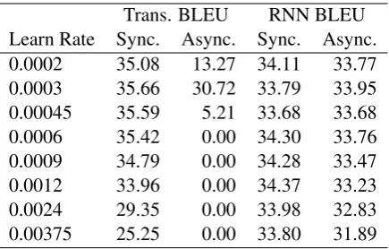
Trans. BLEU RNN BLEU Learn Rate Sync. Async. Sync. Async. 0.0002 35.08 13.27 34.11 33.77 0.0003 35.66 30.72 33.79 33.95 0.00045 35.59 5.21 33.68 33.68 0.0006 35.42 0.00 34.30 33.76 0.0009 34.79 0.00 34.28 33.47 0.0012 33.96 0.00 34.37 33.23 0.0024 29.35 0.00 33.98 32.83 0.00375 25.25 0.00 33.80 31.89

Table 1: Performance of the Transformer and RNN model trained synchronously and asynchronously, across different learning rates.

hyperparameters that favor one scenario. Further experimental setup appears in Section4.1.

Results in Table 1 confirm that asynchronous SGD generally yields lower-quality systems than synchronous SGD. For Transformers, the asyn-chronous results are catastrophic, often yielding 0 BLEU. We can also see that Transformers and asynchronous SGD are more sensitive to learning rates compared to RNNs and synchronous SGD.

To understand why asynchronous SGD under-performs, we run series of ablation experiments based on the differences between synchronous and asynchronous SGD. We focus on two main as-pects: batch size and stale gradient updates.

2.2 Batch Size

In asynchronous SGD, each update uses a gradi-ent from one processor. Synchronous SGD sums gradients from all processors, which is mathemati-cally equivalent running a larger batch on one pro-cessor (though it might not fit in RAM). Therefore, the effective batch size inN-workers synchronous training is N times larger compared to its asyn-chronous counterparts.

Using a larger batch size reduces noise in es-timating the overall gradient (Wang et al.,2013), and has been shown to slightly improve perfor-mance (Smith et al.,2017;Popel and Bojar,2018). To investigate whether small batch sizes are the main issue with asynchronous Transformer train-ing, we sweep batch sizes and compare with syn-chronous training.

2.3 Gradient Staleness

In asynchronous training, a computed gradient up-date is applied immediately to the model, without having to wait for other processors to finish. This

approach may cause a stale gradient, where pa-rameters have updated while a processor was com-puting its gradient. Staleness can be defined as the number of updates that occurred between the pro-cessor pulling parameters and pushing its gradient. Under the ideal case where every processor spends equal time to process a batch, asynchronous SGD withN processors produces gradients with stale-nessN−1. Empirically, we can also expect an av-erage staleness ofN−1with normally distributed computation time (Zhang et al.,2016).

An alternative way to interpret staleness is the distance between the parameters with which the gradient was computed and the parameters being updated by the gradient. Therefore, higher learn-ing rate contributes to the staleness, as the param-eters move faster.

Prior work has shown that neural models can still be trained on stale gradients, albeit with po-tentially slower convergence or a lower quality. Furthermore,Zhang et al.(2016);Srinivasan et al.

(2018) report that model performance degrades in proportion to the gradient staleness. We introduce artificial staleness to confirm the significance of gradient staleness towards the Transformer perfor-mance.

3 Incremental Updates in Adam

Investigating the effect of batch size and staleness further, we analyze why it makes a difference that gradients computed from the same parameters are applied one at a time (incurring staleness) instead of summed then applied once (as in synchronous SGD). As seen in Section4.3, our artificial stal-eness was damaging to convergence even though gradients were synchronously computed with re-spect to the same parameters. In standard stochas-tic gradient descent there is no difference: gradi-ents are multiplied by the learning rate then sub-stracted from the parameters in either case. The Adam optimizer handles incremental updates and sums differently.

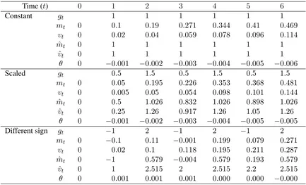
Time (t) 0 1 2 3 4 5 6

Constant gt 1 1 1 1 1 1

mt 0 0.1 0.19 0.271 0.344 0.41 0.469

vt 0 0.02 0.04 0.059 0.078 0.096 0.114

ˆ

mt 0 1 1 1 1 1 1

ˆ

vt 0 1 1 1 1 1 1

θ 0 −0.001 −0.002 −0.003 −0.004 −0.005 −0.006

Scaled gt 0.5 1.5 0.5 1.5 0.5 1.5

mt 0 0.05 0.195 0.226 0.353 0.368 0.481

vt 0 0.005 0.05 0.054 0.098 0.101 0.144

ˆ

mt 0 0.5 1.026 0.832 1.026 0.898 1.026

ˆ

vt 0 0.25 1.26 0.917 1.26 1.05 1.26

θ 0 −0.001 −0.002 −0.003 −0.004 −0.005 −0.005

Different sign gt −1 2 −1 2 −1 2

mt 0 −0.1 0.11 −0.001 0.199 0.079 0.271

vt 0 0.02 0.1 0.118 0.195 0.211 0.287

ˆ

mt 0 −1 0.579 −0.004 0.579 0.193 0.579

ˆ

vt 0 1 2.515 2 2.515 2.2 2.515

θ 0 0.001 0.001 0.001 0.000 0.000 −0.000

Table 2: The Adam optimizer slows down when gradients have larger variance even if they have the same average, in this case 1. When alternating between−1and2, Adam takes 6 steps before the parameter has the correct sign. Updates can even slow down if gradients point in the same direction but have different scales. The learning rate is α= 0.001.

In practice, gradients reported by different pro-cessors are usually not the same: they are noisy estimates of the true gradient. In Table 2, we show examples where noise causes Adam to slow down. Summing gradients smooths out some of the noise. Next, we examine the formal basis for this effect.

Formally, Adam estimates the full gradient with an exponentially decaying averagemtof gradients

gt.

mt←β1mt−1+ (1−β1)gt

whereβ1 is a decay hyperparameter. It also

com-putes a decaying averagevtof second moments

vt←β2vt−1+ (1−β2)g2t

whereβ2 is a separate decay hyperparameter. The

squaring g_t2 is taken element-wise. These esti-mates are biased because the decaying averages were initialized to zero. Adam corrects for the bias to obtain unbiased estimatesmˆtandˆvt.

ˆ

mt←mt/(1−β1t)

ˆ

vt←vt/(1−β2t)

These estimates are used to update parametersθ

θt←θt−1−α

ˆ mt

√

ˆ vt+

whereαis the learning rate hyperparameter and

prevents element-wise division by zero.

Replacing estimators in the update rule with statistics they estimate and ignoring the usually-minor

ˆ mt

√

ˆ vt+

≈ _pEgt

E(g2_t)

which expands following the variance identity

Egt

p

E(g2_t) =

Egt

p

V ar(gt) + (Egt)2

Dividing both the numerator and denominator by

|Egt|, we obtain

= p sign(Egt) V ar(gt)/(Egt)2+ 1

The termV ar(gt)/(Egt)2 is statistical efficiency, the square of coefficient of variation. In other words, Adam gives higher weight to gradients if historical samples have a lower coefficient of vari-ation. The coefficient of variation of a sum ofN

independent1samples decreases as1/√N. Hence sums (despite having less frequent updates) may

actually cause Adam to move faster because they have smaller coefficient of variation. An example appears in Table2: updating with 1 moves faster than individually applying -1 and 2.

4 Ablation Study

We conduct ablation experiments to investigate the poor performance in asynchronous Transformer training for the neural machine translation task.

4.1 Experiment Setup

Our experiments use systems for the WMT 2017 English to German news translation task. The Transformer is standard with six encoder and six decoder layers. The RNN model (Barone et al., 2017) is based on the winning WMT17 submission (Sennrich et al., 2017) with 8 layers. Both models use back-translated monolingual cor-pora (Sennrich et al.,2016a) and byte-pair encod-ing (Sennrich et al.,2016b).

We follow the rest of the hyperparameter set-tings on both Transformer and RNN models as suggested in the papers (Vaswani et al.,2017; Sen-nrich et al., 2017). Both models were trained on four GPUs with a dynamic batch size of 10 GB per GPU using the Marian toolkit ( Junczys-Dowmunt et al., 2018). Both models are trained for 8 epochs or until reaching five continuous vali-dations without loss improvement. Quality is mea-sured on newstest2016 using sacreBLEU (Post,

2018), preserving newstest2017 as test for later experiments. The Transformer’s learning rate is linearly warmed up for 16k updates. We apply an inverse square root learning rate decay follow-ingVaswani et al.(2017) for both models. All of these experiments use the Adam optimizer, which has shown to perform well on a variety of tasks (Kingma and Ba,2014) and was used in the origi-nal Transformer paper (Vaswani et al.,2017).

For subsequent experiments, we will use a learning rate of 0.0003 for Transformers and 0.0006 for RNNs. These were near the top in both asynchronous and synchronous settings (Table1).

4.2 Batch Size

We first explore the effect of batch size towards the model’s quality. We use dynamic batching, in which the toolkit fits as many sentences as it can into a fixed amount of memory (so e.g. more sen-tences will be in a batch if all of them are short). Hence batch sizes are denominated in memory

sizes. Our GPUs each have 10 GB available for batches which, on average, corresponds to 250 sentences.

With 4 GPUs, baseline synchronous SGD has an effective batch size of 40 GB, compared to 10 GB in asynchronous. We fill in the two missing scenarios: synchronous SGD with a total effec-tive batch size of 10 GB and asynchronous SGD with a batch size of 40 GB. Because GPU mem-ory is limited, we simulate a larger batch size in asynchronous SGD by locally accumulating gra-dients in each processor four times before sending the summed gradient to the parameter server (Ott et al.,2018;Bogoychev et al.,2018).

Models with a batch size of 40GB achieve better BLEUper update, compared with its 10GB vari-ant as shown in Figure1. However, synchronous SGD training still outperforms asynchronous SGD training, even with smaller batch size. From this experiment, we conclude that batch size is not the primary driver of poor performance of asyn-chronously trained Transformers, though it does have some lingering impact on final model qual-ity. For RNNs, batch size and distributed training algorithm had little impact beyond the early stages of training, continuing the theme that Transform-ers are more sensitive to noisy gradients.

4.3 Gradient Staleness

To study the impact of gradient staleness, we in-troduce staleness into synchronous SGD. Work-ers only pull the latest parameter once every U

updates, yielding an average staleness of (U−₂1). Since asynchronous SGD has average staleness3

with N = 4 GPUs, we set U = 7 to achieve the same average staleness of3. Additionally, we also tried a lower average staleness of 2 by set-ting U = 5. We also see the effect of doubling the learning rate so the parameter moves twice as far, hence introduces staleness in terms of model distance.

In order to focus on the impact of the staleness, we set the batch size to 40 GB total RAM con-sumption, be they 4 GPUs with 10 GB each in synchronous SGD or emulated 40 GB batches on each GPU in asynchronous SGD.

0 50 100 150 200 250 num updates x1000

0 10 20 30

validation BLEU

Convergence per-update

Trans + sync 40GB Trans + s nc 10GB Trans + sync 40GB Trans + s nc 10GB

(a) Convergence over updates in Transformer model with various batch sizes

0 20 40 60 80 100 num updates x1000

0 10 20 30

validation BLEU

Convergence per-update

RNN + sync 40 GB RNN + s nc 10 GB RNN + sync 40 GB RNN + s nc 10 GB

(b) Convergence over updates in RNN model with vari-ous batch sizes

Figure 1: The effect of batch sizes on convergence of Transformer and RNN models.

0 50 100 150 200 num updates x1000

0 10 20 30

validation BLEU

Convergence per-update (LR = 0.0003)

Trans + sync

Trans + sync + avg. staleness 2 Trans + sync + avg. staleness 3 Trans + sync

(a) Transformer model with lr = 0.0003

0 10 20 30 40 50 num updates x1000

0 10 20 30

validation BLEU

Convergence per-update (LR = 0.0006)

RNN + sync

RNN + sync + avg. staleness 2 RNN + sync + avg. staleness 3 RNN + sync

(b) RNN model with lr = 0.0006

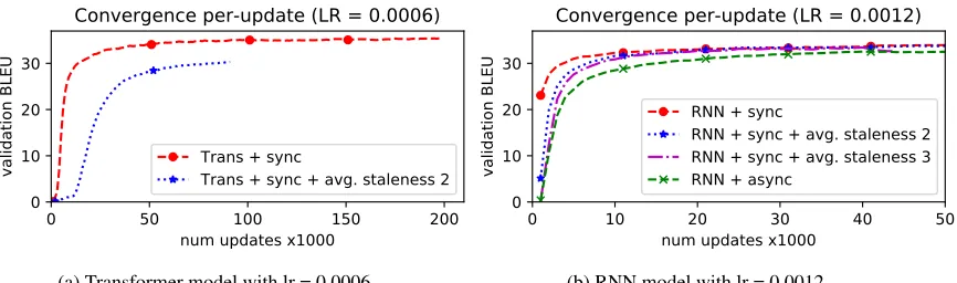
Figure 2: Artificial staleness in synchronous SGD compared to synchronous and asynchronous baselines, all with our usual learning rate for each model.

0 50 100 150 200 num updates x1000

0 10 20 30

validation BLEU

Convergence per-update (LR = 0.0006)

Trans + sync

Trans + sync + avg. staleness 2

(a) Transformer model with lr = 0.0006

0 10 20 30 40 50 num updates x1000

0 10 20 30

validation BLEU

Convergence per-update (LR = 0.0012)

RNN + sync

RNN + sync + avg. staleness 2 RNN + sync + avg. staleness 3 RNN + sync

(b) RNN model with lr = 0.0012

Figure 3: Artificial staleness in synchronous SGD with doubled learning rates. Transformers with learning rate 0.0006 and staleness 3 (synchronous and asynchronous) did not rise above 0.

RNNs to training conditions.

Results for Transformer worsen when we dou-ble the learning rate (Figure3). With staleness 3, the model stayed at 0 BLEU for both synchronous or asynchronous SGD, consistent with our earlier result (Table1).

We conclude that staleness is primary, but not wholly, responsible for the poor performance of asynchronous SGD in training Transformers. However, asynchronous SGD still underperforms synchronous SGD with artificial staleness of 3 and

5 Asynchronous Transformer Training

5.1 Accumulated Asynchronous SGD

Previous experiments have shown that increasing the batch size and reducing staleness improves the final quality of asynchronous training. Increasing the batch size can be achieved by accumulating gradients before updating. We experiment with variations on three ways to accumulate gradients:

Local Accumulation: Gradients can be accu-mulated locally in each processor before sending it to the parameter server (Ott et al.,2018; Bogoy-chev et al.,2018). This approach scales the effec-tive batch size and reduces communication costs as the workers communicate less often. However, this approach does not reduce staleness as the pa-rameter server updates immediately after receiv-ing a gradient. We experiment with accumulatreceiv-ing four gradients locally, resulting in 40 GB effective batch size.

Global Accumulation: Each processor sends the computed gradient to the parameter server nor-mally. However, the parameter server holds the gradient and only updates the model after it re-ceives multiple gradients (Dean et al.,2012;Lian et al., 2015). This approach scales the effective batch size. On top of that, it decreases staleness as the parameter server updates less often. However, it does not reduce communication costs. We ex-periment with accumulating four gradients glob-ally, resulting in 40 GB effective batch size and

0.75average staleness.

Combined Accumulation: Local and global accumulation can be combined to gain the bene-fits of both: reduced communication cost and re-duced average staleness. In this approach, gradi-ents are accumulated locally in each processor be-fore being sent. The parameter server also waits and accumulates gradients before running an opti-mizer. We accumulate two gradients both locally and globally. This yields in 40 GB effective batch size and1.5average staleness.

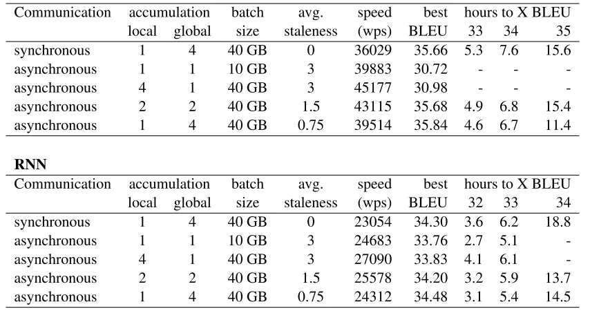
We tested the three gradient accumulation fla-vors on the English-to-German task with both Transformer and RNN models. Synchronous SGD also appears as a baseline. To compare results, we report best BLEU, raw training speed, and time needed to reach several BLEU checkpoints. Re-sults are shown in Table3.

Asynchronous SGD with global accumulation actually improves the final quality of the model over synchronous SGD, albeit not meaningfully.

This one change, accumulating every 4 gradients (the number of GPUs), restores quality in asyn-chronous methods. It also achieves the fastest time to reach near-convergence BLEU in both Trans-former and RNN.

While using local accumulation provides even faster raw speed, the model produces the worst quality among the other accumulation techniques. Asynchronous SGD with 4x local accumulation is essentially just ordinary asynchronous SGD with 4x larger batch size and 4x less update frequency. In particular, gradient staleness is still the same, therefore this does not help the convergence per-update.

Combined accumulation performs somewhat in the middle. It does not converge as fast as asyn-chronous SGD with full global accumulation but not as poor as asynchronous SGD with full local accumulation. Its speed is also in between, reflect-ing communication costs.

5.2 Generalization Across Learning Rates

Earlier in Table 1 we show that asynchronous Transformer learning is very sensitive towards the learning rate. In this experiment, we use an asyn-chronous SGD with global gradient accumulation to train English-to-German on different learning rates. We compare our result with vanilla syn-chronous and vanilla asynsyn-chronous SGD.

Our finding empirically show that asynchronous Transformer training while globally accumulat-ing the gradients is significantly more robust. As shown in Table 5, the model is now capable to learn on higher learning rate and yield compara-ble results compared to its synchronous variant.

5.3 Generalization Across Languages

To test whether our findings on English-to-German generalize, we train two more transla-tion systems using globally accumulated gradi-ents. Specifically, we train English to Finnish (EN

→FI) and English to Russian (EN→RU) models for the WMT 2018 task (Bojar et al., 2018). We validate our model on newstest2015 for EN→FI and newstest2017 for EN→RU. Then, we test our model on newstest2017 for EN → DE and new-stest2018 for both EN→ FI and EN→ RU. The same network structures and hyperparameters are used as before.

Transformer

Communication accumulation batch avg. speed best hours to X BLEU local global size staleness (wps) BLEU 33 34 35

synchronous 1 4 40 GB 0 36029 35.66 5.3 7.6 15.6

asynchronous 1 1 10 GB 3 39883 30.72 - -

-asynchronous 4 1 40 GB 3 45177 30.98 - -

-asynchronous 2 2 40 GB 1.5 43115 35.68 4.9 6.8 15.4

asynchronous 1 4 40 GB 0.75 39514 35.84 4.6 6.7 11.4

RNN

Communication accumulation batch avg. speed best hours to X BLEU local global size staleness (wps) BLEU 32 33 34

synchronous 1 4 40 GB 0 23054 34.30 3.6 6.2 18.8

asynchronous 1 1 10 GB 3 24683 33.76 2.7 5.1

-asynchronous 4 1 40 GB 3 27090 33.83 4.1 6.1

-asynchronous 2 2 40 GB 1.5 25578 34.20 3.2 5.9 13.7

asynchronous 1 4 40 GB 0.75 24312 34.48 3.1 5.4 14.5

Table 3: Quality and convergence of asynchronous SGD with accumulated gradients on English to German dataset. Dashes indicate that model never reach the target BLEU.

Model EN→DE EN→FI EN→RU

newstest 2016 2017 2017 2018 2015 2018

Trans. + synchronous SGD 35.66 28.81 18.47 14.03 29.31 25.49 Trans. + asynchronous SGD 30.72 24.68 11.63 8.73 21.12 17.78 Trans. + asynchronous SGD + 4x global accum. 35.84 28.66 18.47 13.78 29.12 25.25

RNN + synchronous SGD 34.30 27.43 16.94 12.75 26.96 23.11

RNN + asynchronous SGD 33.76 26.84 14.94 10.96 26.39 22.48

RNN. + asynchronous SGD + 4x global accum. 34.48 27.56 17.05 12.76 27.15 23.41

Table 4: The effect of global accumulation on translation quality for different language pairs on development and test set, measured with BLEU score.

Communication Sync. Async. Async

Learn Rate + 4x GA

0.0003 35.66 30.72 35.84

0.0006 35.42 0.00 35.81

0.0012 33.96 0.00 33.62

0.0024 29.35 0.00 1.20

Table 5: Performance of the asynchronous Transformer on English to German with 4x Global accumulations (GA) across different learning rates on development set measured with BLEU score.

larger batch size and a lower staleness in Trans-former massively improves the result, compared to basic asynchronous SGD (+6 BLEU on aver-age). The improvement is smaller in RNN experi-ment, but still substantial (+1 BLEU on average). We also have further confirmation that training

a Transformer model with normal asynchronous SGD is impractical.

6 Related Work

6.1 Gradient Summing

Several papers wait and sumP gradients from dif-ferent workers as a way to reduce staleness. In

Chen et al.(2016), gradients are accumulated from different processors, and whenever thePgradients have been pushed, other processors cancel their process and restart from the beginning. This is rel-atively wasteful since some computation is thrown out andP−1processors still idle for synchroniza-tion. Gupta et al.(2016) suggest that restarting is not necessary but processors still idle waiting for

con-tinually generate gradients without synchroniza-tion.

Another direction to overcome stale gradient is to reduce its effect towards the model update.

McMahan and Streeter(2014) dynamically adjust the learning rate depending on the staleness.Dutta et al. (2018) suggests completely ignoring stale gradient pushes.

6.2 Increasing Staleness

In the opposite direction, some work has added noise to gradients or increased staleness, typi-cally to cut computational costs. Recht et al.

(2011) propose a lock-free asynchronous gradient update. Lossy gradient compression by bit quanti-zation (Seide et al.,2014;Alistarh et al.,2017) or threshold based sparsification (Aji and Heafield,

2017;Lin et al.,2017) also introduce noisy gradi-ent updates. On top of that, these techniques store unsent gradients to be added into the next gradient, increasing staleness for small gradients.

Dean et al. (2012) mention that communica-tion overload can be reduced by reducing gradient pushes and parameter synchronization frequency. In McMahan et al. (2017), each processor inde-pendently updates its own local model and peri-odically synchronize the parameter by averaging across other processors. Ott et al.(2018) accumu-lates gradients locally, before sending it to the pa-rameter server. Bogoychev et al. (2018) also lo-cally accumulates the gradient, but also updates local parameters in between.

7 Conclusion

We evaluated the behavior of Transformer and RNN models under asynchronous training. We divide our analysis based on two main different aspects in asynchronous training: batch size and stale gradient. Our experimental results show that:

• In general, asynchronous training damages the final BLEU of the NMT model. However, we found that the damage with the Trans-former is significantly more severe. In ad-dition, asynchronous training also requires a smaller learning rate to perform well.

• With the same number of processors, asyn-chronous SGD has a smaller effective batch size. We empirically show that training un-der a larger batch size setting can slightly proves the convergence. However, the

im-provement is very minimal. The result in asynchronous Transformer model is subpar, even with a larger batch size.

• Stale gradients play a bigger role in the training performance of asynchronous Trans-former. We have shown that the Transformer model’s performed poorly by adding a syn-thetic stale gradient.

Based on these findings, we suggest applying a modification in asynchronous training by accumu-lating a few gradients (for example for the number of processors) in the server before applying an up-date. This approach increases the batch size while also reducing the average staleness. We empiri-cally show that this approach combine the high quality training of synchronous SGD and high training speed of asynchronous SGD.

Future works should extend those experiments to different hyper-parameter configurations. One direction is to investigate wether vanilla asyn-chronous Trasnformer can be trained under dif-ferent optimizers. Another direction is to exper-iment with more workers where gradients in asyn-chronous SGD are more stale.

8 Acknowledgements

Alham Fikri Aji is funded by the Indone-sia Endowment Fund for Education scholarship scheme. This work was performed using re-sources provided by the Cambridge Service for Data Driven Discovery (CSD3) operated by the University of Cambridge Research Computing Service (http://www.csd3.cam.ac.uk/), provided by Dell EMC and Intel using Tier-2 fund-ing from the Engineerfund-ing and Physical Sciences Research Council (capital grant EP/P020259/1), and DiRAC funding from the Science and Tech-nology Facilities Council (www.dirac.ac. uk).

References

Alham Fikri Aji and Kenneth Heafield. 2017. Sparse communication for distributed gradient descent. In

Proceedings of the 2017 Conference on Empirical

Methods in Natural Language Processing, pages

440–445.

Dan Alistarh, Demjan Grubic, Jerry Li, Ryota Tomioka, and Milan Vojnovic. 2017. Qsgd: Communication-efficient sgd via gradient quantiza-tion and encoding. InAdvances in Neural

Antonio Valerio Miceli Barone, Jindˇrich Helcl, Rico Sennrich, Barry Haddow, and Alexandra Birch. 2017. Deep architectures for neural machine trans-lation. InProceedings of the Second Conference on

Machine Translation, pages 99–107.

Nikolay Bogoychev, Kenneth Heafield, Alham Fikri Aji, and Marcin Junczys-Dowmunt. 2018. Accel-erating asynchronous stochastic gradient descent for neural machine translation. In Proceedings of the 2018 Conference on Empirical Methods in Natural

Language Processing, pages 2991–2996.

Ondej Bojar, Christian Federmann, Mark Fishel, Yvette Graham, Barry Haddow, Matthias Huck, Philipp Koehn, and Christof Monz. 2018. Find-ings of the 2018 conference on machine translation (wmt18). In Proceedings of the Third Conference on Machine Translation (WMT), Volume 2: Shared

Task Papers, pages 272–307. Association for

Com-putational Linguistics.

Jianmin Chen, Xinghao Pan, Rajat Monga, Samy Bengio, and Rafal Jozefowicz. 2016. Revisit-ing distributed synchronous sgd. arXiv preprint

arXiv:1604.00981.

Mia Xu Chen, Orhan Firat, Ankur Bapna, Melvin Johnson, Wolfgang Macherey, George Foster, Llion Jones, Niki Parmar, Mike Schuster, Zhifeng Chen, et al. 2018. The best of both worlds: Combining re-cent advances in neural machine translation. arXiv preprint arXiv:1804.09849.

Jeffrey Dean, Greg Corrado, Rajat Monga, Kai Chen, Matthieu Devin, Mark Mao, Andrew Senior, Paul Tucker, Ke Yang, Quoc V Le, et al. 2012. Large scale distributed deep networks. In Advances in neural information processing systems, pages 1223– 1231.

Sanghamitra Dutta, Gauri Joshi, Soumyadip Ghosh, Parijat Dube, and Priya Nagpurkar. 2018. Slow and stale gradients can win the race: Error-runtime trade-offs in distributed sgd. arXiv preprint

arXiv:1803.01113.

Suyog Gupta, Wei Zhang, and Fei Wang. 2016. Model accuracy and runtime tradeoff in distributed deep learning: A systematic study. In 2016 IEEE 16th

International Conference on Data Mining (ICDM),

pages 171–180. IEEE.

Marcin Junczys-Dowmunt, Roman Grundkiewicz, Tomasz Dwojak, Hieu Hoang, Kenneth Heafield, Tom Neckermann, Frank Seide, Ulrich Germann, Alham Fikri Aji, Nikolay Bogoychev, Andr´e F. T. Martins, and Alexandra Birch. 2018. Marian: Fast neural machine translation in C++. InProceedings

of ACL 2018, System Demonstrations, pages 116–

121, Melbourne, Australia. Association for Compu-tational Linguistics.

Diederik P Kingma and Jimmy Ba. 2014. Adam: A method for stochastic optimization. arXiv preprint arXiv:1412.6980.

Xiangru Lian, Yijun Huang, Yuncheng Li, and Ji Liu. 2015. Asynchronous parallel stochastic gradient for nonconvex optimization. InAdvances in Neural

In-formation Processing Systems, pages 2737–2745.

Yujun Lin, Song Han, Huizi Mao, Yu Wang, and William J Dally. 2017. Deep gradient compression: Reducing the communication bandwidth for dis-tributed training. arXiv preprint arXiv:1712.01887. Brendan McMahan, Eider Moore, Daniel Ramage,

Seth Hampson, and Blaise Aguera y Arcas. 2017. Communication-efficient learning of deep networks from decentralized data. In Artificial Intelligence and Statistics, pages 1273–1282.

Brendan McMahan and Matthew Streeter. 2014. Delay-tolerant algorithms for asynchronous dis-tributed online learning. InAdvances in Neural

In-formation Processing Systems, pages 2915–2923.

Myle Ott, Sergey Edunov, David Grangier, and Michael Auli. 2018. Scaling neural machine trans-lation. In Proceedings of the Third Conference on

Machine Translation: Research Papers, pages 1–9.

Martin Popel and Ondˇrej Bojar. 2018. Training tips for the transformer model. The Prague Bulletin of Mathematical Linguistics, 110(1):43–70.

Matt Post. 2018. A call for clarity in reporting bleu scores. InProceedings of the Third Conference on

Machine Translation: Research Papers, pages 186–

191.

Benjamin Recht, Christopher Re, Stephen Wright, and Feng Niu. 2011. Hogwild: A lock-free approach to parallelizing stochastic gradient descent. In

Ad-vances in neural information processing systems,

pages 693–701.

Frank Seide, Hao Fu, Jasha Droppo, Gang Li, and Dong Yu. 2014. 1-bit stochastic gradient descent and its application to data-parallel distributed train-ing of speech dnns. InFifteenth Annual Conference of the International Speech Communication Associ-ation.

Rico Sennrich, Alexandra Birch, Anna Currey, Ulrich Germann, Barry Haddow, Kenneth Heafield, An-tonio Valerio Miceli Barone, and Philip Williams. 2017. The University of Edinburgh’s neural mt sys-tems for WMT17. In Proceedings of the Second

Conference on Machine Translation, pages 389–

399.

Rico Sennrich, Barry Haddow, and Alexandra Birch. 2016b. Neural machine translation of rare words with subword units. InProceedings of the 54th An-nual Meeting of the Association for Computational Linguistics, pages 1715–1725.

Samuel L Smith, Pieter-Jan Kindermans, Chris Ying, and Quoc V Le. 2017. Don’t decay the learn-ing rate, increase the batch size. arXiv preprint

arXiv:1711.00489.

Anand Srinivasan, Ajay Jain, and Parnian Barekatain. 2018. An analysis of the delayed gradients problem in asynchronous SGD.

Ashish Vaswani, Noam Shazeer, Niki Parmar, Jakob Uszkoreit, Llion Jones, Aidan N Gomez, Łukasz Kaiser, and Illia Polosukhin. 2017. Attention is all you need. InAdvances in Neural Information Pro-cessing Systems, pages 5998–6008.

Chong Wang, Xi Chen, Alexander J Smola, and Eric P Xing. 2013. Variance reduction for stochastic gra-dient optimization. InAdvances in Neural Informa-tion Processing Systems, pages 181–189.