Graded Word Sense Assignment
Katrin Erk
University of Texas at Austin
Diana McCarthy University of Sussex
Abstract
Word sense disambiguation is typically phrased as the task of labeling a word in context with the best-fitting sense from a sense inventory such as WordNet. While questions have often been raised over the choice of sense inventory, computational linguists have readily accepted the best-fitting sense methodology despite the fact that the case for discrete sense bound-aries is widely disputed by lexical seman-tics researchers. This paper studiesgraded word sense assignment, based on a recent dataset of graded word sense annotation.
1 Introduction
The task of automatically characterizing word meaning in text is typically modeled as word sense disambiguation (WSD): given a list of senses for
target lemmaw, the task is to pick the best-fitting sense for a given occurrence of w. The list of senses is usually taken from an online dictionary or thesaurus. However, clear cut sense boundaries are sometimes hard to define, and the meaning of words depends strongly on the context in which they are used (Cruse, 2000; Hanks, 2000). Some researchers in lexical semantics have suggested that word meanings lie on a continuum between i) clear cut cases of ambiguity and ii) vagueness where clear cut boundaries do not hold (Tuggy, 1993). Certainly, it seems that a more complex representation of word sense is needed with a softer, graded representation of meaning rather than a fixed listing of senses (Cruse, 2000).
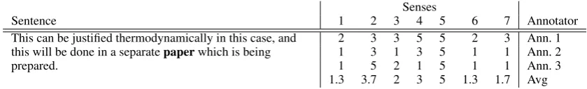
A recent annotation study ((Erk et al., 2009), hereafter GWS) marked a target word in context with graded ratings (on a scale of 1-5) on senses from WordNet (Fellbaum, 1998). Table 1 shows an example of a sentence with the target word in bold, and with the annotator judgments given
to each sense. The study found that annotators made ample use of the intermediate ratings on the scale, and often gave high ratings to more than one WordNet sense for the same occurrence. It was found that the annotator ratings could not easily be transformed to categorial judgments by making more coarse-grained senses. If human word sense judgments are best viewed as graded, it makes sense to explore models of word sense that can predict graded sense assignments.
In this paper we look at the issue of graded ap-plicability of word sense from the point of view of automatic graded word sense assignment, us-ing theGWSgraded word sense dataset. We make
three primary contributions. Firstly, we propose evaluation metrics that can be used on graded word sense judgments. Some of these metrics, like Spearman’s ρ, have been used previously (Mc-Carthy et al., 2003; Mitchell and Lapata, 2008), but we also introduce new metrics based on the traditional precision and recall. Secondly, we in-vestigate how two classes of models perform on the task of graded word sense assignment: on the one hand classical WSDmodels, on the other
hand prototype-based vector space models that can be viewed as simple one-class classifiers. We study supervised models, training on traditional
WSD data and evaluating against a graded scale.
Thirdly, the evaluation metrics we use also pro-vides a novel analysis of annotator performance on theGWSdataset.
2 Related Work
WSDhas to date been a task where word senses are
viewed as having clear cut boundaries. However, there are indications that word meanings do not behave in this way (Kilgarriff, 2006). Researchers in the field ofWSDhave acknowledged these
prob-lems but have used existing lexical resources in the hope that useful applications can be built with them. However, there is no consensus on which
Senses
Sentence 1 2 3 4 5 6 7 Annotator
This can be justified thermodynamically in this case, and this will be done in a separatepaperwhich is being prepared.
2 3 3 5 5 2 3 Ann. 1
1 3 1 3 5 1 1 Ann. 2
1 5 2 1 5 1 1 Ann. 3
[image:2.595.88.508.62.126.2]1.3 3.7 2 3 5 1.3 1.7 Avg
Table 1: A sample annotation in theGWSexperiment. The senses are: 1 material from cellulose 2 report
3 publication 4 medium for writing 5 scientific 6 publishing firm 7 physical object
inventory is suitable for which application, other than cross-lingual applications where the inven-tory can be determined from parallel data (Carpuat and Wu, 2007; Chan et al., 2007). For monolin-gual applications however it is less clear whether current state-of-the-art WSD systems for tagging
text with dictionary senses are able to have an im-pact on applications.
One way of addressing the problem of low inter-annotator agreement and system performance is to create an inventory that is coarse-grained enough for humans and computers to do the job reli-ably (Ide and Wilks, 2006; Hovy et al., 2006; Palmer et al., 2007). Such coarse-grained invento-ries can be produced manually from scratch (Hovy et al., 2006) or by automatically relating (Mc-Carthy, 2006) or clustering (Navigli, 2006; Nav-igli et al., 2007) existing word senses. While the reduction in polysemy makes the task easier, we do not know which are the right distinctions to re-tain. In fact, fine-grained distinctions may be more useful than coarse-grained ones for some applica-tions (Stokoe, 2005). Furthermore, Hanks (2000) goes further and argues that while the ability to distinguish coarse-grained senses is indeed desir-able, subtler and more complex representations of word meaning are necessary for text understand-ing.
In this paper, instead of focusing on issues of granularity we try to predict graded judgments of word sense applicability, using a recent dataset with graded annotation (Erk et al., 2009). Our hope is that models which can mimic graded hu-man judgments on the same task should better re-flect the underlying phenomena of word mean-ing compared to a system that focuses on mak-ing clear cut distinctions. Also, we hope that such models might prove more useful in applications. There is one existing study of graded sense as-signment (Ramakrishnan et al., 2004). It tries to estimate a probability distribution over senses by converting all of WordNet into a huge Bayesian Network, and reports improvements in a Question
Answering task. However, it does not test its pre-diction against human annotator data.
We concentrate on supervised models in this paper since they generally perform better than their unsupervised or knowledge-based counter-parts (Navigli, 2009). We compare them against a baseline model which simply uses the train-ing data to obtain a probability distribution over senses regardless of context, since marginal distri-butions are highly skewed making a prior distribu-tion very informative (Chan and Ng, 2005; Lapata and Brew, 2004).
Along with standard WSD models, we
evalu-ate vector space models that use the training data to locate a word sense in semantic space. Word sense and vector space models have been related in two ways. On the one hand, vector space models have been used for inducing word senses (Sch¨utze, 1998; Pantel and Lin, 2002). The different mean-ings of a word are obtained by clustering vectors. The clusters must then be mapped to an inven-tory if a standard WSD dataset is used for
eval-uation. In contrast, we use sense tagged train-ing data with the aim of buildtrain-ing models of given word senses, rather than clustering occurrences into word senses. The second way in which word sense and vector space models have been related is to assign disambiguated feature vectors to Word-Net concepts (Pantel, 2005; Patwardhan and Ped-ersen, 2006). However those works do not use sense-tagged data and are not aimed atWSD, rather
the applications are to insert new concepts into an ontology and to measure the relatedness of con-cepts.
lemma # # training (PoS) senses SemCor SE-3
add (v) 6 171 238
argument (n) 7 14 195
ask (v) 7 386 236
different (a) 5 106 73
important (a) 5 125 11
interest (n) 7 111 160
paper (n) 7 46 207
win (v) 4 88 53
[image:3.595.99.263.66.183.2]total training sentences 1047 1173
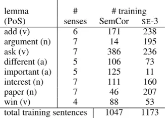
Table 2: Lemmas used in this study
with various sense-tagged datasets (e.g. (Miller et al., 1993; Mihalcea et al., 2004)) for comparison.
3 Data
In this paper, we use a subset of the GWS
dataset (Erk et al., 2009) where three annotators supplied ordinal judgments of the applicability of WordNet (v3.0) senses on a 5 point scale: 1 –
completely different, 2 –mostly different, 3 – sim-ilar, 4 – very similar and 5 – identical. Table 1 shows a sample annotation. The sentences that we use from the GWSdataset were originally
ex-tracted from the EnglishSENSEVAL-3 lexical
sam-ple task (Mihalcea et al., 2004) (hereafter SE-3)
and SemCor (Miller et al., 1993). 1 For 8
lem-mas, 25 sentences were randomly sampled from SemCor and 25 randomly sampled fromSE-3,
giv-ing a total of 50 sentences per lemma. The lem-mas, their PoS and number of senses from Word-Net are shown in table 2.
The annotation study found that annotators made ample use of the intermediate levels of ap-plicability (2-4), and they often gave positive rat-ings (3-5) to more than one sense for a single oc-currence. The example in Table 1 is one such case. An analysis of the annotator ratings found that they could not easily be explained in catego-rial terms by making more coarse-grained senses because senses that were not positively correlated often had high ratings for the same instance.
The GWSdataset contains a sequence of
judg-ments for each occurrence of a target word in a sentence context: one judgment for each Word-Net sense of the target word. To obtain a sin-gle judgment for each sense in each sentence we use the average judgment from the three annota-tors. As models typically assign values between
1TheGWSdata also contains data from the English Lex-ical Substitution Task (McCarthy and Navigli, 2007) but we do not use that portion of the data for these experiments.
0 and 1, we normalize the annotator judgments from theGWSdataset to fall into the same range by
using normalized judgment = (judgment− 1.0)/4.0. This maps an original judgment of 5 to a normalized judgment of 1.0, it maps an original 1 to 0.0, and intermediate judgments are mapped accordingly.
As theGWSdataset is too small to accommodate
both training and testing of a supervised model, we use all the data fromGWSfor testing our models,
and train our models on traditional word sense an-notation data. We use as training data all sentences from SemCor and the training portion ofSE-3 that
are not included inGWS. The quantity of training
data available is shown in the last two columns of table 2.
4 Evaluating Graded Word Sense Assignment
This section discusses measures for evaluating system performance for the case where gold judg-ments are graded rather than categorial.
Correlation. The standard method for compar-ing a list of graded gold judgments to a list of graded predicted judgments is by testing for corre-lation. In our case, as we cannot assume a normal distribution of the judgments, a non-parametric test such as Spearman’s ρ will be appropriate. Spearman’sρuses the formula of Pearson’s coef-ficient, defined as
ρ(X, Y) = cov(X, Yσ )
XσY
Pearson’s coefficient computes the correlation of two random variables X and Y as their covari-ance divided by the product of their standard devi-ations. In the computation of Spearman’sρ, values are transformed to rankings before the formula is applied. 2 As Spearman’s ρ compares the
rank-ings of two sets of judgments, it abstracts from the absolute values of the judgments. It is useful to have a measure that abstracts from absolute values of judgments and magnitude of difference because theGWSdataset contains annotator judgments on
a fixed scale, and it is quite possible that human judges will differ in how they use such a scale.
Each judgment in the gold-standard can be represented as a 4-tuple hlemma, sense no, sen-tence no, gold judgmenti. For example, hadd.v,
1, 1, 0.8iis the first sentence for targetadd.v, first WordNet sense, with a (normalized) judgment of 0.8. Likewise, each prediction by the model can be represented as a 4-tuplehlemma, sense no, sen-tence no, predicted judgmenti. We writeGfor the set of gold tuples,Afor the set of assigned tuples,
L for the set of lemmas, S` for the set of sense
numbers that exist for lemma`, andT for the set of sentence numbers (there are 50 sentences for each lemma). We writeG|lemma=`for the gold set
restricted to those tuples with lemma`, and anal-ogously for other set restrictions and forA. There are several possibilities for measuring correlation:
by lemma: for each lemma` ∈ L, compute cor-relation betweenG|lemma=`andA|lemma=`
by lemma+sense: for each lemma ` and each sense number i ∈ S`, compute
cor-relation between G|lemma=`,senseno=i and
A|lemma=`,senseno=i
by lemma+sentence: for each lemma`and sen-tence number t ∈ T, compute cor-relation between G|lemma=`,sentence=t and
A|lemma=`,sentence=t
Comparison by lemma tests for the consis-tent use of judgments for the same target lemma. A comparison by lemma+sense ranks all occur-rences of the same target lemma by how strongly they evoke a given word sense. A comparison by lemma+sentence ranks different senses by how strongly they apply to a given target lemma oc-currence. In reporting correlation by lemma (by lemma+sense, by lemma+sentence), we average over all lemmas (lemma+sense, lemma+sentence combinations), and we report the percentage of lemmas (combinations) for which the correlation was significant. We report averaged correlation by lemma rather than one overall correlation over all judgments in order not to give more weight to lem-mas with more senses.
Divergence. Another possibility for measuring the performance of a graded sense assignment model is to use Jensen/Shannon divergence (J/S), which is a symmetric version of Kullback/Leibler divergence. Given two probability distributions
p, q, the Kullback/Leibler divergence ofq fromp
is
D(p||q) =X
x
p(x) logp(x)q(x)
and their J/S is
JS(p, q) = 12 D(p||p+2 q) +D(q||p+2 q)
We will use J/S for an evaluation by
lemma+sentence: for each lemma ` ∈ L
and sentence number t ∈ T, we normalize
G|lemma=`,sentence=t, the set of judgments for
senses of`int, by the sum of sense judgments for
`andt. We do the same forA|lemma=`,sentence=t.
Then we compute J/S. In doing so, we are not trying to interpret G|lemma=`,sentence=t as some
kind of probability distribution over senses, rather we use J/S as a measure that abstracts from absolute judgments but not from the magnitude of differences between judgments.
Precision and Recall. We have discussed a measure that abstracts from both absolute judg-ments and magnitude of differences (Spearman’s
ρ), and a measure that abstracts from absolute judgments but not the magnitude of differences (J/S). What is still missing is a measure that tests to what degree a model conforms to the absolute judgments given by the human annotators.
To obtain a measure for performance in predict-ing absolute gold judgments, we generalize preci-sion and recall. In the categorial case, precipreci-sion is defined as P = true positivestrue positives+false positives, true pos-itives divided by system-assigned pospos-itives, and recall is R = true positivestrue positives+false negatives, true posi-tives divided by gold posiposi-tives. Writing gold`,i,t for the judgment j associated with lemma ` and sense numberifor sentencetin the gold data (i.e.,
h`, i, t, ji ∈G), and analogously assigned`,i,t, we extend precision and recall to the graded case as follows:
P`=
P
i∈S`,tP∈T min(gold`,i,t,assigned`,i,t)
i∈S`,t∈T assigned`,i,t
and
R`=
P
i∈S`,t∈TPmin(gold`,i,t,assigned`,i,t)
i∈S`,t∈Tgold`,i,t
where`is a lemma. We compute precision and re-call by lemma, then macro-average them in order not to give more weight to lemmas that have more senses. The formula for F-score as the harmonic mean of precision and recall remains unchanged:
F = 2P R/(P+R).
Cx/2 until, IN, soft, JJ, remaining, VBG, ingredient, NNS
Cx/50 for, IN, sweet-sour, NN, sauce, NN, . . . , to, TO, a, DT, boil, NN
Ch OA, OA/ingredient/NNS
Table 3: Sample features foradd in BNC occur-renceFor sweet-sour sauce, cook onion in oil un-til soft. Add remaining ingredients and bring to a boil. Cx/2 (Cx/50): context of size 2 (size 50) either side of the target. Ch: children of target.
and recall, which can be seen as follows. Graded sense assignment is represented by assigning each sense a score between 0.0 and 1.0. The categorial case can be represented in the same way, the dif-ference being that one single sense will receive a score of 1.0 while all other senses get a score of 0.0. With this representation for categorial sense assignment, consider a fixed tokent of lemma`. P
i∈S`min(assigned`,i,t,gold`,i,t)will be 1 if the
assigned sense is the gold sense, and 0 otherwise.
5 Models for Graded Word Sense Assignment
In this section we discuss the computational mod-els for graded word sense that are tested in this paper.
Single-best-senseWSD. The first model that we test is a standardWSDmodel that assigns, to each
test occurrence of a target word, a single best-fitting word sense. The system thus attributes a confidence score of 1 to the assigned sense and a confidence score of 0 for all other senses for that sentence. We refer to it asWSD/single. The model uses standard features: lemma and part of speech in a narrow context window (2 words either side) and a wide context window (50 words either side), as well as dependency labels leading to parent, children, and siblings of the target word, and lem-mas and part of speech of parent, child, and sibling nodes. Table 3 shows sample model features for an occurrence ofaddin the British National Corpus (BNC) (Leech, 1992). The model uses a maxi-mum entropy learner3, training one binary
classi-fier per sense. (With n-ary classiclassi-fiers, the model’s performance is slightly worse.) The model is thus not highly optimized, but fairly standard.
WSDconfidence level as judgment. Our second model is the sameWSD system as above, but we
3http://maxent.sourceforge.net/
use it to predict a judgment for each sense of a target occurrence, taking the confidence level re-turned by each sense-specific binary classifier as the predicted judgment. We refer to this model as
WSD/conf.
Word senses as points in semantic space. The results of theGWSannotation study raise the
ques-tion of how word senses are best conceptualized, given that annotators assigned graded judgments of applicability of word senses, and given that they often combined high judgments for multiple word senses. One way of modeling these findings is to view word senses as prototypes, where some uses of a word will be typical examples of a given sense, for some uses the sense will clearly not ap-ply, and to some uses the sense will be borderline applicable.
We use a very simple model of word senses as prototypes, representing them as points in a se-mantic space. Graded sense applicability judg-ments can then be modeled using vector similarity. The dimensions of the vector space are the features of the WSD system above (including dimensions
likeCx2/until,Cx2/IN,Ch/OA/ingredient/NNSfor the example in Table 3), and the coordinates are raw feature counts. We compute a single vector for each sense s, the centroid of all training oc-currences that have been labeled withs. The pre-dicted judgment for a test sentence and sense s
is then the similarity of the sentence’s vector to the centroid vector fors, computed usingcosine. We call this modelPrototype. Like instance-based learners (Daelemans and den Bosch, 2005), the
Prototype model measures the distance between feature vectors in space. Unlike instance-based learners, it only uses data from a single category for training.
As it is to be expected that the vectors in this space will be very sparse, we also test a variant of thePrototypemodel with Sch¨utze-style second-order vectors (Sch¨utze, 1998), calledPrototype/2. Given a (first-order) feature vector, we compute a second-order vector as the centroid of vectors for all lemma features (omitting stopwords) in the first-order vector. For the feature vector in Table 3, this is the centroid of vectors sweet-sour~ , sauce~ , . . . ,boil~ . We compute the vectorssweet-sour~ etc. as dependency vectors (Pad´o and Lapata, 2007)4
over a Minipar parse (Lin, 1993) of the BNC.
4We use theDVpackage,http://www.nlpado.de/
We transform raw co-occurrence counts in the BNC-based vectors using pointwise mutual in-formation (PMI), a common transin-formation func-tion (Mitchell and Lapata, 2008).5
Another way of motivating the use of vector space models of word sense is by noting that we are trying to predict graded sense assignment by training on traditional word sense annotated data, where each target word occurrence is typically marked with a single word sense. Traditional word sense annotation, when used to predictGWS
judg-ments, will contain spurious negative data: sup-pose a human annotator is annotating an occur-rence of target wordtand views sensess1,s2and
s3as somewhat applicable, with senses1applying most clearly. Then if the annotation guidelines ask for the best-fitting sense, the annotator should only assign s1. The occurrence is recorded as having senses1, but not sensess2ands3. This, then, con-stitutes spurious negative data for sensess2ands3. The simple vector space model of word sense that we use implements a radical solution to this prob-lem of spurious negative data: it only uses positive data for a single sense, thus forgoing competition between categories. It is to be expected that not using competition between categories will hurt the vector space model’s performance, but this design gives us the chance to compare two model classes that use opposing strategies with respect to spuri-ous negative data: theWSDmodels fully trust the
negative data, while the vector space models ig-nore it.
6 Experiments
This section reports on experiments for the task of graded word sense assignment. As data, we use theGWS dataset described in Sec. 3. We test
the models discussed in Sec. 5, evaluating with the methods described in Sec. 4.
To put the models’ performance into perspec-tive, we first consider the human performance on the task, shown in Table 4. The first three lines of the table show the performance of each annota-tor evaluated against the average of the other two. The fourth line averages over the previous three lines to provide an average human ceiling for the task. In the correlation of rankings by lemma, cor-relation is statistically significant for all lemmas at
5We also tested PMI transformation for the first-order vec-tors, but will not report the results here as they were worse across the board than without PMI.
p≤0.01. For correlation by lemma+sense and by lemma+sentence, the percentage of pairs with sig-nificant correlation is lower: 73.6 of lemma/sense pairs and 29.0 of lemma/sentence pairs reach sig-nificance at p ≤ 0.05. For p ≤ 0.01, the per-centage is 58.3 and 12.2, respectively. The higher
ρ but lower proportion of significant values for lemma+sentence pairs compared to lemma+sense is due to the fact that there are far fewer dat-apoints (sample size) for each calculation of ρ
(#senses for lemma+sentence vs 50 sentences for lemma+sense).
At 0.131, J/S for Annotator 1 is considerably lower than for Annotators 2 and 3. 6 In terms
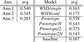
of precision and recall, Annotator 1 again differs from the other two. At 87.5, her recall is higher than her precision (50.6), while the other annota-tors have considerably higher precision (75.5 and 82.4) than recall (62.4 and 52.3). This indicates that Annotator 1 tended to assign higher ratings throughout, an impression that is confirmed by Ta-ble 6. The left two columns show average rat-ings for each annotator over all senses of all to-kens (normalized to values between 0.0 and 1.0 as described in Sec. 3). The three annotators differ widely in their average ratings, which range from 0.285 for Ann.3 to 0.540 for Ann.1.
Standard WSD. We tested the performance of the WSD/single model on a standard WSD task,
using the same training and testing data as in our subsequent experiments, as described in sec-tion 3.7 The model’s accuracy when trained and
tested on SemCor was A=77.0%, with a most fre-quent sense baseline of 63.5%. When trained and tested onSE-3, the model achieved A=53.0%
against a baseline of 44.0%. When trained and tested on SemCor plusSE-3, the model reached an
accuracy 58.2%, with a baseline of 56.0%. So on the combined dataset, the baseline is the average of the baselines on the individual datasets, while the model’s performance falls below the average performance on the individual datasets.
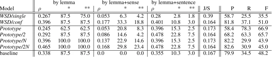
WSD models for graded sense assignment. Table 5 shows the performance of different mod-els in the task of graded word sense assignment. The first line in Table 5 lists results for the maxi-mum entropy model when used to assign a single best sense. The second line lists the results for
6Low J/S implies a closer agreement between two sets of judgments.
7Note that this constitutes less training data than in the
by lemma by lemma+sense by lemma+sentence
Ann ρ * ** ρ * ** ρ * ** J/S P R F
[image:7.595.87.511.63.126.2]Ann.1 0.517 100.0 100.0 0.407 75.0 58.3 0.482 27.3 11.5 0.131 50.6 87.5 64.1 Ann.2 0.587 100.0 100.0 0.403 68.8 58.3 0.612 38.1 17.2 0.153 75.5 62.4 68.3 Ann.3 0.528 100.0 100.0 0.41 77.1 58.3 0.51 21.8 7.8 0.165 82.4 52.3 64.0 Avg 0.544 100.0 100.0 0.407 73.6 58.3 0.535 29.0 12.2 0.149 69.5 67.4 65.5
Table 4: Human ceiling: one annotator vs. average of the other two annotators. ∗, ∗∗: percentage significant atp≤0.05,p≤0.01. Avg: average annotator performance
by lemma by lemma+sense by lemma+sentence
Model ρ * ** ρ * ** ρ * ** J/S P R F
WSD/single 0.267 87.5 75.0 0.053 6.3 4.2 0.28 2.8 1.8 0.39 58.7 25.5 35.5 WSD/conf 0.396 87.5 87.5 0.177 33.3 18.8 0.401 10.8 3.0 0.164 81.8 37.1 51.0 Prototype 0.245 62.5 62.5 0.053 20.8 8.3 0.396 15.3 2.5 0.173 58.4 78.3 66.9 Prototype/2 0.292 87.5 87.5 0.086 14.6 4.2 0.478 22.8 7.5 0.164 68.2 63.3 65.7 Prototype/N 0.396 100.0 100.0 0.137 22.9 14.6 0.396 15.3 2.5 0.173 82.2 29.9 43.9 Prototype/2N 0.465 100.0 100.0 0.168 29.8 23.4 0.478 22.8 7.5 0.164 82.6 30.9 45.0 baseline 0.338 87.5 87.5 0.0 0.0 0.0 0.355 10.3 3.0 0.167 79.9 34.5 48.2
Table 5: Evaluation: computational models, and baseline. ∗, ∗∗: percentage significant at p ≤ 0.05,
p≤0.01
the same maximum entropy model when classifier confidence is used as predicted judgment. The last line shows the baseline, an adaptation of the most frequent sense baseline to the graded case. For this baseline, we computed the relative frequency of each sense in the training corpus and used this relative frequency as the prediction for each test sentence and sense combination. TheWSD/single
model remains below the baseline in all evalua-tions except correlation by lemma+sense, where no rank-based correlation could be computed for the baseline because it always assigns the same judgment for a given sense. WSD/conf shows a performance slightly above the baseline in all eval-uation measures. Table 6 lists average ratings, av-eraged over all lemmas, senses, and occurrences, for each model in the two right-hand columns.
Prototype models. Lines 3-6 in Tables 5 and 6 show results forPrototypevariants. While each
Prototype and Prototype/2 model only sees pos-itive data annotated for a single sense, the vari-ants with/N(lines 5 and 6) make very limited use of information coming from all senses of a given lemma. They normalize judgments for each sen-tence, with
assignednorm`,i,t = P assigned`,i,t
j∈S`assigned`,j,t
Line 3 evaluates thePrototypemodel with first-order vectors. Its correlation with the gold data is somewhat lower than that ofWSD/conf in almost all cases.8 ThePrototypemodel deviates strongly 8The reason why the average ρ for correlation by
from bothWSD/conf and baseline in having a very good recall, at 78.3, with lower precision at 58.4, for an overall F-score that is 16 points higher than that ofWSD/conf. BothPrototypeandPrototype/2
have average ratings (Table 6) far above those of the WSD models and of the /N variants. The
second-order vector model Prototype/2 has rela-tively low correlation by lemma+sense, while cor-relation by lemma+sentence shows the best per-formance of all models (along withPrototype/2N). Its correlation by lemma+sentence is similar to the lowest correlation by lemma+sentence achieved by a human annotator. In terms of J/S, this model also shows the best performance along with
WSD/conf and Prototype/2N. Both /N variants achieve very high correlation by lemma. Corre-lation by lemma+sense for the /N models is be-tween those ofPrototypeandWSD/conf. The cor-relation by lemma+sentence is the same with or without normalization, as normalization does not change the ranking of senses of an individual sen-tence. WhilePrototypehas higher recall than pre-cision, normalization turns it into a model with even higher precision than WSD/conf but even lower recall.
Discussion
[image:7.595.77.521.172.265.2]Ann. avg Model avg Ann.1 0.540 WSD/single 0.163 Ann.2 0.345 WSD/conf 0.173 Ann.3 0.285 Prototype 0.558 Prototype/N 0.143 Prototype/2 0.375 Prototype/2N 0.143 baseline 0.167
Table 6: Average judgment for individual annota-tors (transformed) and average rating for models
(2009). Human annotators show very strong cor-relation of their rankings by lemma. They also had strong agreement on rankings by lemma+sense, which ranks occurrences of a lemma by how strongly they evoke a given sense. The relatively low precision and recall in Table 4 confirm that different annotators use the 5-point scale in differ-ent ways. A comparison of precision and recall between the annotators reflects the fact that An-notator 1 tended to give considerably higher rat-ings than the other two, which is also apparent in the average ratings in Table 6. Given the rela-tively low F-score achieved by human annotators, judgments by additional annotators could make the GWS dataset more useful, in that the average
judgments would not be influenced so strongly by idiosyncrasies in the use of the 5-point scale. (Psy-cholinguistic experiments using fixed scales typi-cally elicit judgments from 10 or more participants per item.)
Evaluation measures.Given the degree of dif-ferences in the absolute values of the human an-notator judgments (Table 4), a rank-based evalu-ation of graded sense assignment models, com-plemented by J/S to evaluate the magnitude of differences between ratings, seems most appro-priate to the data. Rankings by lemma+sense and by lemma+sentence are especially interest-ing for their potential use in systems that might use graded sense assignment as part of a larger pipeline. Still, the new graded precision and re-call measures allow for a more fine-grained anal-ysis of the performance of models, showing fun-damental differences in the behavior ofWSD/conf
and the Prototype model. Graded precision and recall could become even more informative mea-sures with a gold set containing judgments of more annotators, since then the absolute gold judgments would be more reliable.
StandardWSDmodels and vector space mod-els. The results in Table 5 reflect the compromise
between the advantage of having competition be-tween categories and the disadvantage of spurious negative data:WSD/conf,Prototype/Nand Proto-type/2Nachieve the highest correlation by lemma, and high precision, whilePrototypehas much bet-ter recall for an overall higher F-score. However, as Table 6 shows,Prototype tends to assign high ratings across the board, leading to high recall. The much lower average ratings of the /N mod-els explain their higher precision and lower recall: they overshoot less and undershoot more. The im-provement in correlation for the /N models also indicates that Prototype assigns some sentences high ratings for all senses, impacting rankings by lemma and by lemma+sense.
The comparison of Prototype and Prototype/2
gives us a chance to study effects of feature sparse-ness. Prototype/2, using second-order vectors that should be much less sparse, yields better rankings thanPrototype. The average ratings of model Pro-totype/2 (Table 6) are lower than those of Pro-totype(and closer to human average ratings), re-sulting in higher precision and lower recall. One possible reason for the high average ratings of
Prototypeis that in sparser (and shorter) vectors, matches in dimensions for high-frequency, rela-tively uninformative context items have greater impact.
It is interesting to see thatWSD/conf performs slightly above the sense frequency baseline in all evaluations, since this is a very familiar picture from standardWSD.
Prototype/2N shows the overall most favorable performance in terms of correlation as it i) pays minimal attention to the negative data ii) uses nor-malization to avoid overshooting and iii) compen-sates for sparse data by using second order vectors. For J/S, WSD/conf, Prototype/2, Prototype/2N
fu-ture work, we will test how the frequency of senses in the training data affects the different models.
7 Conclusion
In this paper we have done a first study on mod-eling graded annotator judgments on sense appli-cability. We have discussed evaluation measures for models of graded sense assignment, includ-ing new extensions of precision and recall to the graded case. A combination of rank-based correla-tion at the level of lemmas, senses, and sentences, Jensen/Shannon divergence, and precision and re-call provided a nuanced picture of the strengths and weaknesses of different models. We have tested two types of models: on the one hand a standard binary WSD model using classifier
con-fidence as predicted judgments, and on the other hand several vector space models which compute a prototype vector for each sense in semantic space. These two types of model differ strongly in their behavior. TheWSDmodel shows a similar
behav-ior as the baseline, with high precision but low re-call, while the unnormalized version of the vector space model has higher recall at lower precision. The results show both the benefits of having com-petition between categories, for improved rank-based correlation and precision, and the problem of spurious negative data in the training set arising from the best-sense methodology.
The last two correlation measures, by lemma+sense and by lemma+sentence, yield maybe the most insight into the question of the usability of a computational model for graded word sense assignment: a graded word sense assignment model that is a component of a larger system could provide useful sense information either by ranking occurrences by how strongly they evoke a sense, or by ranking senses by how strongly they apply to a given occurrence. There is room for improvement however as system performance is well below that of humans. In the future we plan to investigate features that are more informative for making graded judgments. Second, the vector space model we used was very simple; it might be worthwhile to test more sophisticated one-class classifiers (Marsland, 2003; Sch¨olkopf et al., 2000).
Acknowledgments. We acknowledge support from the UK Royal Society for a Dorothy Hodgkin Fellowship to the second author.
References
M. Carpuat and D. Wu. 2007. Improving statistical machine translation using word sense disambigua-tion. InProceedings of EMNLP-CoNLL 2007, pages 61–72, Prague, Czech Republic, June. Association for Computational Linguistics.
Y. S. Chan and H. T. Ng. 2005. Word sense disam-biguation with distribution estimation. In Proceed-ings of IJCAI 2005, pages 1010–1015, Edinburgh, Scotland.
Y. S. Chan, H. T. Ng, and D. Chiang. 2007. Word sense disambiguation improves statistical machine transla-tion. InProceedings of ACL’07, Prague, Czech Re-public, June.
D. A. Cruse. 2000. Aspects of the microstructure of word meanings. In Y. Ravin and C. Leacock, edi-tors,Polysemy: Theoretical and Computational Ap-proaches, pages 30–51. OUP, Oxford, UK.
W. Daelemans and A. Van den Bosch. 2005. Memory-Based Language Processing. Cambridge University Press, Cambridge, UK.
K. Erk, D. McCarthy, and N. Gaylord. 2009. Inves-tigations on word senses and word usages. In Pro-ceedings of ACL-09, Singapore.
C. Fellbaum, editor. 1998. WordNet, An Electronic Lexical Database. The MIT Press, Cambridge, MA.
P. Hanks. 2000. Do word meanings exist? Computers and the Humanities, 34(1-2):205–215(11).
E. Hovy, M. Marcus, M. Palmer, L. Ramshaw, and R. Weischedel. 2006. Ontonotes: The 90% solu-tion. InProceedings of the HLT-NAACL 2006 work-shop on Learning word meaning from non-linguistic data, New York City, USA. Association for Compu-tational Linguistics.
N. Ide and Y. Wilks. 2006. Making sense about sense. In E. Agirre and P. Edmonds, editors,
Word Sense Disambiguation, Algorithms and Appli-cations, pages 47–73. Springer.
A. Kilgarriff. 2006. Word senses. In E. Agirre and P. Edmonds, editors, Word Sense Disambigua-tion, Algorithms and Applications, pages 29–46. Springer.
M. Lapata and C. Brew. 2004. Verb class disambigua-tion using informative priors. Computational Lin-guistics, 30(1):45–75.
G. Leech. 1992. 100 million words of English: the British National Corpus. Language Research, 28(1):1–13.
S. Marsland. 2003. Novelty detection in learning sys-tems. Neural computing surveys, 3:157–195. D. McCarthy and R. Navigli. 2007. SemEval-2007
task 10: English lexical substitution task. In Pro-ceedings of SemEval-2007, pages 48–53, Prague, Czech Republic.
D. McCarthy, B. Keller, and J. Carroll. 2003. De-tecting a continuum of compositionality in phrasal verbs. In Proceedings of the ACL 03 Workshop: Multiword expressions: analysis, acquisition and treatment, pages 73–80.
D. McCarthy. 2006. Relating WordNet senses for word sense disambiguation. InProceedings of the ACL Workshop on Making Sense of Sense: Bring-ing PsycholBring-inguistics and Computational LBring-inguis- Linguis-tics Together, pages 17–24, Trento, Italy.
R. Mihalcea, T. Chklovski, and A. Kilgarriff. 2004. The Senseval-3 English lexical sample task. In Pro-ceedings of SensEval-3, Barcelona, Spain.
G. A. Miller, C. Leacock, R. Tengi, and R. T Bunker. 1993. A semantic concordance. InProceedings of the ARPA Workshop on Human Language Technol-ogy, pages 303–308. Morgan Kaufman.
J. Mitchell and M. Lapata. 2008. Vector-based models of semantic composition. InProceedings of ACL’08 - HLT, pages 236–244, Columbus, Ohio.
R. Navigli, K. C. Litkowski, and O. Hargraves. 2007. SemEval-2007 task 7: Coarse-grained English all-words task. InProceedings of SemEval-2007, pages 30–35, Prague, Czech Republic.
R. Navigli. 2006. Meaningful clustering of senses helps boost word sense disambiguation perfor-mance. In Proceedings of COLING-ACL 2006, pages 105–112, Sydney, Australia.
R. Navigli. 2009. Word sense disambiguation: a sur-vey. ACM Computing Surveys, 41(2):1–69.
S. Pad´o and M. Lapata. 2007. Dependency-based con-struction of semantic space models. Computational Linguistics, 33(2):161–199.
M. Palmer, H. Trang Dang, and C. Fellbaum. 2007. Making fine-grained and coarse-grained sense dis-tinctions, both manually and automatically. Natural Language Engineering, 13:137–163.
P. Pantel and D. Lin. 2002. Discovering word senses from text. InProceedings of KDD’02.
P. Pantel. 2005. Inducing ontological co-occurrence vectors. In Proceedings of ACL’05, Ann Arbor, Michigan.
S. Patwardhan and T. Pedersen. 2006. Using wordnet-based context vectors to estimate the semantic relat-edness of concepts. InProceedings of the EACL 06 Workshop: Making Sense of Sense: Bringing Psy-cholinguistics and Computational Linguistics To-gether, Trento, Italy.
G. Ramakrishnan, B.P. Prithviraj, A. Deepa, P. Bhat-tacharyya, and S. Chakrabarti. 2004. Soft word sense disambiguation. InProceedings of GWC 04, Brno, Czech Republic.
B. Sch¨olkopf, R. Williamson, A. Smola, J. Shawe-Taylor, and J. Platt. 2000. Support vector method for novelty detection. Advances in neural informa-tion processing systems, 12.
H. Sch¨utze. 1998. Automatic word sense discrimina-tion. Computational Linguistics, 24(1).
C. Stokoe. 2005. Differentiating homonymy and pol-ysemy in information retrieval. In Proceedings of HLT/EMNLP-05, pages 403–410, Vancouver, B.C., Canada.