Reading Documents for Bayesian Online Change Point Detection
Taehoon Kim and Jaesik Choi
School of Electrical and Computer Engineering Ulsan National Institute of Science and Technology
Ulsan, Korea
{carpedm20,jaesik}@unist.ac.kr
Abstract
Modeling non-stationary time-series data for making predictions is a challenging but important task. One of the key is-sues is to identify long-term changes accu-rately in time-varying data. Bayesian On-line Change Point Detection (BO-CPD)
algorithms efficiently detect long-term changes without assuming the Markov property which is vulnerable to local sig-nal noise. We propose a Document
based BO-CPD (DBO-CPD)model which
automatically detects long-term temporal changes of continuous variables based on a novel dynamic Bayesian analysis which combines a non-parametric regression, the Gaussian Process (GP), with generative models of texts such as news articles and posts on social networks. Since texts often include important clues of signal changes, DBO-CPD enables the accurate predic-tion of long-term changes accurately. We show that our algorithm outperforms exist-ing BO-CPDs in two real-world datasets: stock prices and movie revenues.
1 Introduction
Time series data depends on the latent dependence structure which changes over time. Thus, sta-tionary parametric models are not appropriate to represent such dynamic non-stationary processes. Change point analysis (Smith, 1975; Stephens, 1994; Chib, 1998; Barry and Hartigan, 1993) fo-cuses on formal frameworks to determine whether a change has taken place without assuming the Markov property which is vulnerable to local sig-nal noise. When change points are identified, each part of the time series is approximated by specified parametric models under the stationary assump-tions. Such change point detection models have
successfully been applied to a variety of data, such as stock markets (Chen and Gupta, 1997; Hsu, 1977; Koop and Potter, 2007), analyzing bees’ be-havior (Xuan and Murphy, 2007), forecasting cli-mates (Chu and Zhao, 2004; Zhao and Chu, 2010), and physics experiments (von Toussaint, 2011). However, offline-based change point analysis suf-fers from slow retrospective inference which pre-vents real-time analysis.
Bayesian Online Change Point Detection (BO-CPD) (Adams and MacKay, 2007; Steyvers and Brown, 2005; Osborne, 2010; Gu et al., 2013) overcomes this restriction by exploiting efficient online inference algorithms. BO-CPD algorithms efficiently detect long-term changes by analyzing continuous target values with the Gaussian Pro-cess (GP), a non-parametric regression method. The GP-based CPD model is simple and flexible. However, it is not straightforward to utilize rich external data such as texts in news articles and posts in social networks.
In this paper, we propose a novel BO-CPD model that improves the detection of change points in continuous signals by incorporating the rich external information implicitly written in texts on top of the long-term change analysis of the GP. In particular, our model finds causes of sig-nal changes in news articles which are influential sources of markets of interests.
Given a set of news articles extracted from the Google News service and a sequence of target, continuous values, our new model, Document-based Bayesian Online Change Point Detection (DBO-CPD), learns a generative model which rep-resents the probability of a news article given the run length (a length of consecutive observations without a change). By using the new prior, DBO-CPD models a dynamic hazard rate (h) which de-termines the rate at which change points occur.
In the literature, important information is ex-tracted from news articles (Nothman et al., 2012;
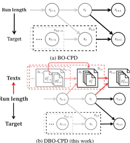
(a) BO-CPD
[image:2.595.77.289.59.292.2](b) DBO-CPD (this work)
Figure 1: This figures illustrates a graphical repre-sentation of BO-CPD and our DBO-CPD model.
xt, rt, andDt represent a continuous variable of
interest, the run length (hidden) variable, and doc-uments, respectively. Our modeling contribution is to add textsD1:t for the accurate prediction of
the run lengthrt+1.
Schumaker and Chen, 2009; Gid´ofalvi and Elkan, 2001; Fung et al., 2003; Fung et al., 2002; Schu-maker and Chen, 2006), tweets on Twitter (Si et al., 2013; Wang et al., 2012; Bollen et al., 2011; St Louis et al., 2012), online chats (Kim et al., 2010; Gruhl et al., 2005), and blog posts (Peng et al., 2015; Mishne and Glance, 2006).
In experiments, we show that DBO-CPD can ef-fectively distinguish whether an abrupt change is a change point or not in real-world datasets (see Sec-tion 3.1). Compared to previous BO-CPD models which explain the changes by human manual map-pings, our DBO-CPD automatically explains the reasons why a change point has occurred by con-necting the numerical sequence of data and textual features of news articles.
2 Bayesian Online Change Point Detection
This section will review our research problem, the change point detection (CPD) (Barry and Harti-gan, 1993), and the Bayesian Online Change Point Detection (BO-CPD) (Adams and MacKay, 2007) and our model, Document Based Online Change Point Detection (DBO-CPD).
Let xt∈R be a data observation at time t. We
assume that a sequence of data (x1, x2, ..., xt)
is composed of several non-overlapping produc-tive partitions (Barry and Hartigan, 1992). The boundaries that separate the partitions is called the change points. Letr be the random variable that denotes the run length, which is the number of time steps since the last change point was detected.
rt is the current run at timet. x(trt) denotes the
most recent data corresponding to the runrt.
2.1 Online Recursive Detection
To make an optimal prediction of the next data
xt+1, one may need to consider all possible run lengths rt∈N and a probability distribution over
run lengthrt. Given a sequence of data up to time t,x1:t = (x1, x2, ..., xt), the run length prediction
problem is formalized as computing the joint prob-ability of random variables P(xt+1, x1:t). This
distribution can be calculated in terms of the poste-rior distribution of run length at timet,P(rt|x1:t),
as follows:
P(xt+1, x1:t) = X
rt
P(xt+1|rt, xt(rt))P(rt|x1:t)
= X
rt
P(xt+1|x(trt))P(rt|x1:t).(1)
The predictive distribution P(xt+1|rt, x(trt))
de-pends only on the most recent rt observations x(rt)
t . The posterior distribution of run length P(rt|x1:t)can be computed recursively:
P(rt|x1:t) = PP(r(tx, x1:t)
1:t) (2)
where:
P(x1:t) = X
rt
P(rt, x1:t). (3)
The joint distribution over run lengthrtand data x1:t can be derived by summingP(rt, rt−1, x1:t)
overrt−1:
P(rt, x1:t) = X
rt−1
P(rt, rt−1, x1:t)
=X
rt−1
P(rt, xt|rt−1, x1:t−1)P(rt−1, x1:t−1)
=X
rt−1
P(rt|rt−1)P(xt|rt−1, x(trt))P(rt−1, x1:t−1).
However, the existing BO-CPD model (Adams and MacKay, 2007) specifies the conditional prior on the change pointP(rt|rt−1)in advance. This approach may lead to model biased predictions be-cause the update formula highly relies on the pre-defined, fixed hazard rate (h). Furthermore, BO-CPD is incapable of incorporating external infor-mation that implicitly influences the observation and explains the reasons for the current change of the long-term trend.
Figure 2: This figure illustrates the recursive up-dates of the posterior probability in the DBO-CPD model. Even the BO-CPD model only uses current and previous run length to calculate the posterior, DBO-CPD can utilize the series of text documents to compute the conditional probability accurately.
2.2 Document-based Bayesian Online Change Point Detection
This section explains our DBO-CPD model. To represent the text documents, we add a variableD which denotes a series of text documents related to the observed data as shown in Figure 1. Let
Dtbe a set ofNttext documentsDt1, D2t, ..., DtNt
that are indexed at time of publicationt, whereNt
is the number of documents observed at time t. Then, we can rewrite the joint probability over the run length as:
P(rt, x1:t) = X
rt−1
X
D(rt−1) t
Prt|rt−1, D(trt−1)
·
Pxt|rt−1, x(trt−1)
P(rt−1, x1:t−1) (4)
whereD(rt)
t (=Dt−rt+1:t)is the set of thertmost
recent documents. Figure 2 illustrates the recur-sive updates of posterior probability where solid lines indicate that the probability mass is passed upwards and dotted lines indicate the probability that the current run lengthrtis set to zero.
Given documentsD(rt)
t , the conditional
proba-bility is represented as follows:
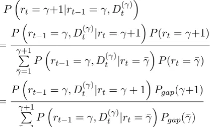
Prt=γ+1|rt−1 =γ, Dt(γ)
= P
rt−1 =γ, Dt(γ)|rt=γ+1
P(rt=γ+1) γP+1
¯
γ=1P
rt−1 =γ, D(tγ)|rt= ¯γ
P(rt= ¯γ)
= P
rt−1 =γ, Dt(γ)|rt=γ+ 1
Pgap(γ+1) γP+1
¯
γ=1P
rt−1 =γ, Dt(γ)|rt= ¯γ
Pgap(¯γ)
where Pgap is the distribution of intervals
be-tween consecutive change-points. As the BO-CPD model (Adams and MacKay, 2007), we assume the simplest case where the probability of a change-point at every step is constant if the length of a segment is modeled by a discrete exponential (ge-ometric) distribution as:
Pgap(rt|λ) =λexp−λrt (5)
whereλ > 0, arate parameter, is the parameter of the distribution.
The update rule for the prior distribution on rt
makes the computation of the joint distribution tractable,Pγγ¯+1=1P(rt−1=γ, Dt(γ)|rt=¯γ)·Pgap(¯γ).
Becausertcan only be increased toγ+ 1or set to
0, the conditional probability is as follows:
P(rt=γ+ 1|rt−1=γ, D(tγ))
= T TD(t, γ|γ+1)
D(t, γ|γ+1) +TD(t, γ|0)
(6)
where the function TD(t, α|α¯) is an
abbrevia-tion ofPrt−1=α, Dt(α)|rt=¯α
. In Equation (6),
TD(t, γ|γ+1)=P(rt−1=γ, D(tγ)|rt=γ+1) is the
joint probability of the run lengthrt−1 and a set of documentsD(tγ) when no change has occurred at timetand the run length becomesγ+ 1. There-fore, we can simplify the equation by removing
rt−1=γfrom the condition as follows:
TD(t, γ|γ+1) =P(Dt(γ)|rt=γ+ 1). (7)
We represent the distribution of words by the bag-of-words model. LetDi
t be the set of M words
that is part of the ith document at time t, i.e.
Di
t = {di,t1, di,t2, ..., di,Mt }. In the model, we
length parameterrt. In this setting, the conditional
probability of the words takes the following form:
PD(tγ)|rt=γ+1
= 1
Z Y
i,j
Pdi,jt |rt=γ+1
.
(8) The conditional probability P(di,jt |rt=γ+1) is
represented by two generative models, φwf and φwiwhich illustratesword frequencyandword im-pact, respectively. The key intuition ofword fre-quency is that a word tends to close to a change point if a word has been frequently seen in arti-cles, published when there was a rapid change. The key intuition of word impact is that how much does a word lose information in time which will be discussed in next section. In our paper, we use the unnormalized beta distribution of the weights of words to represent the exponential de-cays. The probabilityPD(tγ)|rt=γ+ 1
can be represented recursively as:
PD(γ)t |rt=γ+1
=PDt(γ)|γ+1
∝ φwi(Dt(γ)|γ+1)·φwf(Dt(γ)|γ+1) = φwi(Dt|γ+1)·φwf(Dt|γ+1)
·φwi(Dt(γ−−11)|rt−1=γ)·φwf(D(γt−−11)|rt−1=γ)
= Y
i,j
φwi(di,jt |γ+1)·φwf(di,jt |γ+1) (9)
·φwi(Dt(γ−−11)|rt−1=γ)·φwf(D(γt−−11)|rt−1=γ)
where:
φwf(dx,yt |γ) = count(d x,y
t , rt=γ) P
i,jcount(di,jt , rt=γ).
Here, φwi(dx,yt |γ) and φwf(dx,yt |γ) are empirical
potentials which contribute to representP(di,jt |γ).
φwi(·)is explained in Section 2.3. Here,count(E)
is the number of times event E appears in the dataset. In Equation (9), τt is the time gap
(dif-ference) betweentand the time when a document is generated, anddi,j represents a document
with-out considering the time domain.
TD(t, γ|0)is represented as follows:
P(rt−1=γ, Dt(γ)|rt=0)
=P(rt−1=γ|rt= 0)P(Dt(γ)|rt=0)
=H(γ+1)P(Dt(γ)|rt=0)
whereH(τ) is thehazard function (Forbes et al., 2011),
H(τ) = P∞Pgap(τ)
[image:4.595.307.535.78.297.2]t=τPgap(t). (10)
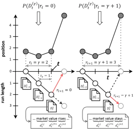
Figure 3: This figure illustrates how our Equa-tion (9) is calculated and how it determines whether a change occurs or not. If the same data is given, BO-CPD gives us the same answer to a question whether an abrupt change at time t is a change point or not. However, DBO-CPD uses documents Dtγ for its prediction to incorporate the external information which cannot be inferred only from the data.
WhenPgapis the discrete exponential distribution,
the hazard function is constant at H(τ) = 1/λ
(Adams and MacKay, 2007).
As an illustrative example, suppose that we found a rapid change in Google stock three days ago. Today at t = 3, we want to know how the articles are written and whether it will affect the change tomorrow (t = 4). As shown in Figure 3, we can calculate what degree a word, for example
rises orstays, is likely to appear in articles pub-lished since today, which isP(D(tγ)|rt = γ+1),
and this probability leads us to predict run lengths from the texts. Documents for eachτt= 0,1and
2.3 Generative Models Trained from Regression
LetD∈RT×N×M beN documents of news
arti-cles which consist ofM vocabulary over time do-mainT. Di
t∈RM is theith document of a set of
documents generated at timet, and definer∈RN
as the corresponding set of the run length, which is a time gap between the time when the document is generated and the next change point occurs. Then, given a text documentDi
t, we seek to predict the
value of run lengthrby learning a parameterized functionf:
ˆ
r=f(Di
t;w) (11)
wherew∈ Rdare the weights of text features for di,t1, di,t2, ..., di,Mt which compose documentsDi
t.
From a collection ofN documents, we use linear regression which is trained by solving the follow-ing optimization problem:
min
w,Di t
f(Dit;w)≡C
N X
i=1
ξ(w,Dit,rt) +r(w)
(12) where r(w) is the regularization term and
ξ(w,Di
t,rt)is the loss function. ParameterC >
0 is a user-specified constant for balancing r(w) and the sum of losses.
Let h be a function from a document into a vector-space representation∈Rd. In linear
regres-sion, the functionf takes the form:
f(Di
t;w) =h(Dti)>w+ (13)
whereis Gaussian noise.
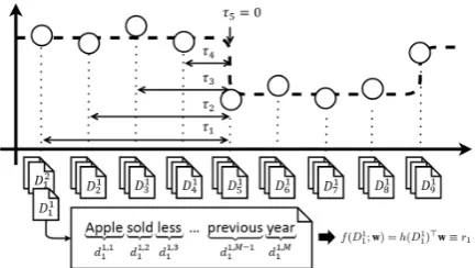
Figure 4 illustrates how we trained a linear re-gression model on a sample article. One issue is that the run length can not be trained directly. Suppose that we trainr5 = 0into regression, the weightwof the model will become 0 even though the set of words contained inDj5,∀j ∈ {1, ..., T} is composed of salient words which can incur a possible future change point. To solve this inter-pretability problem, we trained the weight in the inverse exponential domain for the predicted vari-able, predictinge−rt instead ofrt. In this setting,
the predicted run-length takes the form:
e−rˆt =h(D
t)>w+. (14)
[image:5.595.309.526.63.185.2]By this method, the regression model can give a high weight to a word which often appears close to change points. We can interpret that highly
Figure 4: This figure illustrates a graphical rep-resentation of how we train a generative model from a regression problem. We use a regression model to predict time gap rt between the release
date of article and the nearest future change point. The weights of regression model are changed into the negative exponential scale to be considered as
word impact.
weighted wordsd are more closely related to an outbreak of changes than lower weighted words.
With w, we can rewrite the probability ofd, τt
givenwas:
φwi(d, τt) ∝ wd·(exp(−1/wd))τt
= wd·exp(−τt/wd). (15)
The potential,φwi, can also be represented
recur-sively as follows:
φwi(d, τt+1) =φwi(d, τt)·exp(−1/wd), (16)
since given a wordd,τt+1=τt+1holds.
3 Experiments
Now we explain experiments of DBO-CPD in two real-world datasets, stock prices and movie rev-enues. The first case is the historical end-of-day stock prices of five information technology corpo-rations. In the second dataset, we examine daily film revenues averaged by the number of theaters.
3.1 Datasets
In the stock price dataset, we gather data for five different companies: Apple (AAPL), Google (GOOG), IBM (IBM), Microsoft (MSFT), and Facebook (FB). These companies were selected because they were the top 5 ranked in market value in 2015.
Figure 5: (a) Two plots show the results of BO-CPD (top) and DBO-CPD (middle) on Apple stock prices in January 2014. The stock price is plotted in light gray, with the predictive change points drawn as small circles. The red line represents the most likely predicted run-lengths for each day. Thebottom
figures are a set of visualizations of the top 15 strongly weighted words which are found at selected change points which BO-CPD is unable to predict. The size of each word represents the weight of its textual features learned during the training of the regression model.
and lead to many news articles. We use the his-torical stock price data from the Google Finance service.1.
category words documents words/doc
AAPL 15.0M 29,459 509
AAPL:N 11.0M 18,896 581
GOOG 15.0M 29,422 511
GOOG:N 8.2M 13,658 603
IBM 26.7M 45,741 583
IBM:N 3.4M 4,741 726
MSFT 20.5M 35,905 570
MSFT:N 3.5M 5,070 681
FB 18.9M 38,168 495
FB:N 4.3M 6,625 645
KNGHT 14.4M 16,874 852
INCPT 12.1M 17,155 705
AVGR 3.5M 6,476 537
FRZ 6.8M 15,021 454
[image:6.595.100.495.63.302.2]INTRS 4.2M 7,846 538
Table 1: Dimensions of the datasets used in this paper, after tokenizing and filtering the news ar-ticles. ‘:N’ means the articles are collected with additional ‘NASDAQ:’ search query.
The second dataset is a set of movie revenues averaged by the number of theaters for five months from the release date of film. We target 5 different
1https://www.google.com/finance
movies: The Dark Knight (KNGHT), Inception (INCPT), The Avengers (AVGR), Frozen (FRZ) and Interstellar (INTRS), because these movies are on highest-grossing movie list and also are screened recently. The cumulative daily revenue per theater is collected from ‘Box Office Mojo’ (www.boxofficemojo.com).
News articles are collected from Google News and we useGoogle search queriesto extract spe-cific articles related to each dataset in a spespe-cific time period. During the online article crawling, we store not only the titles of articles, HTML doc-uments, and publication dates, but also the num-ber of related articles. The numnum-ber of articles is used to differentiate the weight of news articles during the training of regression. In the case of stock price data, we use two different queries to decrease noise. First, we search with the company name such as ‘Google’. Then, we use queries spe-cific to stock ‘NASDAQ:’ to make the content of articles to be highly relevant to the stock market. In case of movie data, we search with the movie title with the additional word ‘movie’ to only col-lect articles related to the target movie.
[image:6.595.83.276.464.627.2]ar-ticle extractors, newspaper (Ou-Yang, 2013) and
python-goose (Grangier, 2013), to automate the text extraction of 291,057 HTML documents. Af-ter preprocessing, we could successfully extract texts from 287,389 (98.74%) HTMLs.
3.2 Textual Feature Representation
After extracting texts from HTMLs, we tokenize the texts into words. We use three different tok-enization methods which are downcasing the char-acters, punctuation removal, and removing En-glish stop words. Table 1 shows the statistics on the corpora of collected news articles.
With these article corpora, we use a bag-of-words(BoW) representation to change each word into a vector representation where words from ar-ticles are indexed and then weighted. Using these vectors, we adopt three document representations, TF, TFIDF, and LOG1P, which extend BoW rep-resentation. TF and TFIDF (Sparck Jones, 1972) calculate the importance of a word to a set of doc-uments based on term frequency. LOG1P (Kogan et al., 2009) calculates the logarithm of the word frequencies.
3.3 Training BO-CPD
As we noted earlier, we use BO-CPD to train the regression model to learn high weight for words which are more related to changes. When we choose the parameters for the Gaussian Process of BO-CPD, we try to find the value which makes the distance of intervals between predicted change points around 1-2 weeks. This is because we as-sume that the information included in the articles will have an immediate effect on the data right af-ter it is published to the public, so the exaf-ternal information in texts will indicate the short-term causes for a future change.
For the reasonable comparison of BO-CPD and DBO-CPD, we use the same parameter for the Gaussian Process in both models. After several experiments we found thata = 1andb = 1for the Gaussian Process andλgap= 250is
appropri-ate to train BO-CPD in the stock and film datasets. We separate the training and testing examples for cross-validation at a ratio of 2 : 1for each year. Then we train each model differently by year.
3.4 Learning the strength parameter w from Regression
The weightwof the regression model gives us an intuition of how a word is important which affect
2010 2011 2012 2013 2014
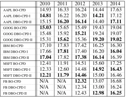
[image:7.595.307.525.61.230.2]AAPL BO-CPD 14.93 16.33 16.24 14.44 17.63 AAPL DBO-CPD I 14.81 16.22 16.20 14.21 17.12 AAPL DBO-CPD II 15.15 16.20 16.14 14.40 17.11 GOOG BO-CPD 15.03 15.65 15.49 19.43 19.04 GOOG DBO-CPD I 15.48 15.92 15.21 19.24 19.07 GOOG DBO-CPD II 15.31 15.62 15.36 19.20 19.02 IBM BO-CPD 17.10 17.83 17.42 16.25 16.30 IBM DBO-CPD I 17.66 17.81 17.40 16.20 16.04 IBM DBO-CPD II 17.04 17.82 17.38 16.14 16.39 MSFT BO-CPD 12.41 11.91 14.51 15.60 17.25 MSFT DBO-CPD I 12.33 12.60 14.48 14.92 16.43 MSFT DBO-CPD II 12.21 11.79 14.46 15.00 16.46 FB BO-CPD N/A N/A 12.32 13.07 16.68 FB DBO-CPD I N/A N/A 12.34 13.00 16.24 FB DBO-CPD II N/A N/A 12.43 12.98 16.25 Table 2: Negative log likelihood of five stocks (Apple, Google, IBM, Microsoft, and Facebook) without and with our model per year from 2010 to 2014. DBO-CPD I represents the experiments without ‘NASDAQ:’ as a search query and DBO-CPD II is the result of articles searched with ‘NASDAQ:’. Facebook data is not available be-fore the year 2012.
to the length of the current run. With the predicted run length calculated in Section 3.3, we change the run length domainr ∈ Rinto0 ≤r ≤1by pre-dictingertrather thanrtto solve the
interpretabil-ity problem. Therefore, we can think of a high weightwi as a powerful word which changes the
current run lengthr to0. To maintain the scala-bility ofw, we normalize the weight by rescaling the range intow ∈ [−1,1]. With the word rep-resentation calculated in Section 3.2, we train the regression model by using the number of relevant articles as the importance weight of training.
3.5 Results
We evaluate the performance of BO-CPD and DBO-CPD by comparing the negative log likeli-hood (NLL) (Turner et al., 2009) of two models at timetas:
logp(x1:T|w) = T X
t=1
logp(xt|x1:t−1,w).
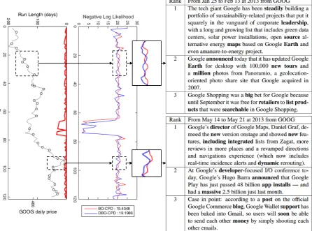
Figure 6: (b) Theleftplot illustrates daily stock prices of Google in 2013 from early January to late May. The black line represents the stock price, black circles indicate the predicted change points, and the red line shows the predicted run length calculated by DBO-CPD. Themiddleplot shows the negative log likelihood (NLL) of BO-CPD and DBO-CPD on the same data. The overall marginal NLL of DBO-CPD (19.1964) is smaller than BO-CPD (19.3438). The two zoomed intervals are the two longest intervals where the negative log likelihood of DBO-CPD is smaller than BO-CPD. The righttable shows the sentences whose run length predicted by the regression model (described in Section 2.3) are the highest at the two zoomed points, which means the sentences are likely to appear near feature change points. The boldface words are the top 5 most strongly-weighted terms in the regression model.
DBO-CPD compared to the BO-CPD is statisti-cally significant with 90% confidence in the four stocks except for stock of Facebook. We also found that most of the DBO-CPD II shows bet-ter results than DBO-CPD I and BO-CPD in most datasets due to noise reduction of texts through the additional search query ‘NASDAQ:’. Out of 23 datasets, APPL in 2010 and FB in 2012 are the only datasets where NLLs of BO-CPD is smaller (better) than NLLs of DBO-CPD.
One of the advantages of using a linear model is that we can investigate what the model discov-ers about different terms. As shown in Figure 5, we can find negative semantic words such as vi-cious,whip, anddesperately, and words
represent-ing the status of a company like propel, innova-tions, andgratefulare the most strongly-weighted terms in the regression model. We analyze and vi-sualize some change points where NLL of DBO-CPD is lower than NLL of BO-DBO-CPD. The results are shown in Figure 6 and three sentences are the top 3 most weighted sentences in the regression model for two changes with the boldface words of top 5 strongly weighted terms like the terms
[image:8.595.78.525.67.398.2]announce-NLL KNGHT BO-CPD 39.76 KNGHT DBO-CPD I 39.54 INCPT BO-CPD 55.60 INCPT DBO-CPD I 55.54 AVGR BO-CPD 32.12 AVGR DBO-CPD I 32.10
FRZ BO-CPD 51.25
FRZ DBO-CPD I 51.04
INT BO-CPD 38.49
[image:9.595.117.245.57.178.2]INT DBO-CPD I 38.31
Table 3: Negative log likelihood (NLL) of five movies (The Dark Knight, Inception, Avengers, Frozen, and Interstellar) without and with our model for 1 year from the release date of each movie.
ment the stock price increased. We can also find that the wordmillionis also a positive term which can predict a new change in the near feature. 4 Conclusions
In this paper, we propose a novel generative model for online inference to find change points from non-stationary time-series data. Unlike previ-ous approaches, our model can incorporate exter-nal information in texts which may includes the causes of signal changes. The main contribution of this paper is to combine the generative model for online change points detection and a regres-sion model learned from the weights of words in documents. Thus, our model accurately infers the conditional prior of the change points and auto-matically explains the reasons of a change by con-necting the numerical sequence of data and textual features of news articles.
5 Future work
Our DBO-CPD can be improved further by incor-porating more external information beyond docu-ments. In principle, our DBO-CPD can incorpo-rate other features if they are vectorized into a ma-trix form. Our implementation currently only uses the simple bag of words models (TF, TFIDF and LOG1P) to improve the baseline GP-based CPD models by bringing documents into change point detection. One possible direction of future work would explore ways to fully represent the rich in-formation in texts by extending the text features and language representations like continuous bag-of-words (CBOW) models (Mikolov et al., 2013) or Global vectors for word representation (GloVe) (Pennington et al., 2014).
Acknowledgments
This work was supported by Basic Science Research Program through the National Re-search Foundation of Korea (NRF) grant funded by the Ministry of Science, ICT & Future Planning (MSIP) (NRF- 2014R1A1A1002662), the NRF grant funded by the MSIP (NRF-2014M2A8A2074096).
References
Ryan Prescott Adams and David JC MacKay. 2007. Bayesian online changepoint detection. arXiv preprint arXiv:0710.3742.
Daniel Barry and John A Hartigan. 1992. Product par-tition models for change point problems. The An-nals of Statistics, pages 260–279.
Daniel Barry and John A Hartigan. 1993. A bayesian analysis for change point problems. Journal of the American Statistical Association, 88(421):309–319. Johan Bollen, Huina Mao, and Xiaojun Zeng. 2011. Twitter mood predicts the stock market. Journal of Computational Science, 2(1):1–8.
Jie Chen and AK Gupta. 1997. Testing and locat-ing variance changepoints with application to stock prices. Journal of the American Statistical Associa-tion, 92(438):739–747.
Siddhartha Chib. 1998. Estimation and comparison of multiple change-point models. Journal of econo-metrics, 86(2):221–241.
Pao-Shin Chu and Xin Zhao. 2004. Bayesian change-point analysis of tropical cyclone activity: The central north pacific case. Journal of Climate, 17(24):4893–4901.
Catherine Forbes, Merran Evans, Nicholas Hastings, and Brian Peacock. 2011. Statistical distributions. John Wiley & Sons.
Gabriel Pui Cheong Fung, Jeffrey Xu Yu, and Wai Lam. 2002. News sensitive stock trend prediction. InAdvances in knowledge discovery and data min-ing, pages 481–493. Springer.
Gabriel Pui Cheong Fung, Jeffrey Xu Yu, and Wai Lam. 2003. Stock prediction: Integrating text min-ing approach usmin-ing real-time news. InIEEE Inter-national Conference on Computational Intelligence for Financial Engineering, pages 395–402.
Gyozo Gid´ofalvi and Charles Elkan. 2001. Us-ing news articles to predict stock price movements.
Department of Computer Science and Engineering, University of California, San Diego.
Daniel Gruhl, Ramanathan Guha, Ravi Kumar, Jasmine Novak, and Andrew Tomkins. 2005. The predic-tive power of online chatter. InProceedings of the Eleventh ACM SIGKDD International Conference on Knowledge Discovery and Data Mining, pages 78–87.
William Gu, Jaesik Choi, Ming Gu, Horst Simon, and Kesheng Wu. 2013. Fast change point detection for electricity market analysis. In IEEE International Conference on Big Data, pages 50–57.
Der-Ann Hsu. 1977. Tests for variance shift at an un-known time point. Applied Statistics, pages 279– 284.
Su Nam Kim, Lawrence Cavedon, and Timothy Bald-win. 2010. Classifying dialogue acts in one-on-one live chats. In Proceedings of the 2010 Con-ference on Empirical Methods in Natural Language Processing, pages 862–871.
Shimon Kogan, Dimitry Levin, Bryan R Routledge, Ja-cob S Sagi, and Noah A Smith. 2009. Predicting risk from financial reports with regression. In Pro-ceedings of Human Language Technologies: Con-ference of the North American Chapter of the Asso-ciation for Computational Linguistics, pages 272– 280.
Gary Koop and Simon M. Potter. 2007. Estimation and forecasting in models with multiple breaks. The Review of Economic Studies, 74(3):pp. 763–789. Tomas Mikolov, Kai Chen, Greg Corrado, and
Jef-frey Dean. 2013. Efficient estimation of word representations in vector space. arXiv preprint arXiv:1301.3781.
Gilad Mishne and Natalie S Glance. 2006. Predicting movie sales from blogger sentiment. InAAAI Spring Symposium: Computational Approaches to Analyz-ing Weblogs, pages 155–158.
Joel Nothman, Matthew Honnibal, Ben Hachey, and James R Curran. 2012. Event linking: Grounding event reference in a news archive. InProceedings of the 50th Annual Meeting of the Association for Computational Linguistics (ACL), pages 228–232. Michael Osborne. 2010.Bayesian Gaussian processes
for sequential prediction, optimisation and quadra-ture. Ph.D. thesis, Oxford University New College. Lucas Ou-Yang. 2013. newspaper - news, full-text,
and article metadata extraction.
Baolin Peng, Jing Li, Junwen Chen, Xu Han, Ruifeng Xu, and Kam-Fai Wong. 2015. Trending sentiment-topic detection on twitter. In Computational Lin-guistics and Intelligent Text Processing, pages 66– 77. Springer.
Jeffrey Pennington, Richard Socher, and Christopher D Manning. 2014. Glove: Global vectors for word representation. Proceedings of the Empiricial
Methods in Natural Language Processing (EMNLP 2014), 12:1532–1543.
Robert Schumaker and Hsinchun Chen. 2006. Textual analysis of stock market prediction using financial news articles. AMCIS 2006 Proceedings, page 185. Robert P Schumaker and Hsinchun Chen. 2009.
Textual analysis of stock market prediction using breaking financial news: The azfin text system.
ACM Transactions on Information Systems (TOIS), 27(2):12.
Jianfeng Si, Arjun Mukherjee, Bing Liu, Qing Li, Huayi Li, and Xiaotie Deng. 2013. Exploiting topic based twitter sentiment for stock prediction. AFM Smith. 1975. A bayesian approach to inference
about a change-point in a sequence of random vari-ables. Biometrika, 62(2):407–416.
Karen Sparck Jones. 1972. A statistical interpretation of term specificity and its application in retrieval.
Journal of documentation, 28(1):11–21.
Connie St Louis, Gozde Zorlu, et al. 2012. Can twitter predict disease outbreaks? BMJ, 344.
DA Stephens. 1994. Bayesian retrospective multiple-changepoint identification. Applied Statistics, pages 159–178.
Mark Steyvers and Scott Brown. 2005. Prediction and change detection. InAdvances in Neural Informa-tion Processing Systems (NIPS), pages 1281–1288. Ryan Turner, Yunus Saatci, and Carl Edward
Ras-mussen. 2009. Adaptive sequential bayesian change point detection.
Udo von Toussaint. 2011. Bayesian inference in physics. Reviews of Modern Physics, 83(3):943. Hao Wang, Dogan Can, Abe Kazemzadeh, Franc¸ois
Bar, and Shrikanth Narayanan. 2012. A system for real-time twitter sentiment analysis of 2012 us pres-idential election cycle. InProceedings of the ACL 2012 System Demonstrations, pages 115–120. As-sociation for Computational Linguistics.
Xiang Xuan and Kevin Murphy. 2007. Modeling changing dependency structure in multivariate time series. In Proceedings of the 24th International Conference on Machine Learning (ICML), pages 1055–1062.
Xin Zhao and Pao-Shin Chu. 2010. Bayesian change-point analysis for extreme events (typhoons, heavy rainfall, and heat waves): An rjmcmc approach.