Fast Large Scale Approximate Graph Construction for NLP

Fast Large-Scale Approximate Graph Construction for NLP

Amit Goyal and Hal Daum´e III Dept. of Computer Science

University of Maryland

College Park, MD

{amit,hal}@umiacs.umd.edu

Raul Guerra

Dept. of Computer Science University of Maryland

College Park, MD

[email protected]

Abstract

Many natural language processing problems involve constructing large nearest-neighbor graphs. We propose a system called FLAG to construct such graphs approximately from large data sets. To handle the large amount of data, our algorithm maintains approximate counts based on sketching algorithms. To find the approximate nearest neighbors, our algorithm pairs a new distributed online-PMI algorithm with novel fast approximate near-est neighbor search algorithms (variants of PLEB). These algorithms return the approxi-mate nearest neighbors quickly. We show our system’s efficiency in both intrinsic and ex-trinsic experiments. We further evaluate our fast search algorithms both quantitatively and qualitatively on two NLP applications.

1 Introduction

Many natural language processing (NLP) prob-lems involve graph construction. Examples in-clude constructing polarity lexicons based on lexi-cal graphs from WordNet (Rao and Ravichandran, 2009), constructing polarity lexicons from web data (Velikovich et al., 2010) and unsupervised part-of-speech tagging using label propagation (Das and Petrov, 2011). The later two approaches con-struct nearest-neighbor graphs between word pairs by computing nearest neighbors between word pairs from large corpora. These nearest neighbors form the edges of the graph, with weights given by the distributional similarity (Turney and Pantel, 2010) between terms. Unfortunately, computing the distri-butional similarity between all words in a large vo-cabulary is computationally and memory intensive

when working with large amounts of data (Pantel et al., 2009). This bottleneck is typically addressed by means of commodity clusters. For example, Pantel et al. (2009) compute distributional similarity be-tween500million terms over a200billion words in 50hours using100quad-core nodes, explicitly stor-ing a similarity matrix between500million terms.

In this work, we propose Fast Large-Scale Ap-proximate Graph (FLAG) construction, a sys-tem that constructs a fast large-scale approximate nearest-neighbor graph from a large text corpus. To build this system, we exploit recent developments in the area of approximation, randomization and streaming for large-scale NLP problems (Ravichan-dran et al., 2005; Goyal et al., 2009; Levenberg et al., 2010). More specifically we exploit work on Lo-cality Sensitive Hashing (LSH) (Charikar, 2002) for computing word-pair similarities from large text col-lections (Ravichandran et al., 2005; Van Durme and Lall, 2010). However, Ravichandran et al. (2005) approach stored an enormous matrix of all unique words and their contexts in main memory, which is infeasible for very large data sets. A more efficient online framework to locality sensitive hashing (Van Durme and Lall, 2010; Van Durme and Lall, 2011) computes distributional similarity in a streaming set-ting. Unfortunately, their approach can handle only additive features like raw-counts, and not non-linear association scores like pointwise mutual information (PMI), which generates better context vectors for distributional similarity (Ravichandran et al., 2005; Pantel et al., 2009; Turney and Pantel, 2010).

In FLAG, we first propose a novel distributed online-PMI algorithm (Section 3.1). It is a stream-ing method that processes large data sets in one pass while distributing the data over commodity clusters

and returns context vectors weighted by pointwise mutual information (PMI) for all the words. Our distributed online-PMI algorithm makes use of the Count-Min (CM) sketch algorithm (Cormode and Muthukrishnan, 2004) (previously shown effective for computing distributional similarity in our ear-lier work (Goyal and Daum´e III, 2011)) to store the counts of all words, contexts and word-context pairs using only8GBof main memory. The main motiva-tion for using the CM sketch comes from its linear-ity property (see last paragraph of Section 2) which makes CM sketch to be implemented in distributed setting for large data sets. In our implementation,

FLAGscaled up to 110GB of web data with 866 million sentences in less than2days using100 quad-core nodes. Our intrinsic and extrinsic experiments demonstrate the effectiveness of distributed online-PMI.

After generating context vectors from distributed online-PMI algorithm, our goal is to use them to find fast approximate nearest neighbors for all words. To achieve this goal, we exploit recent developments in the area of existing randomized algorithms for ran-dom projections (Achlioptas, 2003; Li et al., 2006), Locality Sensitive Hashing (LSH) (Charikar, 2002) and improve on previous work done on PLEB(Point

Location in Equal Balls) (Indyk and Motwani, 1998; Charikar, 2002). We propose novel variants of PLEB

to address the issue of reducing the pre-processing time for PLEB. One of the variants of PLEB(FAST -PLEB) with considerably less pre-processing time has effectiveness comparable to PLEB. We evaluate these variants of PLEBboth quantitatively and qual-itatively on large data sets. Finally, we show the ap-plicability of large-scale graphs built fromFLAGon two applications: the Google-Sets problem (Ghahra-mani and Heller, 2005), and learning concrete and abstract words (Turney et al., 2011).

2 Count-Min sketch

The Count-Min (CM) sketch (Cormode and Muthukrishnan, 2004) belongs to a class of ‘sketch’ algorithms that represents a large data set with a compact summary, typically much smaller than the full size of the input by processing the data in one pass. The following surveys comprehensively review the streaming literature (Rusu and Dobra,

2007; Cormode and Hadjieleftheriou, 2008) and sketch techniques (Charikar et al., 2004; Li et al., 2008; Cormode and Muthukrishnan, 2004; Rusu and Dobra, 2007). In our another recent paper (Goyal et al., 2012), we conducted a systematic study and compare many sketch techniques which answer point queries with focus on large-scale NLP tasks. In that paper, we empirically demonstrated that CM sketch performs the best among all the sketches on three large-scale NLP tasks.

CM sketch uses hashing to store the approximate frequencies of all items from the large data set onto a small sketch vector that can be updated and queried in constant time. CM has two parametersandδ:

controls the amount of tolerable error in the returned count andδ controls the probability with which the error exceeds the bound.

CM sketch with parameters (,δ) is represented as a two-dimensional array with widthwand depth

d; where wandddepends on andδ respectively. We set w=2 and d=log(1_δ). The depth d denotes the number of pairwise-independent hash functions employed by the CM sketch; and the widthw de-notes the range of the hash functions. Given an input stream of items of length N (x1,x2. . .xN), each of the hash functions hk:{x1,x2. . .xN} →

{1. . . w},∀1 ≤ k ≤ d, takes an item from the in-put stream and maps it into a position indexed by the corresponding hash function.

UPDATE: For each new item “x” with countc, the sketch is updated as:

sketch[k, hk(x)]←sketch[k, hk(x)]+c, ∀1≤k≤d.

QUERY: Since multiple items can be hashed to the

same index for each row of the array, hence the stored frequency in each row is guaranteed to over-estimatethe true count, which makes it a biased esti-mator. Therefore, to answer the point query (QUERY

(x)), CM returns the minimum over all thed posi-tions indexed by the hash funcposi-tions.

ˆ

c(x) = mink sketch[k, hk(x)], ∀1≤k≤d.

All reported frequencies by CM exceed the true frequencies by at most N with probability of at least 1 −δ. The space used by the algorithm is

O(1log1_δ). Constant time of O(log(1_δ)) per each

update and query operation.

(us-ing the same parameterswandd, and the same set ofdhash functions) over different input streams; the sketch of the combined data stream can be easily ob-tained by adding the individual sketches in O(d×w) time which is independent of the stream size. This property enables sketches to be implemented in dis-tributed setting, where each machine computes the sketch over a small portion of the corpus and makes itscalableto large datasets.

The idea of conservative update (Estan and Vargh-ese, 2002) is to only increase counts in the sketch by the minimum amount needed to ensure that the estimate remains accurate. We (Goyal and Daum´e III, 2011) used CM sketch with conservative update (CM-CU sketch) to show that the update reduces the amount of over-estimation error by a factor of at least 1.5 on NLP data and showed the effective-ness of CM-CU on three important NLP tasks. The

QUERYprocedure for CM-CU is identical to

Count-Min. However, to UPDATE an item “x” with fre-quencyc, first we compute the frequencycˆ(x)of this item from the existing data structure:

(∀1≤k≤d,cˆ(x) = mink sketch[k, hk(x)])

and the counts are updated according to:

sketch[k, hk(x)]←max{sketch[k, hk(x)],ˆc(x) +c}. The intuition is that, since the point query returns the minimum of all the d values, we will update a counter only if it is necessary as indicated by the above equation. This heuristic avoids the unnecessary updating of counter values to reduce the over-estimation error.

3 FLAG: Fast Large-Scale Approximate Graph Construction

We describe a system,FLAG, for generating a near-est neighbor graph from a large corpus. For ev-ery node (word), our system returns top l approxi-mate nearest neighbors, which implicitly defines the graph. Our system operates in four steps. First, for every word “z”, our system generates a sparse con-text vector (h(c1, v1); (c2, v2). . .; (cd, vd)i) of size

dwhere cd denotes the context and vd denotes the PMI (strength of association) between the context cd and the word “z”. The context can be lexical, semantic, syntactic, and/or dependency units that co-occur with the word “z”. We compute this

ef-ficiently using a new distributed online Pointwise Mutual Information algorithm (Section 3.1). Sec-ond, we project all the words with context vector sizedontokrandom vectors and then binarize these random projection vectors (Section 3.2). Third, we propose novel variants of PLEB (Section 3.3) with less pre-processing time to represent data for fast query retrieval. Fourth, using the output of vari-ants of PLEB, we generate a small set of potential nearest neighbors for every word “z” (Section 3.4). From this small set, we can compute the Hamming distance between every word “z” and its potential nearest neighbors to return thel nearest-neighbors for all unique words.

3.1 Distributed online-PMI

We propose anewdistributed online Pointwise Mu-tual Information (PMI) algorithm motivated by the online-PMI algorithm (Van Durme and Lall, 2009b) (page 5). This is a streaming algorithm which pro-cesses the input corpus in one pass. After one pass over the data set, it returns the context vec-tors for all query words. The original online-PMI algorithm was used to find the top-d verbs for a query verb using the highest approximate online-PMI values using a Talbot-Osborne-Morris-Bloom1 (TOMB) Counter (Van Durme and Lall, 2009a). Unfortunately, this algorithm is prohibitively slow when computing contexts forallwords, rather than just a small query set. This motivates us to propose a distributed variant that enables us to scale to large data and large vocabularies.2

We make three modifications to the original online-PMI algorithm and refer to it as the “modified online-PMI algorithm” shown in Algorithm 1. First, we use Count-Min with conservative update (CM-CU) sketch (Goyal and Daum´e III, 2011) instead of TOMB. We prefer CM because it enables distribu-tion due to its linearity property (Secdistribu-tion 2) and foot-note #1. Distribution using TOMB is not known in literature and we will like to explore that direction in future. Second, we store the counts of words (“z”), contexts (“y”) and word-context pairs all together in

1

TOMB is a variant of CM sketch which focuses on reduc-ing the bit size of each counter (in addition to the number of counters) at the cost of incurring more error in the counts.

Algorithm 1Modified online-PMI

Require: Data setD, buffer sizeB

Ensure: context vectorsV, mapping word z to d-best contexts in priority queuehy,PMI(z,y)i

1: initialize CM-CU sketch to store approximate counts of words, context and word-context pairs

2: foreach bufferBin the data setDdo 3: initializeSto storehz,yiobserved inB

4: for hz,yiinBdo 5: set S (hz,yi) =1

6: insert z, y and pairhz,yiin sketch

7: end for

8: forx in setSdo

9: recompute vectors V(x) using current contexts in priority queue and{y|S(hz,yi)=1}

10: end for 11: end for

12: return context vectorsV

the CM-CU sketch (in the original online-PMI al-gorithm, exact counts of words and contexts were stored in a hash table; only the pairs were stored in the TOMB data structure). Third, in the original al-gorithm, for each “z” a vector of top-dcontexts are modified at the end of each buffer (refer Algorithm 1). However, in our algorithm, we only modify the list of those “z”’s which appeared in the recent buffer rather than modifying for all the “z”’s (Note, if “z” does not appear in the recent buffer, then its top-d

contexts cannot be changed. Hence, we only modify those “z”s which appear in the recent buffer).

In our distributed online-PMI algorithm, first we split the data into chunks of 10 million sentences. Second, we run the modified online-PMI algorithm on each chunk in distributed setting. This stores counts of all words (“z”), contexts (“y”) and word-context pairs in the CM-CU sketch, and store top-d

contexts for each word in priority queues. In third step, we merge all the sketches using linearity prop-erty to sum the counts of the words, contexts and word-context pairs. Additionally we merge the lists of top-dcontexts for each word. In the last step, we use the single merged sketch and merged top-d con-texts list to generate the final distributed online-PMI top-dcontexts list.

It takes around one day to compute context vec-tors for all the words from a chunk of 10 million sentences using first step of distributed online-PMI. We generated context vectors for all the87 chunks

(110GB data with 866 million sentences: see Table 1) in one day by running one process per chunk over a cluster. The first step of the algorithm involves traversing the data set and is the most time intensive step. For the second step, the merging of sketches is fast, since sketches are two dimensional array data structures (we used the sketch of size2billion coun-ters with3hash functions). Merging the lists of

top-dcontexts for each word is embarrassingly parallel and fast. The last step to generate the final top-d

contexts list is again embarrassingly parallel and fast and takes couple of hours to generate the top-d con-texts for all the words from all the chunks. If im-plemented serially the “modified online-PMI algo-rithm” on 110GB data with 866 million sentences would take approximately3months.

The downside of the distributed online-PMI is that it splits the data into small chunks and loses infor-mation about the global best contexts for a word over all the chunks. The algorithm locally computes the best contexts for each chunk, that can be bad if the algorithm misses out globallygoodcontexts and that can affect the accuracy of downstream applica-tion. We will demonstrate in our experiments (Sec-tion 4.2) by using distributed online-PMI, we do not lose any significant information about global con-texts and perform comparable to offline-PMI over an intrinsic and extrinsic evaluation.

3.2 Dimensionality Reduction fromRD toRk

We are given context vectors forZ words, our goal is to use k random projections to project the con-text vectors from RD to Rk. There are total D

unique contexts (D >> k) for all Z words. Let (h(c1, v1); (c2, v2). . .; (cd, vd)i) be sparse context vectors of sizedforZwords. For each word, we use hashing to project the context vectors ontok direc-tions. We usekpairwise independent hash functions that maps each of thedcontext (cd) dimensions onto

βd,k ∈ {−1,+1}; and compute inner product be-tweenβd,kandvd. Next,∀k,

P

dβd,k.vdreturns the

krandom projections for each word “z”. We store thek random projections for all words (mapped to integers) as a matrixAof size ofk×Z.

    

1 2 · · · Z k1 hz1, 26i hz2,80i · · · hzZ, 3i

k2 hz1,−28i hz2, 6i · · · hzZ,111i

..

. ... ... . .. ... kK hz1, 78i hz2,69i · · · hzZ,92i

     Sort₌ ⇒

(a) MatrixA

    

Smallest to Largest

hzZ, 3i hz1,26i · · · hzm,700i hzr,−50i hz2, 6i · · · hzZ,111i

..

. ... . .. ...

hz1,78i hzZ,92i · · · hzu,432i

     ⇒

(b) MatrixA

    

1 2 · · · Z zZ z1 · · · zm zr z2 · · · zZ

..

. ... . .. ... z1 zZ · · · zu

     ⇒

(c) MatrixA

   

z1 z2 · · · zZ 2 60 · · · 1 55 2 · · · Z

..

. ... . .. ... 1 90 · · · 2

   

(d) MatrixC

Figure 1: First matrix pairs the words1· · ·Zand their random projection values. Second matrix sorts each row by the random projection values from smallest to largest. Third matrix throws away the projection values leaving only the words. Fourth matrix maps the words1· · ·Zto their sorted position in the third matrix for eachk. This allows constant query time for all the words.

is motivated by the work on stable random projec-tions (Li et al., 2006; Li et al., 2008), Count sketch (Charikar et al., 2004), feature hashing (Weinberger et al., 2009) and online Locality Sensitive Hashing (LSH) (Van Durme and Lall, 2010). The idea of gen-erating random projections from the set {−1,+1}

was originally proposed by Achlioptas (2003). Next we create a binary matrix B using matrix

A by taking sign of each of the entries of the

ma-trix A. If A(i, j) ≥ 0, then B(i, j) = 1; else

B(i, j) = 0. This binarization creates Locality

Sen-sitive Hash (LSH) function that preserves the cosine similarity between every pair of word vectors. This idea was first proposed by Charikar (2002) and used in NLP for large-scale noun clustering (Ravichan-dran et al., 2005). However, in large-scale noun clustering work, their approach had to store the ran-dom projection matrix of sizeD×k; whereD de-notes the number of all unique contexts (which is generally large andD >> Z) and in this paper, we do not explicitly require storing a random projection matrix.

3.3 Representation for Fast-Search

We describe three approaches to represent the data (matrixAandBfrom Section 3.2) in such a manner that finding nearest neighbors is fast. These three approaches differ in amount of pre-processing time. First, we propose a naive baseline approach using random projections independently with the best pre-processing time. Second, we describe PLEB (Point

Location in Equal Balls) (Indyk and Motwani, 1998; Charikar, 2002) with the worst pre-processing time. Third, we propose a variant of PLEB to reduce its

pre-processing time.

3.3.1 Independent Random Projections (IRP)

Here, we describe a naive baseline approach to arrange nearest neighbors next to each other by

us-ing Independent Random Projections (IRP). In this

approach, we pre-process the matrix A. First for matrixA, we pair the wordsz1· · ·zZand their ran-dom projection values as shown in Fig. 1(a). Sec-ond, we sort the elements of each row of matrixA

by their random projection values from smallest to largest (shown in Fig. 1(b)). The sorting step takes

O(ZlogZ)time (We can assumekto be a constant). The sorting operation puts all the nearest neighbor words (for eachk independent projections) next to each other. After sorting the matrix A, we throw away the projection values leaving only the words (see Fig. 1(c)). To search for a word in matrix A

in constant time, we create another matrixCof size (k×Z) (see Fig. 1(d)). MatrixC maps the words

z1· · ·zZto their sorted position in the matrixA(see Fig. 1(c)) for eachk.

3.3.2 PLEB

PLEB (Point Location in Equal Balls) was first proposed by Indyk and Motwani (1998) and further improved by Charikar (2002). The improved PLEB

algorithm puts in operationallkrandom projections together. It randomly permutes the ordering ofk bi-nary LSHbits (stored in matrixB) for all the words

ptimes. For each permutation it sorts all the words lexicographically based on their permuted LSH

rep-resentation of sizek. The sorting operation puts all the nearest neighbor words (usingkprojections to-gether) next to each other for all the permutations. In practicepis generally large, Ravichandran et al. (2005) usedp= 1000in their work.

In our implementation of PLEB, we have a matrix

a matrixCof size (p×Z) is used to map the words 1· · ·Zto their sorted position in the matrixA. Note, in IRPapproach, the size ofAandCmatrix is (k× Z). In PLEB generating random permutations and sorting the bit vectors of sizekinvolves worse pre-processing time than using IRP. However, spending more time in pre-processing leads to finding better approximate nearest neighbors.

3.3.3 FAST-PLEB

To reduce the pre-processing time for PLEB, we propose a variant of PLEB (FAST-PLEB). In PLEB, while generating random permutations, it uses all thek bits. In this variant, for each random permu-tation we randomly sample without replacement q

(q << k) bits out of k. We use q bits to repre-sent each permutation and sort based on theseqbits. This makes pre-processingfasterfor PLEB. Section 4.3 shows that FAST-PLEB only needs q = 10to perform comparable to PLEB withq = 3000(that makes FAST-PLEB 300 times faster than PLEB). Here, again we store matrices A and C of size (p×Z).

3.4 Finding Approximate Nearest Neighbors

The goal here is to exploit three representations dis-cussed in Section 3.3 to find approximate nearest neighbors quickly. For all the three methods (IRP, PLEB, FAST-PLEB), we can use the same fast ap-proximate search which is simple and fast. To search a word “z”, first, we can look up matrixCto locate thekpositions where “z” is stored in matrixA. This can be done in constant time (Again assumingk(for IRP) andp(for PLEB and FAST-PLEB) to be a con-stant.). Once, we find “z” in each row, we can select

b(beam parameter) neighbors (b/2 neighbors from left andb/2neighbors from right of the query word.) for all thekorprows. This can be done in constant time (Assumingk, p and bto be constants.). This search procedure produces a set of bk (IRP) or bp

(PLEBand FAST-PLEB) potential nearest neighbors for a query word “z”. Next, we compute Hamming distance between query word “z” and the set of po-tential nearest neighbors from matrix B to return l

closest nearest neighbors. For computing hamming distance, all the approaches discussed in Section 3.3 require allkrandom projection bits.

4 Experiments

We evaluate our systemFLAGfor fast large-scale approximate graph construction. First, we show that using distributed online-PMI algorithm is as effec-tive as offline-PMI. Second, we compare the approx-imate nearest neighbors lists generated by FLAG

against the exact nearest neighbor lists. Finally, we show the quality of our approximate similarity lists generated byFLAGfrom the web corpus.

4.1 Experimental Setup

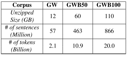
Data sets: We use two data sets: Gigaword (Graff, 2003) and a copy of news web (Ravichandran et al., 2005). For both the corpora, we split the text into sentences, tokenize and convert into lower-case. To evaluate our approximate graph construction, we evaluate on three data sets: Gigaword (GW), Giga-word +50% of web data (GWB50) and Gigaword +100%((GWB100)) of web data. Corpus statistics are shown in Table 1. We define the context for a given word “z” as the surrounding words appearing in a window of 2 words to the left and 2 words to the right. The context words are concatenated along with their positions -2, -1, +1, and +2.

Corpus GW GWB50 GWB100

Unzipped

12 60 110

Size (GB)

#of sentences

57 463 866

(Million)

#of tokens

2.1 10.9 20.0

(Billion)

Table 1:Corpus Description

4.2 Evaluating Distributed online-PMI

with 3 hash functions. In second pass, using the aggregated counts from the sketch, we generate the offline-PMI vectors of sized= 1000for every word. For rest of this paper for distributed online-PMI, we

setd= 1000and the size of the buffer=10,000and

we split the data sets into small chunks of10million sentences.

Intrinsic Evaluation: We use four kinds of mea-sures: precision (P), recall (R), f-measure (F1) and Pearson’s correlation (ρ) to measure the overlap in the context vectors obtained using online and offline PMI.ρis computed between contexts that are found in offline and online context vectors. We do this evaluation on447words selected from the concate-nation of four test-sets mentioned in the next para-graph. On these447words, we achieve an average P

of.97, average R of.96and average F1 of.97and a

perfect averageρof1. This evaluation show that the vectors obtained using online-PMI are as effective as offline-PMI.

Extrinsic Evaluation: We also compare online-PMI effectiveness on four test sets which consist of word pairs, and their corresponding human rank-ings. We generate the word pair rankings using online-PMI and offline-PMI strategies. We report the Pearson’s correlation (ρ) between the human and system generated similarity rankings. The four test sets are: WS-353 (Finkelstein et al., 2002) is a set of353word pairs. WS-203: A subset of WS-353 with 203 word pairs (Agirre et al., 2009). RG-65: (Rubenstein and Goodenough, 1965) has 65 word pairs. MC-30: A subset of RG-65 dataset with30 word pairs (Miller and Charles, 1991).

The results in Table 2 shows that by using dis-tributed online-PMI (by making a single pass over the corpus) is comparable to offline-PMI (which is computed by making two passes over the corpus).

For generating context vectors fromGW, for both offline-PMI and online-PMI, we use a frequency cutoff of5for word-context pairs to throw away the rare terms as they are sensitive to PMI (Church and Hanks, 1989). Next, FLAGgenerates online-PMI

vectors from GWB50 andGWB100 and uses

fre-quency cutoffs of15 and25. The higher frequency cutoffs are selected based on the intuition that, with more data, we get more noise, and hence not con-sidering word-context pairs with frequency less than 25 will be better for the system. AsFLAG is

go-ing to use the context vectors to find nearest neigh-bors, we also throw away all those words which have

≤50contexts associated with them. This generates context vectors for57,930words fromGW;95,626 fromGWB50and106,733fromGWB100.

Test Set WS-353 WS-203 RG-65 MC-30

Offline-PMI .41 .55 .40 .52

Online-PMI .41 .56 .39 .51

Table 2:Evaluating word pairs ranking with online and offline PMI. Scores are evaluated usingρmetric.

10 25 50 100

R ρ R ρ R ρ R ρ

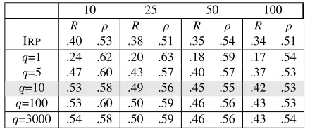
IRP .40 .53 .38 .51 .35 .54 .34 .51 q=1 .24 .62 .20 .63 .18 .59 .17 .54 q=5 .47 .60 .43 .57 .40 .57 .37 .53 q=10 .53 .58 .49 .56 .45 .55 .42 .53 q=100 .53 .60 .50 .59 .46 .56 .43 .53 q=3000 .54 .58 .50 .59 .46 .56 .43 .54

Table 4: Varying parameterqfor FAST-PLEBwith fixedp= 1000,k= 3000andb= 40. Results reported on recall andρ.

4.3 Evaluating Approximate Nearest Neighbor

Experimental Setup: To evaluate approximate nearest neighbor similarity lists generated by

FLAG, we conduct three experiments. We evaluate all the three experiments on447words (test set) as used in Section 4.2. For each word, both exact and approximate methods returnl= 100nearest neigh-bors. The exact similarity lists for447test words is computed by calculating cosine similarity between 447test words with respect to all other words. We also compare the LSH (computed using Hamming distance between all words and test set.) approxi-mate nearest neighbor similarity lists against the ex-act similarity lists. LSH provides an upper bound on the performance of our approximate search rep-resentations (IRP, PLEB, and FAST-PLEB) for fast-search from Section 3.3) . We set the number of projectionsk = 3000for all three methods and for PLEB and FAST-PLEB, we set number of permuta-tionsp = 1000as used in large-scale noun cluster-ing work (Ravichandran et al., 2005).

IRP PLEB FAST-PLEB

10 25 50 100 10 25 50 100 10 25 50 100

R ρ R ρ R ρ R ρ R ρ R ρ R ρ R ρ R ρ R ρ R ρ R ρ

LSH .55 .57 .52 .56 .49 .54 .46 .52 .55 .57 .52 .56 .49 .54 .46 .52 .55 .57 .52 .56 .49 .54 .46 .52 20 .29 .50 .26 .55 .25 .54 .24 .50 .50 .59 .45 .60 .41 .57 .37 .55 .48 .58 .42 .58 .38 .58 .35 .55 30 .36 .55 .33 .56 .31 .55 .30 .52 .53 .59 .48 .59 .44 .56 .41 .54 .51 .57 .47 .57 .42 .56 .40 .54 40 .40 .53 .38 .51 .35 .54 .34 .51 .54 .58 .50 .59 .46 .56 .43 .54 .53 .58 .49 .56 .45 .55 .42 .53 50 .44 .56 .42 .54 .39 .54 .37 .52 .54 .58 .51 .57 .47 .56 .44 .53 .54 .58 .50 .56 .46 .55 .44 .53 100 .53 .59 .49 .54 .46 .55 .43 .53 .55 .56 .52 .56 .48 .54 .46 .53 .55 .57 .52 .56 .48 .54 .46 .53

Table 3: Evaluation results on comparing LSH, IRP, PLEB, and FAST-PLEBwithk = 3000andb={20,30,40,50,100}with exact nearest neighbors overGWdata set. For PLEBand FAST-PLEB, we setp= 1000and for FAST-PLEB, we setq= 10. We report results on recall (R) andρmetric. For IRP, we sample firstprows and only useprows rather thank.

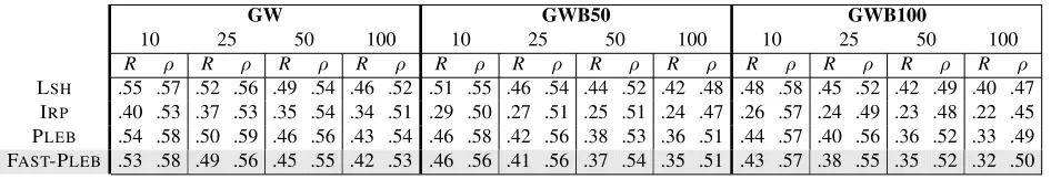
GW GWB50 GWB100

10 25 50 100 10 25 50 100 10 25 50 100

R ρ R ρ R ρ R ρ R ρ R ρ R ρ R ρ R ρ R ρ R ρ R ρ

LSH .55 .57 .52 .56 .49 .54 .46 .52 .51 .55 .46 .54 .44 .52 .42 .48 .48 .58 .45 .52 .42 .49 .40 .47 IRP .40 .53 .37 .53 .35 .54 .34 .51 .29 .50 .27 .51 .25 .51 .24 .47 .26 .57 .24 .49 .23 .48 .22 .45 PLEB .54 .58 .50 .59 .46 .56 .43 .54 .46 .58 .42 .56 .38 .53 .36 .51 .44 .57 .40 .56 .36 .52 .33 .49 FAST-PLEB .53 .58 .49 .56 .45 .55 .42 .53 .46 .56 .41 .56 .37 .54 .35 .51 .43 .57 .38 .55 .35 .52 .32 .50

Table 5: Evaluation results on comparing LSH, IRP, PLEB, and FAST-PLEBwithk= 3000,b= 40,p= 1000andq= 10with exact nearest neighbors across three different data sets:GW,GWB50, andGWB100. We report results on recall (R) andρmetric. The gray color row is the system that we use for further evaluations.

nearest neighbors that are found in both the lists and then Pearson’s (ρ) correlation captures if the rela-tive order of these lists is preserved in both the sim-ilarity lists. We also compute R and ρ at various

l={10,25,50,100}.

Results: For the first experiment, we evaluate IRP, PLEB, and FAST-PLEBagainst the exact

near-est neighbor similarity lists. For IRP, we sample first p rows and only use p rather than k, this en-sures that all the three methods (IRP, PLEB, and

FAST-PLEB) take the same query time. We vary the approximate nearest neighbor beam parameter

b = {20,30,40,50,100} that controls the number of closest neighbors for a word with respect to each independent random projection. Note, with increas-ingb, our algorithm approaches towards LSH

(com-puting Hamming distance with respect to all the words). For FAST-PLEB, we setq = 10(q << k) that is the number of random bits selected out ofkto generateppermuted bit vectors of sizeq. The results are reported in Table 3, where the first row com-pares the LSH approach against the exact

similar-ity list for test set words. Across three columns we compare IRP, PLEB, and FAST-PLEB. For all meth-ods, increasing b means better recall. If we move down the table, withb= 100, IRP, PLEB, and FAST

-PLEBget results comparable to LSH(reaches an up-per bound). However, using largeb implies gener-ating a long potential nearest neighbor list close to the size of the unique context vectors. If we focus on the gray color row withb = 40(This will have comparativelysmallpotential list and return nearest neighbors in less time), IRP has worse recall with best pre-processing time. FAST-PLEB (q = 10) is comparable to PLEB(using all bitsq = 3000) with pre-processing time300times faster than PLEB. For rest of this work,FLAGwill use FAST-PLEB as it has best recall and pre-processing time with fixed

b= 40.

For the second experiment, we vary parameter

q = {1,5,10,100,3000} for FAST-PLEB in Table

4. Table 4 demonstrates usingq = {1,5} result in worse recall, however usingq = 5 for FAST-PLEB

is better than IRP. q = 10 has comparable recall toq = {100,3000}. For rest of this work, we fix

q= 10as it has best recall and pre-processing time. For the third experiment, we increase the size of the data set across the Table 5. With the increase in size of the data set, LSH, IRP, PLEB, and FAST

-PLEB (q = 10) have worse recall. The reason for

jazz yale soccer physics wednesday

reggae harvard basketball chemistry tuesday rockabilly cornell hockey mathematics thursday rock fordham lacrosse biology monday bluegrass rutgers handball biochemistry friday

indie dartmouth badminton science saturday baroque nyu softball microbiology sunday

ska ucla football geophysics yesterday funk princeton tennis economics tues banjo stanford wrestling psychology october blues loyola rugby neuroscience week

Table 6:Sample Top10similarity lists returned by FAST-PLEB

withk= 3000,p= 1000,b= 40andq= 10fromGWB100.

three data sets, FAST-PLEBhas recall comparable to PLEB with best pre-processing time. Hence, for the

next evaluation to show the quality of final lists we use FAST-PLEBwithq = 10forGWB100data set.

In Table 6, we list the top10most similar words for some words found by our system FLAGusing

GWB100data set. Even though FLAG’s approxi-mate nearest neighbor algorithm has less recall with respect to exact but still the quality of these nearest neighbor lists is excellent.

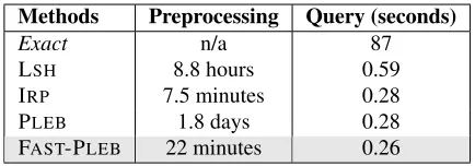
For the final experiment, we demonstrate the pre-processing and query time results comparing LSH, IRP, PLEB, and FAST-PLEB with k = 3000, p =

1000, b = 40andq = 10 parameter settings. For

pre-processing timing results, we perform all the ex-periments (averaged over5runs) onGWB100data set with 106, 733 words. The second pre-processing step of the system FLAG (Section 3.2) that is di-mensionality reduction from RD to Rk took 8.8

hours. The pre-processing time differences among IRP, PLEB, and FAST-PLEBfrom third step (Section 3.3) are shown in second column of Table 7. Ex-perimental results show that the naive baseline IRP

is the fastest and FAST-PLEB has120 times faster pre-processing timecompared to PLEB.

For comparing query time among several meth-ods, we evaluate over447words (Section 4.2). We report average timing results (averaged over10runs and447words) to find top100nearest neighbors for single query word. The results are shown in third column of Table 7. Comparing first and second rows show that LSH is 87 times faster than computing exact top-100(cosine similarity) nearest neighbors. Comparing second, third, fourth and fifth rows of the table demonstrate that IRP, PLEB and FAST-PLEB

Methods Preprocessing Query (seconds)

Exact n/a 87

LSH 8.8 hours 0.59

IRP 7.5 minutes 0.28

PLEB 1.8 days 0.28

FAST-PLEB 22 minutes 0.26

Table 7: Preprocessing and query time results compar-ing exact, LSH, IRP, PLEB, and FAST-PLEBmethods on GWB100data set.

Language english chinese japanese spanish russian

Place africa america washington london pacific

Nationality american european french british western

Date january may december october june

Organization ford microsoft sony disneyland google

Table 8: Query terms for Google Sets Problem evaluation

methods are twice as fast as LSH.

5 Applications

We use the graph constructed by FLAG from

GWB100 data set (110 GB) by applying FAST -PLEBwith parametersk= 3000,p= 1000,q= 10

andb= 40. The graph has106,733nodes (words),

with each node having100edges that denote the top

l = 100approximate nearest neighbors associated

with each node. However, FLAG applied FAST

-PLEB (approximate search) to find these neighbors. Therefore many of these edges can be noisy for our applications. Hence for each node, we only consider top10edges. In general for graph-based NLP prob-lems; for example, constructing web-derived polar-ity lexicons (Velikovich et al., 2010), top25 edges were used, and for unsupervised part-of-speech tag-ging using label propagation (Das and Petrov, 2011), top5edges were used.

5.1 Google Sets Problem

Language:german, french, estonian, hungarian, bulgarian

Place:scandinavia, mongolia, mozambique, zambia, namibia

Nationality:german, hungarian, estonian, latvian, lithuanian

Date:september, february, august, july, november

Organization:looksmart, hotbot, lycos, webcrawler, alltheweb

Table 9: Learned terms for Google Sets Problem

Concrete car, house, tree, horse, animal seeds man, table, bottle, woman, computer Abstract idea, bravery, deceit, trust, dedication

seeds anger, humour, luck, inflation, honesty

Table 10: Example seeds for bootstrapping.

We conduct a manual evaluation to directly mea-sure the quality of returned words. We recruited1 annotator and developed annotation guidelines that instructed each recruiter to judge whether learned values are similar to query words or not. Overall the annotator found almost all the learned words to be similar to the query words. However, the algorithm can not differentiate between different senses of the word. For example, “French” can be a language and a nationality. Table 9 shows the top ranked words with respect to query words.

5.2 Learning Concrete and Abstract Words

Our goal is to automatically learn concrete and ab-stract words (Turney et al., 2011). We apply boot-strapping (Kozareva et al., 2008) on the word graphs by manually selecting10seeds for concrete and ab-stract words (see Table 10). We use in-degree (sum of weights of incoming edges) to compute the score for each node which has connections with known (seeds) or automatically labeled nodes, previously exploited to learn hyponymy relations from the web (Kozareva et al., 2008). We learn concrete and ab-stract words together (known as mutual exclusion principle in bootstrapping (Thelen and Riloff, 2002; McIntosh and Curran, 2008)), and each word is as-signed to only one class. Moreover, after each it-eration, we harmonically decrease the weight of the in-degree associated with instances learned in later iterations. We add 25 new instances at each itera-tion and ran100iterations of bootstrapping, yielding 2506 concrete nouns and2498 abstract nouns. To evaluate our learned words, we searched in WordNet whether they had ‘abstraction’ or ’physical’ as their hypernym. Out of 2506 learned concrete nouns,

Concrete: girl, person, bottles, wife, gentleman, mi-crocomputer, neighbor, boy, foreigner, housewives, texan, granny, bartender, tables, policeman, chubby, mature, trees, mainframe, backbone, truck

Abstract: perseverance, tenacity, sincerity, profes-sionalism, generosity, heroism, compassion, commit-ment, openness, resentcommit-ment, treachery, deception, no-tion, jealousy, loathing, hurry, valour

Table 11: Learned concrete/abstract words.

1655were found in WordNet. According to Word-Net, 74% of those are concrete and 26% are ab-stract. Out of2498learned abstract nouns,942were found in WordNet. According to WordNet, 5%of those are concrete and95%areabstract. Table 11 shows the top ranked concrete and abstract words.

6 Conclusion

We proposed a system, FLAG which constructs

fast large-scale approximate graphs from large data sets. To build this system we proposed a distributed online-PMI algorithm that scaled up to 110GB of web data with 866million sentences in less than 2 days using100quad-core nodes. Our both intrinsic and extrinsic experiments demonstrated that online-PMI algorithm not at all loses globally good con-texts and perform comparable to offline-PMI. Next, we proposed FAST-PLEB (a variant of PLEB) and empirically demonstrated that it has recall compa-rable to PLEB with120times faster pre-processing time. Finally, we show the applicability ofFLAGon two applications: Google-Sets problem and learning concrete and abstract words.

In future, we will applyFLAGto construct graphs using several kinds of contexts like lexical, seman-tic, syntactic and dependency relations or a combi-nation of them. Moreover, we will apply graph theo-retic models on graphs constructed usingFLAGfor solving a large variety of NLP applications.

Acknowledgments

This work was partially supported by NSF Award

IIS-1139909. Thanks to Graham Cormode and

References

Dimitris Achlioptas. 2003. Database-friendly random projections: Johnson-lindenstrauss with binary coins.

J. Comput. Syst. Sci., 66(4):671–687.

Eneko Agirre, Enrique Alfonseca, Keith Hall, Jana Kravalova, Marius Pas¸ca, and Aitor Soroa. 2009. A study on similarity and relatedness using distributional and wordnet-based approaches. InNAACL ’09: Pro-ceedings of HLT-NAACL.

Moses Charikar, Kevin Chen, and Martin Farach-Colton. 2004. Finding frequent items in data streams. Theor. Comput. Sci., 312:3–15, January.

Moses S. Charikar. 2002. Similarity estimation tech-niques from rounding algorithms. InIn Proc. of 34th STOC, pages 380–388. ACM.

K. Church and P. Hanks. 1989. Word Associa-tion Norms, Mutual InformaAssocia-tion and Lexicography. In Proceedings of ACL, pages 76–83, Vancouver, Canada, June.

Graham Cormode and Marios Hadjieleftheriou. 2008. Finding frequent items in data streams. InVLDB. Graham Cormode and S. Muthukrishnan. 2004. An

im-proved data stream summary: The count-min sketch and its applications. J. Algorithms.

Dipanjan Das and Slav Petrov. 2011. Unsupervised part-of-speech tagging with bilingual graph-based pro-jections. In Proceedings of the 49th Annual Meet-ing of the Association for Computational LMeet-inguistics: Human Language Technologies, pages 600–609, Port-land, Oregon, USA, June. Association for Computa-tional Linguistics.

Cristian Estan and George Varghese. 2002. New di-rections in traffic measurement and accounting. SIG-COMM Comput. Commun. Rev., 32(4).

L. Finkelstein, E. Gabrilovich, Y. Matias, E. Rivlin, Z. Solan, G. Wolfman, and E. Ruppin. 2002. Plac-ing search in context: The concept revisited. InACM Transactions on Information Systems.

Zoubin Ghahramani and Katherine A. Heller. 2005. Bayesian Sets. Inin Advances in Neural Information Processing Systems, volume 18.

Amit Goyal and Hal Daum´e III. 2011. Approximate scalable bounded space sketch for large data NLP. In

Empirical Methods in Natural Language Processing (EMNLP).

Amit Goyal, Hal Daum´e III, and Suresh Venkatasubra-manian. 2009. Streaming for large scale NLP: Lan-guage modeling. InNAACL.

Amit Goyal, Graham Cormode, and Hal Daum´e III. 2012. Sketch algorithms for estimating point queries in NLP. In Empirical Methods in Natural Language Processing (EMNLP).

D. Graff. 2003. English Gigaword. Linguistic Data Con-sortium, Philadelphia, PA, January.

Piotr Indyk and Rajeev Motwani. 1998. Approximate nearest neighbors: towards removing the curse of di-mensionality. In Proceedings of the thirtieth annual ACM symposium on Theory of computing, STOC ’98, pages 604–613. ACM.

Zornitsa Kozareva, Ellen Riloff, and Eduard Hovy. 2008. Semantic class learning from the web with hyponym pattern linkage graphs. In Proceedings of ACL-08: HLT, pages 1048–1056, Columbus, Ohio, June. As-sociation for Computational Linguistics.

Abby Levenberg, Chris Callison-Burch, and Miles Os-borne. 2010. Stream-based translation models for statistical machine translation. In Human Language Technologies: The 2010 Annual Conference of the North American Chapter of the Association for Com-putational Linguistics, HLT ’10, pages 394–402. As-sociation for Computational Linguistics.

Ping Li, Trevor J. Hastie, and Kenneth W. Church. 2006. Very sparse random projections. In Proceedings of the 12th ACM SIGKDD international conference on Knowledge discovery and data mining, KDD ’06, pages 287–296. ACM.

Ping Li, Kenneth Ward Church, and Trevor Hastie. 2008. One sketch for all: Theory and application of condi-tional random sampling. InNeural Information Pro-cessing Systems, pages 953–960.

Tara McIntosh and James R Curran. 2008. Weighted mutual exclusion bootstrapping for domain indepen-dent lexicon and template acquisition. InProceedings of the Australasian Language Technology Association Workshop 2008, pages 97–105, December.

G.A. Miller and W.G. Charles. 1991. Contextual corre-lates of semantic similarity. Language and Cognitive Processes, 6(1):1–28.

Patrick Pantel, Eric Crestan, Arkady Borkovsky, Ana-Maria Popescu, and Vishnu Vyas. 2009. Web-scale distributional similarity and entity set expansion. In

Proceedings of EMNLP.

Delip Rao and Deepak Ravichandran. 2009. Semi-supervised polarity lexicon induction. InProceedings of the 12th Conference of the European Chapter of the ACL (EACL 2009), pages 675–682, Athens, Greece, March. Association for Computational Linguistics. Deepak Ravichandran, Patrick Pantel, and Eduard Hovy.

2005. Randomized algorithms and nlp: using locality sensitive hash function for high speed noun clustering. InProceedings of ACL.

H. Rubenstein and J.B. Goodenough. 1965. Contextual correlates of synonymy. Computational Linguistics, 8:627–633.

M. Thelen and E. Riloff. 2002. A Bootstrapping Method for Learning Semantic Lexicons Using Extraction Pat-tern Contexts. InProceedings of the Empirical Meth-ods in Natural Language Processing, pages 214–221. Peter D. Turney and Patrick Pantel. 2010. From

fre-quency to meaning: Vector space models of seman-tics. JOURNAL OF ARTIFICIAL INTELLIGENCE RESEARCH, 37:141.

Peter Turney, Yair Neuman, Dan Assaf, and Yohai Co-hen. 2011. Literal and metaphorical sense identifi-cation through concrete and abstract context. In Pro-ceedings of the 2011 Conference on Empirical Meth-ods in Natural Language Processing, pages 680–690. Association for Computational Linguistics.

Benjamin Van Durme and Ashwin Lall. 2009a. Prob-abilistic counting with randomized storage. In IJ-CAI’09: Proceedings of the 21st international jont conference on Artifical intelligence.

Benjamin Van Durme and Ashwin Lall. 2009b. Stream-ing pointwise mutual information. In Advances in Neural Information Processing Systems 22.

Benjamin Van Durme and Ashwin Lall. 2010. Online generation of locality sensitive hash signatures. In

Proceedings of the ACL 2010 Conference Short Pa-pers, pages 231–235, July.

Benjamin Van Durme and Ashwin Lall. 2011. Efficient online locality sensitive hashing via reservoir count-ing. InProceedings of the ACL 2011 Conference Short Papers, June.

Leonid Velikovich, Sasha Blair-Goldensohn, Kerry Han-nan, and Ryan McDonald. 2010. The viability of web-derived polarity lexicons. InHuman Language Tech-nologies: The 2010 Annual Conference of the North American Chapter of the Association for Computa-tional Linguistics, pages 777–785, Los Angeles, Cal-ifornia, June. Association for Computational Linguis-tics.