A New Clustering Algorithm On Nominal Data Sets
Bin Wang
Abstract—This paper presents a new clustering technique named as the Olary algorithm, which is suitable to cluster nominal data sets. This algorithm uses a new code with the name of the Olary code to transform nominal attributes into integer ones through a process named as the Olary transformation. The number of integer attributes we get through the Olary transformation is usually different from that of the original nominal attributes. Meanwhile, an extension of the Olary algorithm, which we call the ex-Olary algorithm, is introduced. Furthermore, we provide a useful way to estimate the number of underlying clusters by the use of a new kind of diagram, which is called Number of Clusters versus Distance Diagram (NCDD for short).
Index Terms-Clustering, nominal, the Olary code, the Olary transformation, the ex-Olary algorithm, NCDD
I. INTRODUCTION
Advances in communication systems and high performance computers enable us to easily collect valuable information from the Internet and to construct databases that store huge amount of information [1]. As a result, data mining has becoming more and more popular and important in the past decades. Among various kinds of technologies in the area of data mining, clu-stering has received considerable attention.
Different from the classification technique, clustering is an un-supervised learning method in the purpose of discovering the underlying patterns and structures of a given data set. To-day, there are many kinds of clustering algorithms and there are mainly five categories [2]: hierarchical clustering, partitioned clustering, density-based clustering, grid-based clustering and model-based clustering. Specially, in partitioned clustering, ea-ch cluster is represented by its center point.
The application of clustering algorithms to scientific res-earch faces many challenges. First, almost all the algorithms require pre-specified parameters, such as the number of clusters k, a small positive real number
δ
that is useful when testing the terminal conditions, a positive integer seed and so on. Second, different data sets contain different types of data points as well as different underlying structures. Usually it is not an easy job to select the most suitable clustering algorithm for a given data set without priori knowledge. Third, most clustering algorithms are only suitable for numeric data sets. However, in practical applications, we face a lot of nominal data sets.In this paper we provide a new clustering algorithm named as the Olary algorithm, which can be used to cluster nominal data sets. Besides, we will discuss a useful method to estimate the number of underlying clusters by the use of the NCDD. The
Manuscript received December 26, 2009.
Bin Wang is with the Institute of Telecommunications, Xi’an Jiaotong University, Xi’an, 710049, China (email: [email protected])
remaining parts are arranged as follows. In section two, we will introduce a new code with the name of the Olary code, which is used to transform nominal attributes into binary integer ones. In section three we will discuss how to compute the distance between two data points by the use of the Olary transformation. Section four contains the running process of the Olary algori-thm in detail, and section five gives some experiments to show the performance of the Olary algorithm. Section six suggests an extension of the Olary algorithm, which is called the ex-Olary algorithm. What’s more, a useful way of estimating the number of underlying clusters by the use of the NCDD will be disc-ussed. Finally, in section seven, we draw conclusions and sug-gest some possible directions for further researches.
II. THE OLARY CODE
In this section we will introduce a new code named as the Olary code. First, let’s see some examples. The 1-length Olary code has two different values, 1 and 0. The 2-length Olary code has three different values, which are 10, 11 and 01. The 3-length Olary code has four different values and they are 101, 100, 110 and 010, respectively.
Now we can present the definition of the Olary code as fol-lows. Assume k is a positive integer (k=1, 2, 3…). The k-length Olary code has k+1 different values and all the values are bin-ary integer sequences. We can get these values in the following manner. If k is odd, the first value is 1010…101. Else if k is even, the first value is 1010…1010. We can see that the first value contains k binary integer numbers and the first number is always 1. Here 1 is the opposite number of 0 and vice versa. Replacing the k-th number of the first value with its opposite number, we receive the second value of the k-length Olary code. Turning the (k-1)-th number of the second value into its opposite number, we get hold of the third value of the k-length Olary code. In a word, when i is larger than one, we gain the i-th value of i-the k-lengi-th Olary code just by replacing i-the (k-i+2)-th number of the (i-1)-th value with its opposite number.
The Olary code can be considered as a coding system. The k-length Olary code has (k+1) different values. From the way of getting the (k+1) values of the k-length Olary code, we know there is exactly one different number between the i-th value and the (i+1)-th value (i=1…k). As a special case, turning all the numbers of the first value into their opposite numbers, we get the (k+1)-th value of the k-length Olary code.
III. THE DISTANCE METRIC
takes 1 or 0 as its value. Usually the number of integer attri-butes is different from that of the original nominal ones. And in some cases it changes greatly. In the following, we will discuss the process of this transformation, which we call the Olary tra-nsformation.
We use the (k-1)-length Olary code to transform a nominal attribute with k different values, because the (k-1)-length Olary code has exactly k different values. For example, suppose an attribute with the name of legsNumber has four different values
and they are two legs, four legs, six legs and eight legs,
res-pectively. So we should use the 3-length Olary code to do the transformation. First, randomly push the four different values of the nominal attribute legsNumber into a stack named as stack1. Second, randomly push the four values of the 3-length
Olary code into another stack with the name of stack2. Third,
pop the top value v1 of stack1 and pop the top value v2 of stack2. Use v2 to substitute v1. Repeat the third step until both
the two stacks are empty. By now, the Olary transformation on the attribute legsNumber is finished. This single nominal
attri-bute has been transformed into three integer ones, each of whi-ch takes 1 or 0 as its value.
Now we can give the distance metric used in the Olary algorithm. Consider two data points named as p1 and p2,
res-pectively. Perform the Olary transformation on the two points. Assume m is the number of integer attributes each of the two points has after the Olary transformation. Here p1.value(i) is
used to denote the value of the i-th integer attribute of p1. And p2.value(i) is the value of the i-th integer attribute of p2. Then
we can compute the distance between p1 and p2 as follows.
for i = 1 to m
if p1.value(i) ≠ p2.value(i)
distance = distance + 1; end if
end for
return distance;
IV. THE OLARY ALGORITHM
In this section we will discuss the Olary algorithm, whose main mechanism is the same as the simple K-means. The two algorithms have different ways of calculating the “distance” between two data points. The simple K-means uses the Euclidean distance as shown in (1). Here l is the number of dimensions of x and y. However, in the Olary algorithm, we c-
∑
=
−
=
−
li
i
i
y
x
y
x
1
2
2
(
)
||
||
. (1)hoose a new distance metric as discussed in section three. The running process of the Olary algorithm is shown as the follo-wing steps.
STEP1. Transform all the data points in the original data set through the process of the Olary transformation. We get hold of a new data set named as instances, which contains only
binary integer attributes.
STEP2. Initialize relative parameters, including the number of clusters k and a positive integer seed. What’s more, initialize
a third parameter named as maxIterations, which is also a
positive integer and denotes the maximum number of iterations before the Olary algorithm terminates.
STEP3. Use the function initCenters(instances, k, seed) as
shown in Fig. 1 to finish the initialization of the k center points. Here we use two integer arrays centers1[k][] and centers2[k][]
to store the center points.
STEP4. Compute the distances from each point in the data set instances to the current k center points. If the current point
has the smallest distance from the i-th center point, then assign it to the i-th cluster. Use an array named as index[] to store the
clustering indexes of all the points in instances.
STEP5. Copy all the elements of the array centers1[k][]
into centers2[k][]. Then compute the k new center points
acco-rding to the process computeCenters(instances, index[], k) as
shown in Fig. 2. Store the k new centers into centers1[k][].
STEP6. If the contents of the two arrays centers1[k][] and centers2[k][] are the same or maxIterations is smaller than the
[image:2.595.306.550.398.598.2]current number of iterations, the Olary algorithm stops. Else go back to STEP4 and continue the iteration.
Figure 1. function initCenters(instances, k, seed)
V. EXPERIMENTS
In this section we illustrate the performance of the Olary algorithm described in the previous sections. All the data sets used here are from the UCI data set repository.
The first one is the zoo data set, which has 16 attributes, including 15 ones and an integer one. The integer attribute
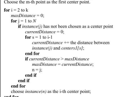
Here we use Nto denote the number of data points. And instance(i) is the i-th point. What’s more, centers1[i] is the
center point of the i-th cluster. Assume m equals to seed.
Choose the m-th point as the first center point. for i = 2 to k
maxDistance = 0;
for j = 1 to N
if instance(j) has not been chosen as a center point
currentDistance = 0;
for s = 1 to i-1
currentDistance += the distance between
instance(j) and centers1[s];
end for
if currentDistance > maxDistance
maxDistance = currentDistance;
n = j; end if end if end for
choose instance(n) as the i-th center point;
suggests the number of legs, with three integer values: 0, 2 and 4. So here we consider it as a nominal attribute. We selected 74 data points from the zoo data set to form a new set with the name of zoo1. The zoo1 data set contains three clusters and its underlying structure is shown in Tab. I.
In the Olary algorithm, the random property of the Olary transformation means one nominal data set can be transformed into many different integer ones. Does this property have great influence on the final clustering result? From the results sho-wn in Tab. II we draw the conclusion that the Olary algorithm gains very good results on the zoo1 data set and the random property of the Olary transformation has little influence on the
[image:3.595.45.289.552.643.2]Figure 2. the process computeCenters(instances, index[], k)
TABLE I. THE UNDERLYING STRUCTURE OF THE ZOO1 DATA SET
cluster ID IDs of data points
1
1,2,4,5,6,7,10,11,15,17,20,22,23,24,25, 26,29,30,35,36,37,38,39,40,41,42,49,50,
51,52,53,54,55,56,59,60,65,69,70,72,73
2 3,8,9,13,16,28,32,47,48,58,63,66,68 3 12,14,18,19,21,27,31,33,34,
43,44,45,46,57,61,62,64,67,71,74
final result. What’s more, considering the single integer attri-bute in the zoo1 data set as a nominal one is suitable here.
Here is another question. Can we gain satisfactory cluster-ing results by randomly initializcluster-ing the center points instead of using the function initCenters(instances, k, seed)? In one expe-
riment, we initialized the centers by the use of three randomly
selected points from the data set and the corresponding result is shown in Tab. III. With the help of the underlying structure, we know this result is not acceptable at all. So we draw the conclusion that the function initCenters(instances, k, seed) is
of great importance to gain good clustering results.
The second data set is the sponge data set, which contains 42 nominal attributes and 3 integer ones. Two of the 3 integer attributes have five values: 0, 1, 2, 3 and 4. And the third one
TABLE II. RESULTS OF DIFFERENT TRANSFORMATIONS
transformation correct rate
trans I(0→10, 2→11, 4→01) 97.3%
trans I(0→10, 2→01, 4→11) 100%
trans I(0→11, 2→10, 4→01) 100%
trans II(0→10, 2→11, 4→01) 97.3%
TABLE III. RESULT GAINED BY RANDOMLY INITIALIZING CENTERS
cluster ID IDs of data points
1 2,6,7,10,15,20,22,23,25,26,29,30, 42,51,56,65,69,70,72
2
1,4,5,11,17,24,35,36,37,38,39,40, 41,49,50,52,53,54,55,59,60,73
3
3,8,9,12,13,14,16,18,19,21,27,28,31,32, 33,34,43,44,45,46,47,48,57,58,61,62,
63,64,66,67,68,71,74
TABLE IV. THE UNDERLYING STRUCTURE OF THE SPONGE1 DATA SET
cluster ID IDs of the data points
1 2,3,4,5,6,7,8,9,38,39 2 1,37,40,45,46,48,49 3 12,13,14,15,16,17,18,19,20,21,
22,23,24,25,29,36
4 10,11,26,27,28,30,31,32,33,34, 35,41,42,43,44,47
TABLE V. RESULTS OF TWO DIFFERENT TRANSFORMATIONS
transformation correct rate
trans I 89.8%
trans II 93.9%
has four values: 0, 1, 2 and 3. Here we also consider them as nominal attributes. Many of the attributes in the sponge data set have a lot of values. Moreover, this data set has a high dimensionality. So the sponge data set is much more complex than the zoo data set. We selected 49 points to form a new set with the name of sponge1. The underlying clustering structure of sponge1 is shown in Tab. Ⅳ. After the Olary transfor-mation, each point has 96 binary integer attributes, while each point has only 45 attributes in the original sponge data set. In other words, the number of attributes changes greatly.
Now we examine whether the random property of the Olary transformation is suitable when using the Olary algori-thm to cluster the sponge1 data set. From the results shown in Tab. V we draw the conclusion that the Olary algorithm gains Here we assume the number of attributes is m. And we use
instances(s).value(j) to denote the value of the j-th
attri-bute of the s-th data point. N is the number of data points. for i = 1 to k (k is the user-specified number of clusters) for j = 1 to m
count0 = 0; count1 = 0; for s = 1 to N if index[s]==i
if instances(s).value(j)==0
count0 ++; else
count1 ++; end if
end if end for
if count0 >= count1 centers1[i][j] = 0;
else
centers1[i][j] = 1; end for
very good results on the sponge1 data set and the difference between the two results gained on two different integer data sets due to the random property of the Olary transformation is very small, although the sponge1 data set is rather complex. As a result, we draw the conclusion that the random property of the Olary transformation is suitable when using the Olary algorithm to cluster the sponge1 data set. What’s more, exper-iments show that the random property of the Olary transfor-mation is also suitable for transforming the 3 integer attributes, which are considered as nominal ones.
TABLE VI. RESULT GAINED BY RANDOMLY INITIALIZED CENTERS
cluster ID IDs of data points
1 2,3,4,5,6,7,8,9,10,11,26,27,28,30,31,32, 33,34,35,38,39,41,42,43,44,47
2 12,13,14,15,16,18,19,20,22,23,24,25,36 3 29 4 1,17,21,37,40,45,46,48,49
Figure 3. the calculation of sumDistance
TABLE VII. RESULTS OF THE OLARY ALGORITHM ON SPONGE1
IDs of initial center points correct rate
28,41,1,13 87.8% 27,28,1,17 81.6% 9,17,1,14 83.7%
In one experiment we randomly initialized the center points and the result is shown in Tab. VI. Looking back at the underlying structure of the sponge1 data set in Tab. IV, we come to the point that the clustering result in Tab. VI is not acceptable at all. This reflects the importance of the process
initCenters(instances, k, seed), which is used to initialize all
the center points when we use the Olary algorithm to cluster a given data set.
VI. ESTIMATE THE NUMBER OF UNDERLYING CLUSTERS In this section we introduce an extension of the Olary algo-rithm. Meanwhile, we provide a useful way of estimating the number of underlying clusters by the use of the NCDD. We have discussed some relative theories in [3]. However, the method we introduce here is different from that in [3].
A. the ex-Olary algorithm
We gain the following information after running the Olary algorithm:
• The center points of the resulting clusters are stored in the array centers1[k][], and here k is the user-specified
number of clusters.
• The array named as index[N] stores the clustering
index of each point, and here N is the number of points in the original data set.
Now we introduce a new parameter named as sumDistance,
the calculation of which is shown in Fig. 3. We can see the value of sumDistance is the sum of the distances from each
point to the corresponding center point.
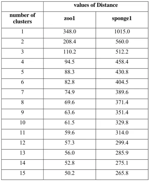
TABLE VIII. VALUES OF SUMDISTANCE
values of Distance
number of
clusters zoo1 sponge1
1 348.0 1015.0
2 208.4 560.0
3 110.2 512.2
4 94.5 458.4
5 88.3 430.8
6 82.8 404.5
7 74.9 389.6
8 69.6 371.4
9 63.6 351.4
10 61.5 329.8
11 59.6 314.0
12 57.3 299.4
13 56.0 285.9
14 52.8 275.1
15 50.2 265.8
The value of sumDistance changes as the clustering result
varies. And we gain different results when the user-specified number of clusters k changes. So the value of sumDistance
changes as k changes. Furthermore, for a fixed value of k, we can still get different results if the initialization of the k centers differs, although there is usually little difference as long as the results are acceptable. Thus, sumDistance usually changes as
the initial k center points vary. We introduce an extension of the Olary algorithm as shown in Fig. 4, and we call it the ex-Olary algorithm. From Fig. 4 we know the ex-ex-Olary algorithm tends to gain a global minimum of sumDistance for a fixed
value of k. Assume that N is the number of points. We can get N values of sumDistance by setting the parameter seed to be
each ID of the N data points, corresponding to N clustering for i = 1 to N
dis = the distance between the i-th point and the
corresponding center point centers1[index[i]];
sumDistance = sumDistance + dis;
end for
[image:4.595.43.293.214.503.2] [image:4.595.304.553.271.576.2]results. And the smallest one of the N values is the global minimum that the ex-Oary algorithm tries to get. Just randomly choose one result as the final result if the global minimum corresponds to several initializations and clustering results.
Setting k to be 3, we run the ex-Olary algorithm to cluster the zoo1 data set. The data set after the Olary transformation is the same as trans I in Tab. II. Corresponding to the global minimum of sumDistance, the correct rate of the clustering
result is 97.3%, while the correct rate of the result in Tab. II is also 97.3%. Now let’s turn to the sponge1 data set, which is rather complex. The data set used here after the Olary trans-formation is the same as trans I in Tab. V. We did several exp-eriments on this data set by the use of the Olary algorithm and the results are shown in Tab. VII. The correct clustering rate by the use of the ex-Olary algorithm is 87.8%, which is the same as the best one in Tab. VII. By now, we can draw a conclusion that the clustering result of the ex-Olary algorithm is close to the best result that the Olary algorithm can gain. What’s more, the distance metric we use is just to count the number of integer attributes having different values between data points after the Olary transformation. As a result, the running time of the ex-Olary algorithm is usually acceptable.
Figure 4. the ex-Olary algorithm
B. Estimate the Number of Clusters by the Use of the NCDD
In order to estimate the number of underlying clusters in a given data set, we introduce a new variable Distance, the
calculation of which is shown in Fig. 5. The ex-Olary algorithm tries to get the global minimum of the parameter sumDistance.
Here the global minimum means the smallest value of the N values of sumDistance got by running the Olary algorithm N
times, each time setting seed to be a different ID of the N
points in the data set. However, the value of the new variable
Distance is the average of the N values of sumDistance. The
variable Distance is a better estimate of the sum of the
dis-tances from each point to the corresponding center point than
sumDistance. Then a new kind of diagram can be drawn. The
horizontal axis of the diagram is the number of user-specified
number of clusters, and the vertical axis is the corresponding values of the parameter Distance. We call this kind of diagram
Number of Clusters versus Distance Diagram, NCDD for short. In the following, we will estimate the number of underlying clusters by the use of NCDD along with similar theories having been discussed in [3].
For both the zoo1 and the sponge1 data sets, the values of
Distance are shown in Tab. VIII. The NCDD for the zoo1 data
set is shown in Fig. 6. Here k is the user-specified number of clusters and m is the number of underlying clusters. When k is smaller than m, at least one resulting cluster contains more than one underlying clusters. The distances between data points from different clusters are usually much larger than those of points from the same cluster. So values of Distance are very
large. As k increases, resulting clusters consisting of more than one underlying clusters split and the values of Distance usually
decrease sharply. When k is smaller than 3, the value of
Distance decreases significantly as k increases in Fig. 6.
When k is larger than m, each resulting cluster contains at most one underlying cluster. So the value of Distance is usually
small. What’s more, some underlying clusters split as k increases. The value of Distance decreases more and more
slowly as k increases, basing on the fact that distances between data points in the same cluster differ little. In other words, the value of Distance tends to converge. As shown in Fig. 6, when
k is larger than 3, Distance tends to converge as k increases.
Figure 5. the caculation of Distance
When k equals to m-1, there is exactly one resulting cluster that contains two underlying clusters. As k increases to m, this resulting cluster splits. As a result, the value of Distance
usually decreases significantly. When k is m+1, one underlying cluster will split into two sub-clusters. The value of the decre-ase of Distance is usually small, because data points in the
same cluster are quite similar to each other. As a result, we can draw the conclusion that the value of |value(m-1) – value (m)| is usually much larger than that of |value(m) – value(m+1)|, where value(i) denotes the value of Distance when k equals to i.
This is a significant property, which is of great importance when estimating the number of underlying clusters. In Fig. 6, |value(2) – value(3)| is much larger than |value(3) – value(4)|, indicating that the correct number of underlying clusters is 3. Furthermore, a resulting NCDD similar to that in Fig. 6 sugg-ests good clustering results, and vice versa.
Here we use N to denote the number of points in the original data set.
minValue = 0.0; minSeed = 0;
for i = 1 to N seed = i;
run the Olary algorithm;
compute the value of sumDistance as shown in Fig. 3;
if minValue > sumDistance
minValue = sumDistance;
minSeed = i;
end if end for
now we know setting seed to be minSeed, we can get the
global minimum of sumDistance by the use of the Olary
algorithm;
Here we use N to denote the number of points in the original data set.
for i = 1 to N seed = i;
run the Olary algorithm;
compute the value of sumDistance as shown in Fig. 3;
Distance = Distance + sumDistance;
end if end for
Distance = Distance/N;
Now let’s turn to the NCDD of the sponge1 data set shown in Fig. 7. This diagram seems not as good as that in Fig. 6, suggesting that the clustering results are not as satisfactory as those on the zoo1 data set. However, the results are acceptable, and we can estimate the correct number of underlying clusters as follows. When k is smaller than 4, the value of Distance
decreases sharply as k increases. When k is larger than 4, the
Distance decreases more slowly as k increases. What’s more,
[image:6.595.41.289.251.438.2]the value of |value(3) – value(4)| is significantly larger than the value of |value(4) – value(5)|, which is the important property at the point of k being equal to the correct number of under-lying clusters. Basing on theses facts, we can draw the conclusion that the number of underlying clusters in the sponge1 data set is 4, which is the correct number in fact.
Figure 6. the NCDD of the zoo1 data set
VII. CONCLUSIONS
In this paper we give a discussion of the Olary algorithm, which is suitable to cluster nominal data sets. A new code with the name of the Olary code is introduced. And nominal attr-ibutes can be transformed into binary integer ones through the process of the Olary transformation. The number of integer attributes is usually different from that of the nominal ones. For example, the sponge1 data set has 96 integer attributes after the Olary transformation, while the number of the original attri-butes is only 45. Experiments show that the Olary algorithm has good performances on nominal data sets, including high-dimensional ones such as the sponge1 data set. What’s more, the random property of the Olary transformation is suitable.
The ex-Olary algorithm, which is an extension of the Olary algorithm, tries to find the global minimum of sumDistance for
a fixed value of user-specified number of clusters. As a result, the ex-Olary algorithm usually gains very good clustering results. Because we just have to count the number of attributes with different values when computing the distances between data points, the running time is usually acceptable.
Moreover, we introduce the NCDD, which is used to estimate the number of underlying clusters in a given data set. The value of the parameter Distance decreases as the number
of clusters increases in the NCDD, as long as the clustering result is acceptable. Assume k is the user-specified number of clusters. And value(i) denotes the value of Distance when k
equals to i. Then we can estimate the number of underlying clusters by the use of the NCDD as follows.
Choose x that satisfies the following properties as the number of underlying clusters. When k is smaller than x,
Distance decreases sharply as k increases. When k is larger
than x, the value of Distance obviously tends to converge as
shown in Fig. 6, as long as the clustering result is satisfactory. If the result is not very good, Distance decreases more slowly
than it does in the case of k being smaller than x, as shown in Fig. 7. What’s more, the value of |value(m-1) – value(m)| is much larger than that of |value(m) – value(m+1)|.
Figure 7. the NCDD of the sponge1 data set
In the future, further researches need to be done. Does any special mathematical theory hide behind the Olary algorithm? Why can the algorithm gain good clustering results by the use of the Olary transformation? Is the parameter with the name of
maxIterations indispensable? In other words, does the Olary
algorithm terminate after finite iterations without the use of this parameter? All theses questions can guideline our further res-earches.
REFERENCES
[1] Shoji Hirano, Shusaku Tsumoto, Tomohiro Okuzaki, and Yutaka Hata, “a clustering method for nominal and numerical data based on rough set theory”, Springer, Berlin, allemagne(2001)
[2] J. Han and M. Kamber, “Data Mining: Concepts and Techni-ques”, San Fransisco, CA: Morgan-Kaufman, 2000
[image:6.595.305.548.286.461.2]