Spectral-Spatial Hyperspectral Image Classification
based on Randomized Singular Value Decomposition
and 3-Dimensional Discrete Wavelet Transform
M. AbdelFattah
Candidate of Computer Science
Faculty of Science, Cairo
University, Egypt
L. F. AbdelAal
Professor of Mathematics
Faculty of Science, Cairo
University, Egypt
R. El-khoribi
Professor of Information
Technology
Faculty of Computer and
Information Science
Cairo University, Egypt
ABSTRACT
Hyperspectral image Classification is one of the most active areas of research and development in the field of hyperspectral image analysis. Recently, many approaches have been extensively studied to improve the classification performance, in which integrating the spectral and the spatial information contained in the original hyperspectral image data is a simple and effective way. In this paper, A novel spectral-spatial Hyperspectral image classification method is proposed, which extract spatial feature before classification by principle component analysis (PCA)/Randomized Singular Value Decomposition (RSVD). The 3-dimensional discrete wavelet transform (3D-DWT) is applied to extract the spatial feature. The local spatial correlation of neighboring pixels is modeled using Markov random field (MRF) based on the probabilistic classification map obtained by applying probabilistic support vector machine (SVM)/Multinomial Logistic Regression (MLRsub) to the extracted 3D-DWT features, and then a maximum posterior (MAP) classification problem can be formulated in a Bayesian perspective. α-Expansion min-cut-based optimization algorithm is used to solve this MAP problem efficiently. Experimental results on two benchmark HSIs show that the RSVD-3D-DWT based on methods give better performance than PCA-3D-DWT and 3D-DWT [1] based on methods gain beyond state-of-the-art methods.
General Terms
Remote Sensing Applications, Wavelet Representations.
Keywords
Principle Component Analysis (PCA), Randomized Singular Value Decomposition (RSVD), 3-Dimensional Discrete Wavelet Transform (3D-DWT), Support Vector Machine (SVM), Multinomial Logistic Regression (MLR), and Markov Random Field (MRF).
1.
INTRODUCTION
For hyperspectral image classification, two main approaches are used: unsupervised and supervised [2]. Unsupervised techniques do not require any information about the data [3]. In supervised techniques, a training collection of pixels with known correct labels is used to compute parameters that are used for classification. Each pixel is labeled based on its spectral information independently of other pixels. Spectral– spatial classification methods can be generally divided into two categories. The first exploits the spectral and spatial information separately. In other words, the spatial dependence is extracted in advance through various spatial filters, such as morphological profiles [4–6], entropy [7], attribute profiles [8], and low-rank representation [9, 10]. Then, these
composite kernels (SVM-CK) [26], which combines both spectral and spatial information in kernels, and multiple kernel learning (MKL) [27], which enhances the flexibility of kernels in machine learning. Multinomial logistic regression (MLR)-based classifier [28] has also been adopted in HSI classification. It aims to maximize the posterior class distributions for each sample and seems more suitable to the multi-classification task of HSI. Many studies on applying MLR to the HSI classification have obtained promising results [29]. Zhao,Yue, Makantasis, and Liangetal.[30–33] have utilized convolutional neural networks (CNN) for HSI classification, where the spatial features are obtained by a 2D-CNN model by exploiting the first few principal component
(PC) bands of the original HSI data. . In this paper, a novel approach has introduced for
hyperspectral image classification by incorporating contextual (i.e., spectral and spatial) information in order to improve classification accuracy. At first a standard spectral classification algorithms are applied. Spatial methods are then investigated to correct errors of both interior pixels of the regions and boundary pixels that surround the regions in the result of spectral classification. The Principal Component Analysis (PCA)/ Randomized Singular Value Decomposition (RSVD) combined with 3-Dimensional Discrete Wavelet Transform (3D-DWT) approaches are evaluated to generate spectral-spatial features for Different band feature extraction techniques. The PCA/RSVD Based on 3D-DWT are investigated to determine their effects on accuracy of both spectral and contextual classification. A Markov random field (MRF) has been used to further exploit the spatial information after the HSI classification step, which assumes that adjacent
pixels are more likely to belong to the same class. The rest of the paper is organized as follows. In Section 2,
Randomized Singular Value Decomposition (RSVD) is introduced. In Section 3, the 3-dimensional discrete wavelet transform (3D-DWT) is briefly reviewed. In Section 4, the classification Methods (i.e. Support Vector Machine (SVM) and Multinomial Logistic Regression (MLRsub))are discussed. The Proposed System is described In Section 5. Experimental results on two benchmark HSIs are reported in Section 6. Finally, Conclusions and future work are introduced in Section 7.
2. Randomized Singular Value Decomposition
The Randomized low-rank SVD approach has been applied in hyperspectral imaging [34] as: Define a matrixmxn
R
X
with a target rankk
,
k nm, and
as the approximation error. In the first step, the aim is to find an approximate basis matrixQ
R
mxk for the range ofX
by using as few columns as possible. MeanwhileQ
should satisfy-that: 2 X QQX T (1)
to ensure the accuracy of approximation. In the second step, the aim is to finish the approximate factorization of the SVD with a small amount of calculation. Let BQTX, and the size of
B
iskxn
which is smaller than the matrixX
. Itcan be factorized directly to be
T
BSV U
B where UB and V are orthogonal. Then, the approximate factorization of A can
be achieved as T BSV QU
X . Here, denote QUB as
U which is still orthogonal, so it can be seen as an approximation of the original left singular vector matrix
U
ofX
. Suppose the factorization: USVT
[image:2.595.314.543.105.440.2]X
(
2) as Randomized Singular Value Decomposition (RSVD). Figure 1 illustrates the computation steps involved to compute the randomized SVD [35]. The Method accurate compute by Define the errore
k as:
T
k A USV
e (3)
The error
e
k should be compared to the theoretical error1 k 2 1 k
k
A
A
(
4)n m
X
nk
= k m Y ‗ QR
k m
Q
k k
R n m QT
m n
X = n k B
SVD k k O k k n k V recover left singular vectors k m U = k m Q
k k
U
~
Fig. 1: the Computation steps involved to compute the RSVD[35]. First, a natural basis Q is computed in order to
derive the smaller matrix B. Then, the SVD is efficiently computed using this smaller matrix. Finally, the left
singular vectors U may be reconstructed from the approximate singular vectorsUˆ.
3.
Three Dimensional Discrete Wavelet
Transform
In [1], the 3D-DWT can be used to extract features from HSIs as: Suppose the given HSI data as
X
R
HWB, where H, W, and B are the height, the width and the number of spectral bands, respectively, of the spatial dimensions. Assume that the observed training samples are denoted as:, ) ,..., , ( 1 2
n B n R x x x
X nHW
. n n T y y y
Y( 1, 2,..., ) is
the labels for each observed samples and
T
(
1
,
2
,...,
K
)
is the set of class labels. Wavelet transform (WT) [36] is amathematical tool for time-frequency analysis and defined as:
( ), ( ) ( ) ( ) , ) , )((Wf ab f x
a,b x f x
a,b x dx(5) Where
a,b(
x
)
, is wavelet basis function, which isobtained from a single prototype wavelet
(x)called mother wavelet by dilations and shifting:, 1 ) ( , a b x a x b a (6)
transform (DWT) is given by:
( ), ( ) ( ) ( ) , ) )((Wm,n f f x
m,n x f x
a,b xdx(7) Where
m mm
n m a a nb x a x 0 0 0 2 0 , ( )
, a0 and b0 are dyadic scale
and shifting parameters, respectively. From the perspective of multi-scale analysis, the function f(x) can be recovered from a linear combination of wavelet and scaling functions ϕ(x) and ψ(x). The discrete signal f[n] in l2(Z) can be approximate by:
k j j k
k j k
j D jk n
M n k j C M n f 0
0 [ , ] [ ],
1 ] [ ] , [ 1 ]
[ 0 , ,
(8) where f[n], j0,k[n]
and [ ]
,kn j
are discrete functions defined on [0,M1],containing totally M points. Since the sets
0 2 0, [ ]}( ,) ,
{
j k n jkZ jj are orthogonal to each other. Forsimplification, the inner product can be taken to obtain the wavelet coefficients by:
n k j n n f M k jC [ 0, ] 1 [ ] ,[ ],
0
(9)
n k j n n f M k iD[, ] 1 [ ],[ ]. (10)
3-dimensional discrete wavelet transform (3D-DWT) has been applied to the hyperspectral cube following [17], which can encode the spatial information into different scales, frequencies and orientations. Haar wavelet is used [1]. In experiments, wavelet and scaling functions ψ(x) and ϕ(x) are represented by the filter bank (L, H) given by the low-pass and high-pass filer coefficients l[k] and h[k], respectively. For the Haar wavelet,
, 2 1 , 2 1 ] [ k l , 2 1 , 2 1 ] [ k
h at each
scale level, the convolution products with all combinations of high-pass and low-pass filters in three dimensions produce eight different filtered hyperspectral cubes. Then, the hyperspectral cube filtered by the lowpass filter in each of the three dimensions is further convolved in the next scale level. In this work, As In [1], the hyperspectral data cube is only decomposed into two levels, and thus 15 sub-cubes
15 2 1, ,...,
are generated. The wavelet coefficients of each pixel at position (i, ,j) in all sub-cubes can be combined to form its feature vector:
Xij(1(i,j,.),2(i,j,.),...,15(i,j,.)). (11)
Then, the mean filter can be applied to the absolute values of wavelets-coefficients:
.
15
,...,
2
,
1
,
,.)
,
(
9
1
,.)
,
(
ˆ
1 1 1 1
n
b
a
j
i
i i a j j bn (12)
Let ˆRHW15B to be the final combined cube and the 3D-DWT based feature vector of pixel (i,j) in ˆ is given by:
,.)). , ( ˆ ,.),..., , ( ˆ ,.), , ( ˆ ( ,.) , ( ˆ 15 2
1i j i j i j
j
i
[image:3.595.315.541.78.354.2] (13)
Figure 2 shows the main steps of generating features for each pixel using 3D-DWT.
Input: X
Fig. 2: The Main steps to generate features using 3D-DWT [1]
4.
THE CLASSIFICATION METHODS
The classification methods used the Support Vector Machines (SVM) and Multinomial Logistic Regression (MLRsub) to test the classification performance
4.1
Support Vector Machines
Probabilistic SVM algorithm The SVM classifier is typically defined as follows [37]:
b x x y x
f i i j
i i
j)
( , )(
(
14)Where xjx,, xiD, b is the bias, and
trt1
represents Lagrange multipliers which are determined by the parameter C (that controls the amount of penalty during the SVM optimization). Here, yi
1,1 and (xi,xj)is a function ofthe inputs, which can be linear or nonlinear. In SVM classification, kernel methods have shown great advantage in comparison with linear methods [38]. A Gaussian radial basis function kernel ( , ) exp( 2)
j i j
i x x x
x
K is used, its width is
controlled by parameter
.
Although the original SVM does not provide class probability estimates, different techniques can be used to obtain class probability estimates based on combining all pairwise comparisons [39]. In this work, one of the probabilistic SVM methods [40] included in the popular LIBSVM library [41] is used.4.2 Multinomial Logistic Regression
MLR-based techniques are able to model the posterior class distributions in a Bayesian framework. In these approaches, the densities p(yi/xi)are modeled with the MLR, which corresponds to discriminative model of the discriminative-generative pair for
p
(
x
i/
y
i)
Gaussian and p(yi) multinomial. The MLR model is formally given by [28]:L L Z1 Z2 Z3 L
L L
Z4 Z5 Z2 Z7 Z6 Approximate X …Z8 . . , …Z9 …Z10 …Z11 Z4 Z4 . . .
… Z15
Scale Level 2 Scale Level 1
k
l i
l i c i
i
x h x h x
c y
p T
T
1 ) ( ) (
) ( exp
) ( exp ) , / (
, (15)
where
Tm m i
i h x h x
x
h( ) 1( ),..., ( ) , is a vector of m fixed functions of the input data, often termed as features;
( ) ()
1 ) (
,...,
mc cc
is the set of logistic regressors for class c, and
(1)T (k)T
T,...,
. Li et al [25] have proposed to combine MLR with a subspace projection method called MLRsub to cope with two main issues: the presence of mixed pixels in hyperspectral data and the availability of limited training samples. The idea of applying subspace projection methods to improve classification relies on the basic assumption that the samples within each class can approximately lie in a lower dimensional subspace. Thus, each class may be represented by a subspace spanned by a set of basis vectors, while the classification criterion for a new input sample would be the distance from the class subspace [25]. In the MLRsub formulation, the input function
h
(
x
i)
isclass dependent and is given by:
T c T
i i i c
U x x x
h
2 ) ( 2 )
(
, )
( (16)
Where
() ()
1 ) (
) (
,..., c c c
c u u
U is a set of
r
(c)-dimensional orthonormal basis vectors for the subspace associated with classc
(r(c)« d ).5.
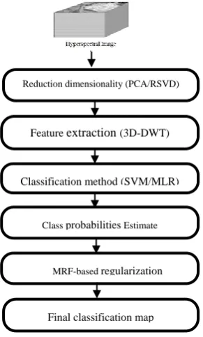
THE PROPOSED SYSTEM
[image:4.595.104.250.443.685.2]The Proposed system block-diagram is as shown in Figure 3, based on the works by [25, 1].
Fig. 3: The Proposed system Diagram
According to this work, the MAP-MRF framework based on Bayesian approach [25, 1], a pixel belonging to a class
c
is very likely to have neighboring pixels belonging to the same class. The Hammersly-Clifford theorem [42] is used to compute the MAP estimate ofy
as:
S
i i j
j i i
i
y p y x y y
yˆ argmin log ( / ) ( ) , (17)
where the term
p
(
y
i/
x
i)
is the spectral energy functionfrom the observed data, which needs to be estimated by probabilistic methods. Parameter μ is tunable and controls the degree of smoothness, and δ(y) is the unit impulse function, where δ(0) = 1 and δ(y) = 0 for
y
0
.
In this paper, The work has extended by applying a different classifiers methods based on PCA-3DDWT and RSVD-DDWT which discussed in sections 2,3 for reduction dimensionality and Feature Extraction , - on the final pixel-level segmentation results. The Proposed System Block-Diagram can be summarized basically, in the following steps:
1.Reduction dimensionality by PCA/RSVD 2.Feature Extraction by 3D-DWT
3.Classification (Learning): The posterior probability
pixelwise classification p(y/x,D)
i
i for a given pixel i x
and
the class label
i
y
can be obtained as:y
i
c
,
if: ), / ( ) , /
(y c x D p y c x D
p i i i t i ctc (18)
Various probabilistic classification techniques have been used to process hyperspectral data [43]. In this paper, SVM and MLRsub classifiers are used for probability estimations.
4. Segmentation: which infers an image of class labels from a posterior distribution built on the learned selected classifier and on a multilevel logistic (MLL) prior on the image of labels.
The final output of the algorithm is based on a maximum posteriori (MAP) segmentation process which is computed via an efficient min-cut-based integer optimization technique. The proposed Bayesian method exhibits good discriminatory capability when dealing with ill-posed problems, i.e., limited training samples versus high dimensionality of the input data and proposed approach provides class posterior probabilities which are crucial to the complete posterior probabilities, so that the final MAP segmentation can benefit from the inclusion of both the spectral and the spatial information available in the original hyperspectral data. The proposed method applies PCA/RSVD instead of considering the full spectral information as an input to the classifier models. Thus, it‘s able to circumvent some limitations in the techniques due to the high dimensionality of the input data and the presence of highly mixed pixels. The different components that have been used in the development of the proposed method are described. First, probabilistic pixelwise classification methods are used to know the posterior probability distributions from the spectral information. Second, the contextual information is used, by means of an MRF regularization scheme to refine the classification results as in figure 3. Estimating class conditional probability distributions is an intrinsic issue for the subsequent MRF-based classification.
5.
EXPERIMENTAL RESULTS
The suggested approach (Methods) has been tested on two real Hyperspectral images (HSI) benchmark datasets1: The Indian Pines dataset and Pavia University dataset, in variety of experimental settings. All the experiments were implemented
1: http://www.ehu.eus/ccwintco/index.php?title=Hyperspectral_Remote-sensing-Scenes
Feature extraction (3D-DWT)
Classification method (SVM/MLR)
Class probabilities Estimate
MRF-based regularization
Final classification map
in Matlab R2016b on a PC with Intel(R) core™ i5-3210M CPU @2.50GHz and 8GB RAM.
AVIRIS Indian pines Data
[image:5.595.325.518.201.350.2]This data set was gathered by Airborne Visible/Infrared Imaging Spectrometer (AVIRIS) sensor over the Indian Pines test site in Northwestern Indiana in June 1992. The original dataset contains 220 spectral reflectance bands in the wavelength range 0.4–2.5 µm, of which 20 bands covering the region of water absorption are removed and thus only 200 bands are reserved in this work. This scene has a spectral resolution of 10 nm and a spatial resolution of 20 m by pixel, and the spatial dimension is 145×145. The ground truth contains 16 land cover classes. The number of pixels in each class ranges unbalanced from 20 to 2468, which poses a big challenge for the classification task and is demonstrated in Table 6.1. A sample band of this image and the related ground truth data are shown in Figure 4.
(a) (b)
Fig. 4: Indian Pines image and ground truth categorization information. (a) The original HSI. (b) The
ground truth categorization map.
Table 1: Groundtruth classes for the Indian Pines scene and their respective samples number
No. Class Samples
1 Alfalfa 46 2 Corn-notill 1428 3 Corn-mintill 830 4 Corn 237 5 Grass-pasture 483 6 Grass-trees 730 7 Grass-pasture-mowed 28 8 Hay-windrowed 478 9 Oats 20 10 Soybean-notill 972 11 Soybean-mintill 2455 12 Soybean-clean 593 13 Wheat 205 14 Woods 1265 15
Buildings-Grass-Trees-Drives
386 16 Stone-Steel-Towers 93 Total 10,249
ROSIS Pavia University Data
This dataset was acquired by the Reflective Optics System Imaging Spectrometer (ROSIS) over the urban area of the University of Pavia, northern Italy, on July 8, 2002. The original dataset consists of 115 spectral bands ranging from 0.43 to 0.86 µm, of which 12 noisy bands are removed and only 103 bands are retained in our experiments. This scene has a spatial resolution of 1.3 m per pixel, and the spatial dimension is 610×340. There are 9 land cover classes in this scene and the number of each class is displayed in Table 2. Besides, a sample band of this image and the corresponding ground truth map are depicted in Figure 5.
Classification Accuracy
Assessment matrices are used to evaluate the result of the output classification/segmentation map based on the confusion matrix. This matrix provides a possibility for evaluating the exactitude of a given classification map with respect to the reference map. Several specific and global estimators are extracted from the confusion matrix. The term
i
C represents the class i and the term Cij refers to the number
of pixels which are wrongly assigned to the class j, which are referenced as class i.
C
N represents the number of classes in
the referenced map.
(a) (b)
Fig5:Pavia University image and related ground truth categorization information. (a) The original
HSI. (b) The ground truth categorization map
Table 2: Groundtruth classes for the Pavia University scene and their respective samples number
No. Class Samples
1 Asphalt 6631
2 Meadows 18649
3 Gravel 2099
4 Trees 3064
5 Painted metal sheets 1345
6 Bare Soil 5029
7 Bitumen 1330
8 Self-Blocking Bricks 3682
9 Shadows 947
Total 42,776
Overall Accuracy (OA)
The OA is the percentage of correctly classified pixels, which can be estimated as follows:
. 100
,
X C C OA
C C
N j
i ij
N
i ii
(19)
Class Accuracy (CA)
The CA is regarded as the percentage of correctly classified pixels for each class. It is calculated by dividing the number of correct pixels in one class by the total number of pixels as derived from reference data as follows:
. 100 X C C CA
C
N j ij
ii i
[image:5.595.56.274.253.375.2] [image:5.595.62.273.406.611.2] [image:5.595.63.272.408.612.2] Average Accuracy (AA)
The AA is the mean of class accuracies for all the classes, which can be estimated as follows:
. 100 X CA C AA
C N
j i
ii
(21)
Kappa Coefficient (k)
The k is a statistical measurement of agreement between the final classification map and the reference map:
e e o
p p p k
1
(22)
Where: p OA,
o
,
1
2
NC
i i i
e C C
N
p
,C
N j
ij
i C
C
C
N j
ji
i C
C
.
For all criteria, a larger value indicates a better classification performance. Firstly, to evaluate the validity of proposed method with number of labeled samples, 15% samples are chosen randomly for each class from the reference data as training samples, and the remaining samples in each class are used to test. This experiment is repeated 20 times. Secondly, the feature reduction techniques (i.e., PCA and RSVD) that were applied to the Hyperion dataset and the features extraction technique was applied by 3DDWT. The spatial-spectral classification methods were applied (i.e., SVM-MRF and MLRsub-MRF). For SVM-based methods, the RBF kernel parameter γ and the penalty parameter C are tuned through 5-fold cross validation (γ = 2−8, 2−7,...,28, C = 2−8,2−7,...,28). For MLRsub classifier, the smoothness parameter µ and the threshold parameter τ are set as in [38]. For PCA-3DDWT and RSVD-3DDWT, the number of principal components for PCA/RSVD is set as 20 in all experiments.
5.1
Experiments for the AVIRIS Dataset
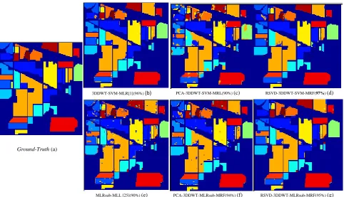
Classification maps for all the competing methods on Indian dataset are shown in Figure 6, and the accuracies (i.e. the classification accuracy of each class, OA, AA and kappa coefficient κ) are reported and compared in Table 3. From Figure 6 and Table 3, one main result can be highlighted: RSVD-3DDWT-SVM-MRF performs the best in terms of all the three criteria (OA, AA and κ) and attains a large improvement in this scenario, with PCA-3DDWT-SVM-MRL and MLRsub-MLL trailing slightly behind (90% OA). As shown in Table 3, although only 15% labeled samples for each class (10,249samples in total) are selected in the Indian Pines data. The OA of RSVD-3DDWT-SVM-MRF can reach 97%, about 7% higher than that of MLRsub-MLL (90%). Moreover, it can be also easily observed that the classification map of RSVD-3DDWT-SVM-MRF is more closely related to the ground truth map and it achieved the best performance in terms of all the three criteria (OA, AA and kappa coefficient κ).
5.2
Experiments for the Pavia University
Dataset
In this experiment, all parameters involved in the competing methods are tuned in the same way as the previous Indian Pines experiment. Classification maps obtained by all competing methods on Pavia University dataset are displayed in Figure 7, and the accuracies (i.e. the classification accuracy of each class, OA, AA and kappa coefficient κ) are summarized in Table 4. It can be also easily observed that the classification map of RSVD-3DDWT-SVM-MRF is leaded to the highest classification OA (96%), even though the number of training sample for each class is only 15% from training sample, which indicates the superiority of the RSVD-3DDWT-SVM-MRF in the scenario of small number of
[image:6.595.55.279.107.221.2]labeled training samples. As to PCA-3DDWT-SVM-MRL, PCA-3DDWT-MLRsub-MRF and RSVD-3DDWT-MLRsub-MRF, they achieve comparable classification OA (85%, 94% and 95%, respectively). Also, it is worthy to be emphasized that RSVD-3DDWT performs better than PCA-3DDWT, which can be found by comparing the OA of RSVD-3DDWT-SVM-MRF (96%) and PCA-3DDWT-SVM-MRL (85%) in Table 4. Meanwhile, it can be visually seen from Figure 7 that RSVD-3DDWT-SVM-MRF obtains much smoother classification map than 3DDWT-SVM-MLR. Besides, it should be noted that the RSVD-3DDWT-SVM-MRF achieves 4% higher OA than MLRsub-MLL, and 11% higher OA than PCA-3DDWT-SVM-MRL The RSVD-3DDWT-SVM-MRF is 1% higher than RSVD-3DDWT-MLRsub-MRF, which indicates that the classification accuracy can be obviously improved by adopting MRF to model the property of label smoothness. In addition, RSVD-3DDWT-SVM-MRF and RSVD-3DDWT-MLRsub-MRF achieve good and comparable performance because of the application of RSVD/PCA with 3DDWT feature. Consequently, the superiority of RSVD-3DDWT-SVM-MRF approach can be explained by use of RSVD-3DDWT and MRF, simultaneously.
6.
Conclusions and future work
In this paper, a novel technique is proposed for HSI classification. The key idea is to simultaneously utilize spatial-filtering method and spatial smoothness prior of labels. In this way, the spatial correlation under HSIs can be fully discovered. The RSVD/PCA with 3-dimensional discrete wavelet transform (3D-DWT) is utilized to extract the spectral-spatial features and the probabilistic SVM is used to character the spectral information of the new version of HSI cube reformulated by 3D-DWT. The local correlation of neighboring pixels is encoded by Markov random field (MRF). By computing the MAP classification with an optimized αExpansion graph-cut-based algorithm, the proposed classification method is efficient. Experimental results on two real benchmark hyperspectral data sets show that the proposed method outperforms the state of-the-art methods investigated in this paper. In our future research, there are still some tasks for future: firstly, the proposed algorithm has to be applied on other real HSI datasets images to achieve more reliable analysis of classification errors. Secondly, we want to use other classifiers to achieve more accurate characterization of the spectral-spatial Hyperspectral image classification according to classification map results. Finally, we will analyze in depth the complexity of our method to improve processing time.
7.
ACKNOWLEDGMENTS
Table 3: Classification Accuracies (%) of all competing methods on the Indian Pines image test set
class
3DDWT-SVM-MRF[1]
PCA
MLRsubMLL [25]
RSVD
3DDWT-MLRsub-MRF
3DDWT-SVM-MRF
3DDWT-MLRsub-MRF
3DDWT-SVM-MRF
1 100 96 100 67 100 100
2 97 93 90 92 97 97
3 96 92 78 84 93 96
4 94 98 95 86 92 95
5 93 88 89 93 93 98
6 97 99 99 96 98 97
7 95 69 100 95 95 95
8 100 99 100 99 100 100
9 80 90 100 88 76 91
10 89 91 89 86 89 99
11 96 94 71 92 97 96
12 93 96 90 81 92 97
13 97 100 100 95 97 95
14 95 97 84 93 95 98
15 99 65 99 86 99 99
16 86 97 93 86 86 89
OA 96 94 90 90 95 97
AA 94 92 92 88 93 96
K 95 93 89 89 94 96
Table 4: Classification accuracy (%) of all competing methods on the Pavia University dataset test set.
class
3DDWT-SVM-MRF[1]
PCA
MLRsubMLL[25]
RSVD
3DDWT-MLRsub-MRF
3DDWT-SVM-MRF
3DDWT-MLRsub-MRF
3DDWT-SVM-MRF
1 98 92 78 98 95 99
2 96 97 81 92 93 97
3 89 87 79 88 86 91
4 97 96 93 94 97 96
5 99 99 96 99 98 96
6 92 97 84 93 94 99
7 88 96 94 95 95 98
8 91 84 81 83 83 86
9 99 98 99 96 98 99
OA 95 94 85 92 95 96
AA 94 93 86 90 92 94
K 94 93 80 91 93 95
Ground-Truth (a)
3DDWT-SVM-MLR[1](95%)
PCA-3DDWT-SVM-MRL(85%)
RSVD-3DDWT-SVM-MRF(96%) 3DDWT-SVM-MLR[1](96%) (b) PCA-3DDWT-SVM-MRL(90%) (c) RSVD-3DDWT-SVM-MRF(97%) (d)
MLRsub-MLL [25 ](92%)
PCA-3DDWT- MLRsub-MRF(94%)
RSVD-3DDWT- MLRsub-MRF(95%) MLRsub-MLL [25](90%) (e) PCA-3DDWT-MLRsub-MRF(94%) (f) RSVD-3DDWT-MLRsub-MRF(95%) (g)
[image:7.595.53.544.392.769.2]8.
REFERENCES
[1] Cao, X. , Xu, L., Meng, D., Zhao, Q., and Xu, Z., , 2016 ―Integration of 3-dimensional discrete wavelet transform and Markov random field for hyperspectral image classification‖, Neurocomputing journal, [http://dx.doi.org/10.1016/j.neucom.2016.11.034]
[2] El-Rahman, S. A., Aliady, W. A., and Alrashed, N. I. 2015, ‖Supervised Classification Approaches to Analyze Hyperspectral Dataset‖, I. J. Image, Graphics and Signal Processing, pages 42–48.
[3] Jensen, R., 2005, ―Introductory digital image processing‖, Pearson Prentice Hall.
[4] Plaza, A., Martinez, P., Perez, R. and Plaza, J., 2004, ‖A new approach to mixed pixel classification of hyperspectral imagery based on extended morphological profiles‖, Pattern Recognition, 37, 1097–1116.
[5] Benediktsson, J.A., Palmason, J.A. and Sveinsson, J.R, 2005, ―Classification of hyperspectral data from urban areas based on extended morphological profiles‖, IEEE Trans. Geo-science Remote Sens. 43, 480–491.
[6] Ghamisi, P., Dalla Mura, M., Benediktsson, J.A, 2015. ‖A survey on spectral–spatial classification techniques based on attribute profiles‖, IEEE Trans. Geo-science Remote Sens. 53, 2335–2353.
[7] Tuia, D., Volpi, M., Dalla Mura, M., Rakotomamonjy, A. and Flamary, R., 2014. ―Automatic feature learning for spatio-spectral image classification with sparse SVM‖, IEEE Trans. Geo-science. Remote Sens. 52, 6062–6074.
[8] Dalla Mura, M., Villa, A., Benediktsson, J.A., Chanussot, J. and Bruzzone, L, 2011. ‖ Classification of hyperspectral images by using extended morphological attribute profile sand independent component analysis‖, IEEE Geo-science Remote Sens. Letter 8, 542–546.
[9] Jia, S., Zhang, X. and Li, Q., 2015. ―Spectral–spatial hyperspectral image classification using regularized low-rank representation and sparse representation-based graph cuts‖, IEEE J. Sel. Top. Appl. Earth Obs. Remote Sens. 8, 2473–2484.
[10] Zhang, X., Xu, C., Li, M. and Sun, X, 2015. ―Sparse and Low-rank coupling image segmentation model via non-convex regularization‖, Int. J. Pattern Recognition Artificial Intelligence.
Ground-Truth (a)
3DDWT-SVM-MLR[1](95%)
PCA-3DDWT-SVM-MRL(85%)
RSVD-3DDWT- SVM-MRF(96%)
3DDWT-SVM-MLR[1](95%) (b) PCA-3DDWT-SVM-MRL(85%) (c) RSVD-3DDWT-SVM-MRF(96%) (d)
MLRsub-MLL [25 ](92%)
PCA-3DDWT- MLRsub-MRF(94%)
RSVD-3DDWT- MLRsub-MRF(95%)
[image:8.595.72.538.73.492.2][11] Zhang, B., Li, S., Jia, X., Gao, L. and Peng, M., 2011. ―Adaptive Markov Random field approach for classification of hyperspectral imagery‖. IEEE Geoscience Remote Sens. Letter, 8, 973–977.
[12] Tarabalka, Y. and Rana, A., 2014. ― Graph-cut-based model for spectral-spatial classification of hyperspectral images‖, In Proceedings of the 2014 IEEE Geoscience and Remote Sensing Symposium, Quebec, QC, Canada, 13–18, pp. 3418–3421.
[13] Pajares, G., Lópezmartínez, C., Sánchezlladó, F.J. and Molina, I., 2012. ―Improving Wishart classification of polarimetric SAR data using the Hopfield neural network optimization approach‖. Remote Sens. 4, 3571–3595.
[14] Guijarro, M., Pajares, G. and Herrera, P.J., 2009. ―Image-based airborne sensors: A combined approach for spectral signatures classification through deterministic simulated annealing‖, Sensors,9, 7132–7149.
[15] Sánchez-Lladó, F.J., Pajares, G. and López-Martínez, C., 2011. ―Improving the Wishart synthetic aperture radar image classifications through deterministic simulated annealing‖, ISPRS J. Photogramm. Remote Sens. 66, 845–857.
[16] Zhong, Y., Ma, A. and Zhang, L., 2014. ―An adaptive Memetic fuzzy clustering algorithm with spatial information for remote sensing imagery‖. IEEE J. Sel. Top. Appl. Earth Obs. Remote Sens., 7, 1235–1248.
[17] Qian, Y., Ye, M. and Zhou, J., 2013. ―Hyperspectral image classification based on structured sparse logistic regression and three-dimensional wavelet texture features‖, IEEE Trans. Geo-science Remote Sens., 51, 2276–2291.
[18] Shen, L. and Jia, S., 2011. ―Three-dimensional Gabor wavelets for pixel-based hyperspectral imagery classification‖ IEEE Trans. Geo-science Remote Sens., 49, 5039–5046.
[19] Tang, Y., Lu, Y. and Yuan, H., 2015. ―Hyperspectral image classification based on three-dimensional scattering wavelet transform‖, IEEE Trans. Geoscience Remote Sens., 53, 2467–2480.
[20] Zhang, L., Zhang, L., Tao, D. and Huang, X., 2013 ―Tensor discriminative locality alignment for hyperspectral image spectral–spatial feature extraction‖, IEEE Trans. Geoscience Remote Sens., 53, 242–256.
[21] Zhang, L., Zhang, Q., Zhang, L., Tao, D., Huang, X. and Du, B., 2015. ―Ensemble manifold regularized sparse low-rank approximation for multiview feature embedding‖, Pattern Recognition, 48, 3102–3112.
[22] Melgani, F., and Bruzzone, L., 2004. ―Classification of hyperspectral remote sensing images with support vector machines,‖ IEEE Trans. Geosci. Remote Sens., vol. 42, no. 8, pp. 1778–1790.
[23] Chen, Y., Nasrabadi, N. M. and Tran, T. D., 2011. ―Simultaneous joint sparsity model for target detection in hyperspectral imagery,‖ IEEE Geo-science. Remote Sens. Letter, vol. 8, no. 4, pp. 676–680.
[24] Chen, Y., Nasrabadi, N. M. and Tran, T. D., 2011. ―Hyperspectral image classification using dictionary
based sparse representation‖, IEEE Trans. Geo-science. Remote Sens., vol. 49, no. 10, pp. 3973–3985.
[25] Li, J., BioucasDias, J. M. and Plaza, A., 2012. ―Spectral-spatial hyperspectral image segmentation using subspace multinomial logistic regression and Markov random field,‖ IEEE Trans. Geoscience Remote Sens., vol. 50, no. 3, pp. 809–823.
[26] Camps-Valls, G., Gomez-Chova, L., Muñoz-Marí, J., Vila-Francés, J. and CalpeMaravilla, J., 2006. ―Composite kernels for hyperspectral image classification‖, IEEE Geoscience and Remote Sensing Letters 3 (1) , 93–97.
[27] Gu, Y., Wang, Q., Wang, H., You, D. and Zhang, Y., 2015. ―Multiple kernel learning via low-rank nonnegative matrix factorization for classification of hyperspectral imagery‖, IEEE Journal of Selected Topics in Applied Earth Observations and Remote Sensing 8 (6), 2739–2751.
[28] Böhning, D., 1992. ―Multinomial logistic regression algorithm‖, Annals of the Institute of Statistical Mathematics 44 (1) 197–200.
[29] Qian, Y., Ye, M. and Zhou, J., 2013. “Hyperspectral image classification based on structured sparse logistic regression and three-dimensional wavelet texture features‖, IEEE Transactions on Geoscience and Remote Sensing 51 (4), 2276–2291.
[30] Zhao, W. and Du, S., 2016. ―Spectral–spatial feature extraction for hyperspectral image classification: A dimension reduction and deep learning approach‖, IEEE Trans. Geoscience Remote Sens., 54, 4544–4554.
[31] Yue, J., Zhao, W., Mao, S. and Liu, H., 2015. ―Spectral-spatial classification of hyperspectral images using deep convolutional neural networks‖. Remote Sens. Letter, 6, 468–477.
[32] Makantasis, K., Karantzalos, K., Doulamis,A., Doulamis,N., 2015. ―Deep supervised learning for hyperspectral data classification through convolutional neural networks‖. In Proceedings of the IEEE International Geoscience and Remote Sensing Symposium, Milan, Italy, 26–31, pp. 4959–4962.
[33] Liang, H. and Li, Q., 2016. ―Hyperspectral imagery classification using sparse representations of con- volutional neural network features”. Remote Sens., 8.
[34] Martinsson P.G. and Voronin S., 2015. ‖A Randomized blocked Algorthim for Efficiently Computing Rank-Revealing Factorizations of Matrices.‖, arXiv preprint, pp. 1-26.
[35] Erichson N. B., Voronin, S., Brunton S. L., Kutz J. N., 2017. ‖ Randomized Matrix Decompositions using R‖, Journal of Statistical Software, arXiv:1608.02148v3, 3.
[36] Chun-Lin, L., 2010. ―A tutorial of the wavelet transform‖, NTUEE, Taiwan.
[38] Camps-Valls, G. and Bruzzone, L., 2005. ‖Kernel-based methods for hyperspectral image classification‖, IEEE Transactions on Geoscience and Remote Sensing, 43(6):1351–1362.
[39] Wu, T.-F., Lin, C.-J. and Weng, R. C., 2004. ―Probability estimates for multi-class classification by pairwise coupling‖. Journal of Machine Learning Research, 5:975–1005.
[40] Lin, C.-J., Lin, H.-T. and Weng, R. C., 2003. ―A note on Platt‘s probabilistic outputs for support vector machines‖, Department of Computer Science, National Taiwan University, Taipei, Taiwan.
[41] Chang, C. and Lin, C., 2009. ―LIBSVM: A library for support vector machines‖.
[42] Clifford, P., 1990. ― Markov random fields in statistics‖, In Geoffrey Grimmett and Dominic Welsh, editors, Disorder in Physical Systems: A Volume in Honour of John M. Hammersley, pages 19–32. Oxford University Press, Oxford,
![Figure 1 illustrates the computation steps involved to compute the randomized SVD [35]](https://thumb-us.123doks.com/thumbv2/123dok_us/9297047.427460/2.595.314.543.105.440/figure-illustrates-computation-steps-involved-compute-randomized-svd.webp)