Semi supervised Stochastic Multi Domain Learning using Variational Inference

Proceedings of the 57th Annual Meeting of the Association for Computational Linguistics, pages 1923–1934 1923

Semi-supervised Stochastic Multi-Domain Learning using Variational

Inference

Yitong Li Timothy Baldwin

School of Computing and Information Systems The University of Melbourne, Australia

[email protected] {tbaldwin,tcohn}@unimelb.edu.au

Trevor Cohn

Abstract

Supervised models of NLP rely on large col-lections of text which closely resemble the in-tended testing setting. Unfortunately matching text is often not available in sufficient quantity, and moreover, within any domain of text, data is often highly heterogenous. In this paper we propose a method to distill the important do-main signal as part of a multi-dodo-main learning system, using a latent variable model in which parts of a neural model are stochastically gated based on the inferred domain. We compare the use of discrete versus continuous latent vari-ables, operating in a domain-supervised or a domain semi-supervised setting, where the do-main is known only for a subset of training in-puts. We show that our model leads to substan-tial performance improvements over compet-itive benchmark domain adaptation methods, including methods using adversarial learning.

1 Introduction

Text corpora are often collated from several dif-ferent sources, such as news, literature, micro-blogs, and web crawls, raising the problem of learning NLP systems from heterogenous data, and how well such models transfer to testing set-tings. Learning from these corpora requires mod-els which can generalise to different domains, a problem known as transfer learning or domain adaptation (Blitzer et al.,2007;Daum´e III,2007; Joshi et al.,2012;Kim et al.,2016). In most state-of-the-art frameworks, the model has full knowl-edge of the domain of instances in the training data, and the domain is treated as a discrete in-dicator variable. However, in reality, data is often messy, with domain labels not always available, or providing limited information about the style and genre of text. For example, web-crawled cor-pora are comprised of all manner of text, such as news, marketing, blogs, novels, and recipes,

how-ever the type of each document is typically not ex-plicitly specified. Moreover, even corpora that are labelled with a specific domain might themselves be instances of a much more specific area, e.g., “news” articles will cover politics, sports, travel, opinion, etc. Modelling these types of data accu-rately requires knowledge of the specific domain of each instance, as well as the domain of each test instance, which is particularly problematic for test data from previously unseen domains.

A simple strategy for domain learning is to jointly learn over all the data with a single model, where the model is not conditioned on domain, and directly maximisesp(y|x), wherexis the text input, and y the output (e.g. classification label). Improvements reported in multi-domain learning (Daum´e III, 2007; Kim et al., 2016) have often focused on learning twin representations (shared

andprivaterepresentations) for each instance. The private representation is modelled by introduc-ing a domain-specific channel conditional on the domain, and the shared one is learned through domain-general channels. To learn more robust domain-general and domain-specific channels, ad-versarial supervision can be applied in the form of either domain-conditional or domain-generative methods (Liu et al.,2016;Li et al.,2018a).

out when the domain is unobserved. We pro-pose a sequence of models of increasing complex-ity in the modelling of the treatment of z, rang-ing from a discrete mixture model, to a contin-uous vector-valued latent variable (analogous to a topic model; Blei et al. (2003)), modelled us-ing Beta or Dirichlet distributions. We show how these models can be trained efficiently, using ei-ther direct gradient-based methods or variational inference (Kingma et al.,2014), for the respective model types. The variational method can be ap-plied to domain and/or label semi-supervised set-tings, where not all components of the training data are fully observed.

We evaluate our approach using sentiment anal-ysis over multi-domain product review data and 7 language identification benchmarks from dif-ferent domains, showing that in out-of-domain evaluation, our methods substantially improve over benchmark methods, including adversarially-trained domain adaptation (Li et al.,2018a). We show that including additional domain unlabelled data gives a substantial boost to performance, re-sulting in transfer models that often outperform domain-trained models, to the best of our knowl-edge, setting a new state of the art for the dataset.

2 Stochastic Domain Adaptation

In this section, we describe our proposed ap-proaches to Stochastic Domain Adaptation (SDA), which use latent variables to represent an implicit ‘domain’. This is formulated as a joint model of output classification label,yand latent domainz, which are both conditional onx,

p(y, z|x) =pφ(z|x)pθ(y|x,z).

The two components are the prior, pφ(z|x), and classifier likelihood,pθ(y|x,z), which are

param-eterised byφandθ, respectively. We propose sev-eral different choices of prior, based on the nature of z, that is, whether it is: (i) a discrete value (“DSDA”, see Section 2.2); or (ii) a continuous vector, in which case we experiment with different distributions to model p(z|x) (“CSDA”, see Sec-tion2.3).

2.1 Stochastic Channel Gating

For all of our models the likelihood, pθ(y|x,z),

is formulated as a multi-channel neural model, where z is used as a gate to select which chan-nels should be used in representing the input. The

model comprises k channels, with each channel computing an independent hidden representation,

hi= CNNi(x;θ)|ki=1

using a convolutional neural network.1 The value ofzis then used to select the channel, by comput-ing h = Pk_i=1zkhi, where we assume z ∈ Rk is a continuous vector. For the discrete setting, we represent integerzby its 1-hot encodingz, in which caseh = hz. The final step of the

likeli-hood passesh through a MLP with a single hid-den layer, followed by a softmax, which is used to predict class labely.

2.2 Discrete Domain Identifiers

We now turn to the central part of our method, the prior component. The simplest approach, DSDA

(see Figure1a), uses a discrete latent variable, i.e., z ∈ [1, k] is an integer-valued random variable, and consequently the model can be considered as a form of mixture model. This prior predicts z given input x, which is modelled using a neural network with a softmax output. Givenz, the pro-cess of generatingyis as described above in Sec-tion2.1. The discrete model can be trained for the maximum likelihood estimate using the objective,

logp(y|x) = log k X

z=1

pφ(z|x)pθ(y|x, z), (1)

which can be computed tractably,2 and scales lin-early ink.

DSDAcan be applied with supervised or semi-supervised domains, by maximising the likelihood p(z = d|x) when the ground truth domain dis observed. We refer to this setting as “DSDA+sup.” or “DSDA+semisup”, respectively, noting that in

this setting we assume the number of channels,k, is equal to the known inventory of domains,D.

2.3 Continuous Domain Identifiers

For the DSDAmodel to work well requires suffi-ciently largek, such that all the different types of data can be clearly separated into individual mix-ture components. When there is not a clear delin-eation between domains, the inferred domain pos-terior is likely to be uncertain, and the approach

1_{Our approach is general, and could be easily combined}

with other methods besides CNNs.

x CNNk(θk)

CNN1(θ1)

· · ·

hk h1

· · · J

h y

CNN(φ) _p

z

(a)DSDA

x CNNk(θk)

CNN1(θ1)

· · ·

hk h1

· · · J

h y

CNN(σ)

CNN(φ) _p

q

∼ b z y, d

DKL

(b)CSDA

Figure 1: Model architectures for latent variable models,DSDA andCSDA, which differ in the treatment of the latent variable, which is discrete (d∈[1, k]), or a continuous vector (ˆz∈Rk). The lower green model components

showkindependent convolutional network components, and the blue and yellow component the prior,p, and the variational approximation,q, respectfully. The latent variable is used to gate thekhidden representations (shown

asJ

), which are then used in a linear function to predict a classification label,y. During trainingCSDAdraws samples (∼) fromq, while during inference, samples are drawn fromp.

reduces to an ensemble technique. Thus, we in-troduce the second modelling approach as Con-tinuous domain identifiers (CSDA), inspired by the way in which LDA models the documents as mix-tures of several topics (Blei et al.,2003).

A more statistically efficient method would be to use binary functions as domain specifiers, i.e., z∈ {0,1}k_{, effectively allowing for exponentially}

many domain combinations (2k). Each element of the domain zi acts as a gate, or equivalently,

at-tention, governing whether hidden statehi is

in-corporated into the predictive model. In this way, individual components of the model can specialise to a very specific topic such as politics or sport, and yet domains are still able to combine both to produce specialised representations, such as the politics of sport. The use of a latent bit-vector renders inference intractable, due to the marginal-isation over exponentially many states. For this reason, we instead make a continuous relaxation, such thatz∈ Rkwith each scalarzi being drawn

from a probability distribution parameterised as a function of the inputx. These functions can learn to relate aspects ofxwith certain domain indexes, e.g., the use of specific words likebaseballand in-ningsrelate to a domain corresponding to “sport”, thereby allowing the text domains to be learned automatically.

Several possible distributions can be used to model z ∈ _Rk_{. Here we consider the following}

distributions:

Beta which bounds all elements to the range

[0,1], such thatzlies in a hyper-cube;

Dirichlet which also bounds all elements, as for Beta, howeverzare also constrained to lie in the probability simplex.

In both cases,3 each dimension ofz is controlled by different distribution parameters, themselves formulated as different non-linear functions ofx. We expect the Dirichlet model to perform the best, based on their widespread use in topic models, and their desirable property of generating a normalised vector, resembling common attention mechanisms (Bahdanau et al.,2015).

Depending on the choice of distribution, the prior is modelled as

p(z|x) = Beta αααB, βββB (2a)

or p(z|x) = Dirichlet α0αααD

, (2b)

where the prior parameters are parameterised as neural networks of the input. For the Beta prior,

αααB = elu(fα,B(x)) + 1 (3a)

β β

βB = elu(fβ,B(x)) + 1, (3b)

where elu(·) + 1 is an element-wise activation function which returns a positive value (Clevert et al.,2016), andfω(·)is a nonlinear function with

parametersω—here we use a CNN. The Dirichlet prior uses a different parameterisation,

α0 = exp(fD,0(x)) (4a)

αααD = sigmoid(fD(x)), (4b)

3_{We also compared Gamma distributions, but they}

where α0 is a positive-valued overall concentra-tion parameter, used to scale all components in (2b), thus capturing overall sparsity, while αααD models the affinity to each channel.

2.4 Variational Inference

Using continuous latent variables, as described in Section 2.3, gives rise to intractable inference; for this reason we develop a variational infer-ence method based on the variational auto-encoder (Kingma and Welling, 2014). Fitting the model involves maximising the evidence lower bound (ELBO),

logpφ,θ(y|x) = log Z

z

pφ(z|x)pθ(y|z,x)

≥_E

qσ[logpθ(y|z,x)] (5)

−λDKL qσ(z|x, y, d)||pφ(z|x)

,

where qσ is the variational distribution,

param-eterised by σ, chosen to match the family of the prior (Beta or Dirichlet) and λ is a hyper-parameter controlling the weight of the KL term. The ELBO in (5) is maximised with respect to σ, φandθ, using stochastic gradient ascent, where the expectation term is approximated using a sin-gle sample, ˆz ∼ qσ, which is used to compute

the likelihood directly. Although it is not nor-mally possible to backpropagate gradients through a sample, which is required to learn the varia-tional parametersσ, this problem is usually side-stepped using a reparameterisation trick (Kingma and Welling, 2014). However this method only works for a limited range of distributions, most notably the Gaussian distribution, and for this rea-son we use the implicit reparameterisation gradi-ent method (Figurnov et al.,2018), which allows for inference with a variety of continuous distribu-tions, including Beta and Dirichlet. We give more details of the implicit reparameterisation method in AppendixA.2.

The variational distribution q, is defined in an analagous way to the prior,p, see (2–4b), i.e., us-ing a neural network parameterisation for the dis-tribution parameters. The key difference is that q conditions not only on xbut also on the target label y and domain d. This is done by embed-ding bothyandd, which are concatenated with a CNN encoding ofx, and then transformed into the distribution parameters. Semi-supervised learning with respect to the domain can easily be facili-tated by setting d to the domain identifier when

it is observed, otherwise using a sentinel value d = UNK, for domain-unsupervised instances. The same trick is used fory, to allow for vanilla semi-supervised learning (with respect to target la-bel). The use ofyanddallows the inference net-work to learn to encode these two key variables into z, to encourage the latent variable, and thus model channels, to be informative of both the tar-get label and the domain. This, in concert with the KL term in (5), ensures that the prior,p, must also learn to discriminate for domain and label, based solely on the input text,x.

For inference at test time, we assume that only xis available as input, and accordingly the infer-ence network cannot be used. Instead we generate a sample from the priorˆz∼p(z|x), which is then used to compute the maximum likelihood label,

ˆ

y = arg max_yp(y|x,ˆz). We also experimented with Monte Carlo methods for test inference, in order to reduce sampling variance, using: (a) prior mean ¯z = µ; (b) Monte Carlo averaging y¯ =

1

m P

ip(y|x,zˆi) using m = 100 samples from

the prior; and (c) importance sampling (Glynn and Iglehart,1989) to estimate p(y|x) based on sam-pling from the inference network,q.4 None of the Monte Carlo methods showed a significant differ-ence in predictive performance versus the single sample technique, although they did show a very tiny reduction in variance over 10 runs. This is de-spite their being orders of magnitude slower, and therefore we use a single sample for test inference hereafter.

3 Experiments

3.1 Multi-domain Sentiment Analysis

To evaluate the proposed models, we first ex-periment with a multi-domain sentiment analy-sis dataset, focusing on out-of-domain evaluation where the test domain is unknown.

We derive our dataset from Multi-Domain Sen-timent Dataset v2.0 (Blitzer et al., 2007).5 The task is to predict a binary sentiment label, i.e., pos-itive vs. negative. The unprocessed dataset has more than 20 domains. For our purposes, we filter out domains with fewer than 1k labelled instances

4_{Importance sampling estimates p(y|x) =}

Eq[p(y,z|x)/q(z|x, y, d)] for each setting of y using m= 100samples fromq, and then finds the maximisingy. This is tractable in our settings asy is a discrete variable, e.g., a binary sentiment, or multiclass language label.

5_From

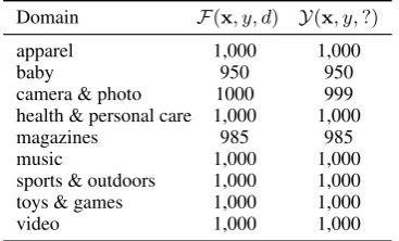
Domain F(x, y, d) Y(x, y,?)

apparel 1,000 1,000

baby 950 950

camera & photo 1000 999 health & personal care 1,000 1,000

magazines 985 985

music 1,000 1,000

sports & outdoors 1,000 1,000 toys & games 1,000 1,000

video 1,000 1,000

Table 1: Numbers of instances (reviews) for each train-ing domain in our dataset, under the two categoriesF (domain and label known) andY(label known; domain unknown), in which “?” represents the “UNK” token, meaning the given attribute is unobserved.

or fewer than 2k unlabelled instances, resulting in 13 domains in total.

To simulate the semi-supervised domain situa-tion, we remove the domain attributions for one half of the labelled data, denoting them as domain-unlabelled data Y(x, y,?). The other half are sentiment- and domain-labelled data F(x, y, d). We present a breakdown of the dataset in Table1.6 For evaluation, we hold out four domains— namely books (“B”), dvds (“D”), electronics (“E”), and kitchen & housewares (“K”)—for com-parability with previous work (Blitzer et al.,2007). Each domain has 1k test instances, and we split this data into dev and test with ratio 4:6. The

devdataset is used for hyper-parameter tuning and early stopping,7and we report accuracy results on

test.

3.1.1 Baselines and Comparisons

For comparison, we use 3 baselines. The first is a single channel CNN (“S-CNN”), which jointly

over all data instances in a single model, with-out domain-specific parameters. The second base-line is a multi channel CNN (“M-CNN”), which

expands the capacity of the S-CNN model (606k parameters) to match CSDA and DSDA (roughly 7.5m-8.3m parameters). Our third baseline is a multi-domain learning approach using adversarial learning for domain generation (“GEN”), the best-performing model ofLi et al.(2018a) and state-of-the-art for unsupervised multi-domain adaptation over a comparable dataset.8 We report results for

6

The dataset, along with the source code, can be found at https://github.com/lrank/Code_ VariationalInference-Multidomain

7

This confers light supervision in the target domain. However we would expect similar results were we to use dis-joint held out domains for development wrt testing.

8

The dataset used inLi et al.(2018a) differs slightly in that it is also based off Multi-Domain Sentiment Dataset v2.0,

their best performingGEN+d+gmodel.

3.1.2 Training Strategy

For the hyper-parameter setups, we provide the details in Appendix A.1. In terms of training, we simulate two scenarios using two experimental configurations, as discussed above: (a) domain su-pervision; and (2) domain semi-supervision. For domain supervised training, onlyFis used, which covers only 9 of the domains, and the test do-main data is entirely unseen. For dodo-main semi-supervised training, we use combinations of F

and Y, noting that both sub-corpora do not in-clude data from the target domains, and none of which is explicitly labelled with sentiment,y, and domain, d. These simulate the setting where we have heterogenous data which includes a lot of rel-evant data, however its metadata is inconsistent, and thus cannot be easily modelled.

For λin (5), according to the derivation of the ELBO it should be the case thatλ = 1, however other settings are often justified in practice (Alemi et al., 2018). Accordingly, we tried both anneal-ing and fixed schedules, but found no consistent differences in end performance. We performed a grid search for the fixed value, λ = 10a, a ∈ {−3,−2,−1,0,1}, and selectedλ= 10−1, based on development performance. We provide further analysis in the form of a sensitivity plot in Sec-tion3.2. The latent domain sizekforDSDAis set to the true number of training domainsk = D = 9. Note that, even forDSDA, we could usek6=D, which we explore in theF+Ysupervision setting in Section3.1.3. For CSDA we present the main

results withk= 13, set to match the total number of domains in training and testing.

3.1.3 Results

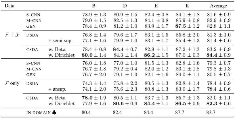
Table2reports the performance of different mod-els under two training configurations: (1) with

F+Y(domain semi-supervised learning); and (2) withFonly (domain supervised learning). In each case, we report the standard deviation based on 10 runs with different random seeds.

Overall, domain B and D are more difficult than E and K, consistent with previous work. Comparing the two configurations, we see that when we use domain semi-supervised training (with the addition of Y), all models perform

Data B D E K Average

F+Y

S-CNN 78.9±1.3 80.9±1.5 82.4±0.8 84.1±1.8 81.6±0.9 M-CNN 79.0±1.5 82.5±1.3 84.1±0.8 85.9±0.8 82.9±0.9 GEN 78.4±0.9 81.2±1.0 83.9±1.7 87.5±1.2 82.8±1.1

DSDA 76.8±1.4 79.6±1.7 83.1±1.5 85.8±2.0 81.3±1.0

+ semi-sup. 77.1±1.6 79.9±1.0 83.1±1.7 85.4±1.3 81.4±0.6

CSDA w.Beta 78.4±0.8 84.4±0.7 82.9±1.1 87.2±1.3 83.2±0.9

w.Dirichlet 80.0±1.4 84.3±1.4 86.2±1.5 87.0±0.3 84.4±0.9

Fonly

S-CNN 76.0±1.8 77.0±1.0 81.5±1.3 82.8±1.6 79.3±0.7 M-CNN 76.7±1.8 79.2±0.4 82.0±1.2 83.1±1.8 79.8±1.3 GEN 76.7±2.0 79.1±1.3 82.1±1.6 84.0±1.1 80.5±0.7

DSDA 74.3±1.4 75.8±2.2 80.5±1.3 82.8±1.4 78.4±0.9

+ unsup. 74.1±2.0 75.6±2.3 80.8±1.3 83.0±1.7 78.4±0.6

CSDA w.Beta 78.0±1.9 80.5±1.1 83.7±1.3 85.7±1.3 82.0±1.1

w.Dirichlet 77.9±1.6 80.6±0.9 84.4±1.1 86.5±0.9 82.3±0.6

IN DOMAIN♣ 80.4 82.4 84.4 87.7 83.7

Table 2: Accuracy [%] and standard deviation of different models under two data configurations: (1) using both F andY (domain semi-supervised learning); and (2) usingF only (domain supervised learning). In each case, we evaluate over the four held-out test domains (B, D, E and K), and also report the accuracy. Best results are indicated inboldin each configuration. Key:♣fromBlitzer et al.(2007).

ter, demonstrating the utility of domain semi-supervised learning when annotated data is lim-ited.

Comparing our discrete and continuous ap-proaches (DSDA and DSDA, resp.), we see that CSDAconsistently performs the best, outperform-ing the baselines by a substantial margin. In con-trast DSDAis disappointing, underperforming the

baselines, and moreover, shows no change in per-formance between domain supervision versus the semi-supervised or unsupervised settings. Among theCSDAbased methods, all the distributions per-form well, but the Dirichlet distribution perper-forms the best overall, which we attribute to better mod-elling of the sparsity of domains, thus reducing the influence of uncertain and mixed domains. The best results are for domain semi-supervised learn-ing (F+Y), which brings an increase in accuracy of about 2% over domain supervised learning (F) consistently across the different types of model.

3.2 Analysis and Discussion

To better understand what the model learns, we fo-cus on theCSDAmodel, using the Dirichlet distri-bution.

First, we consider the model capacity, in terms of the latent domain size, k. Figure 2shows the impact of varyingk. Note that the true number of domains isD = 13, comprising 9 training and 4 test domains. Settingk to roughly this value ap-pears to be justified, in that the mean accuracy

2 4 8 16 32 64

76 78 80 82 84

k

Acc

Figure 2: Performance with standard error (|||) as latent domain sizek is increased inlog 2 space with DSDA ( ) and with threeCSDAmethods usingBeta( ) and Dirichlet( ) averaged accuracy, overF+Y.

increases with k, and plateaus around k = 16. Interestingly, when k ≥ 32, the performance of

CSDA with Beta drops, while performance for

Dirichletremains high—indeedDirichletis con-sistently superior even at the extreme value of k = 2, although it does show improvement as k increases. Also observe thatDSDArequires a large latent state inventory, supporting our argument for the efficiency of continuous cf. discrete latent vari-ables.

Next, we consider the impact of using differ-ent combinations ofF andY. Table3shows the performance of difference configurations. Overall,

Domain B D E K apparel baby

camera & photo health & personal care magazines

music

sports & outdoors toys & games video Sentiment negative positive

Figure 3: t-SNE of hidden representations inCSDAover all 13 domains, comprising 4 held-out testing domains (B, D, E and K), and the remaindering 9 domains are used only for training. Each point is a document, and the symbol indicates its gold sentiment label, using a filled circle for negative instances and cross for positive.

CSDA B D E K Average

F 77.9 80.6 84.4 86.5 82.3 F+Y 80.0 84.3 86.2 87.0 84.4 Y 77.6 81.5 83.7 85.2 82.0

Table 3: Accuracy [%] ofCSDA w. Dirichlet trained with different configurations ofFandY.

Y on its own is only a little worse than only F, showing that target labelsyare more important for learning than the domaind. TheY configuration fully domain unsupervised training still results in decent performance, boding well for application to very messy and heterogenous datasets with no domain metadata.

Finally, we consider what is being learned by the model, in terms of how it learns to use the k dimensional latent variables for different types of data. We visualise the learned representations, showing points for each domain plotted in a 2d t-SNE plot (Maaten and Hinton,2008) in Figure3. Notice that each domain is split into two clus-ters, representing positive (×××) and negative (•) in-stances within that domain. Among the test do-mains,B(books) andD(dvds) are clustered close together but are still clearly separated, which is en-couraging given the close relation between these two media. The other two, E (electronics) and

K(kitchen & housewares) are mixed together and intermingled with other domains. Overall across all domains, theAPPARELcluster is quite distinct,

0.001 0.01 0.1 1 10

20 40 60 80 100

λ

Acc

y d

Figure 4: Diagostic classifier accuracy [%] over zto predict the sentiment labelyand domain labeld, with respect to differentλ, shown on a log scale. Dashed horizontal lines show chance accuracy for both outputs.

while VIDEO and MUSIC are highly associated with D, and part of the cluster for MAGAZINES

is close to B; all of these make sense intuitively, given similarities between the respective products. E is related to CAMERA and GAMES, while Kis most closely connected toHEALTHandSPORTS.

Data EUROGOV TCL WIKIPEDIA EMEA EUROPARL TBE TSC Average

Y

S-CNN 98.8 92.3 85.9 98.5 92.3 79.3 91.7 91.3

M-CNN 98.9 93.6 86.2 99.2 96.0 88.3 91.7 93.4

DSDA 98.3 91.9 86.3 97.8 95.2 86.0 79.0 90.6

CSDA w.Beta 98.7 93.0 89.0 99.3 96.8 93.1 95.2 95.0

w.Dirichlet 98.9 93.0 89.0 99.2 96.7 93.2 94.5 94.9

F

DSDA 98.0 91.8 85.7 97.7 95.3 85.4 78.1 90.3

CSDA w.Beta 99.3 93.7 89.1 99.2 96.9 93.6 93.9 95.1

w.Dirichlet 99.0 93.7 89.3 99.3 96.9 93.3 96.1 95.4

GEN 99.9 93.1 88.7 92.5 97.1 91.2 96.1 94.1

LANGID.PY 98.7 90.4 91.3 93.4 97.4 94.1 92.7 94.0

Table 4: Accuracy [%] over 7 LangID benchmarks, as well as the averaged score, for different models under two data configurations: (1) using domain unsupervised learning (Y); and (2) using domain supervised learning (F). The best results are indicated inboldin each configuration. Note that the training data forGENandLANGID.PYis slightly different from that used in the original papers.

record samples of z from the inference network. We then partition the training set, using 70% to learn linear logistic regression classifiers to predict yandd, and use the remaining 30% for evaluation. Figure4shows the prediction accuracy, based on averaging over three runs, each with different z samples. Clearly very smallλ ≤ 10−2, leads to almost perfect sentiment label accuracy which is evidence of overfitting by using the latent variable to encode the response variable. For λ ≥ 10−1

the sentiment accuracy is still above chance, as ex-pected, but is more stable. For the domain labeld, the predictive accuracy is also above chance, albeit to a lesser extent, and shows a similar downward trend. At the setting λ = 0.1, used in the ear-lier experiments, this shows that the latent variable encodes captures substantial sentiment, and some domain knowledge, as observed in Figure3.

In terms of the time required for training, a sin-gle epoch of training took about 25min for the

CSDA method, using the default settings, and a similar time for DSDAand M-CNN. The runtime increases sub-linearly with increasing latent size k.

3.3 Language Identification

To further demonstrate our approaches, we then evaluate our models with the second task, lan-guage identification (LangID: Jauhiainen et al. (2018)).

For data processing, we use 5 training sets from 5 different domains with 97 language, following the setup ofLui and Baldwin(2011). We evaluate accuracy over 7 holdout benchmarks: EUROGOV, TCL, WIKIPEDIA fromBaldwin and Lui(2010), EMEA (Tiedemann,2009), EUROPARL (Koehn,

2005), TBE (Tromp and Pechenizkiy,2011) and TSC (Carter et al., 2013). Differently from sen-timent tasks, here, we evaluate our methods us-ing the full dataset, but with two configurations: (1) domain unsupervised, where all instance have only labels but no domain (denotedY); and (2) do-main supervised learning, where all instances have labels and domain (F).

3.3.1 Results

Table4shows the performance of different mod-els over 7 holdout benchmarks and the averaged scores. We also report the results ofGEN, the best model fromLi et al.(2018a), and one state-of-the-art off-the-shelf LangID tool: LANGID.PY (Lui and Baldwin,2012). Note that, both S-CNN and M-CNN are domain unsupervised methods. In terms of results, overall, both of our CSDA els consistently outperform all other baseline mod-els. Comparing the differentCSDAvariants,Beta

vs. Dirichlet, both perform closely across the LangID tasks. Furthermore, CSDA out-performs

the state-of-the-art in terms of average scores. In-terestingly the two training configurations show that domain knowledge F provides a small per-formance boost for CSDA, but not does help for

DSDA. Above all, the LangID results confirm the effectiveness of our proposed approaches.

4 Related Work

knowledge of the target domain (Blitzer et al., 2007; Glorot et al., 2011). Adversarial learn-ing methods have been proposed for learnlearn-ing ro-bust domain-independent representations, which can capture domain knowledge through semi-supervised learning (Ganin et al.,2016).

Multi-domain adaptation uses training data from more than one training domain. Approaches include feature augmentation methods (Daum´e III, 2007), and analagous neural models (Joshi et al., 2012; Kim et al., 2016), as well as attention-based and hierarchical methods (Li et al.,2018b). These works assume the ‘oracle’ source domain is known when transferring, however we do not require an oracle in this paper. Adversarial train-ing methods have been employed to learn robust domain-generalised representations (Liu et al., 2016). Li et al. (2018a) considered the case of the model having no access to the target domain, and using adversarial learning to generate domain-generation representations by cross-comparison between source domains.

The other important component of this work is Variational Inference (“VI”), a method from ma-chine learning that approximates probability den-sities through optimisation (Blei et al.,2017; Ku-cukelbir et al., 2017). The idea of a variational auto-encoder has been applied to language gener-ation (Bowman et al.,2016;Kim et al.,2018;Miao et al.,2017;Zhou and Neubig,2017;Zhang et al., 2016) and machine translation (Shah and Barber, 2018;Eikema and Aziz,2018), but not in the con-text of semi-supervised domain adaptation.

5 Conclusion

In this paper, we have proposed two models—

DSDA and CSDA—for multi-domain learning, which use a graphical model with a latent variable to represent the domain. We propose models with a discrete latent variable, and a continuous vector-valued latent variable, which we model with Beta or Dirichlet priors. For training, we adopt a vari-ational inference technique based on the varia-tional autoencoder. In empirical evaluation over a multi-domain sentiment dataset and seven lan-guage identification benchmarks, our models out-perform strong baselines, across varying data con-ditions, including a setting where no target domain data is provided. Our proposed models have broad utility across NLP applications on heterogenous corpora.

Acknowledgements

This work was supported by an Amazon Research Award. We thank the anonymous reviewers for their helpful feedback and suggestions.

References

Alexander Alemi, Ben Poole, Ian Fischer, Joshua Dil-lon, Rif A Saurous, and Kevin Murphy. 2018. Fix-ing a broken elbo. InInternational Conference on Machine Learning, pages 159–168.

Dzmitry Bahdanau, Kyunghyun Cho, and Yoshua Ben-gio. 2015. Neural machine translation by jointly learning to align and translate. In Proceedings of the International Conference on Learning Represen-tations.

Timothy Baldwin and Marco Lui. 2010. Language

identification: The long and the short of the mat-ter. InProceedings of Human Language Technolo-gies: Conference of the North American Chapter of the Association of Computational Linguistics, pages 229–237.

David M Blei, Alp Kucukelbir, and Jon D McAuliffe. 2017. Variational inference: A review for statisti-cians. Journal of the American Statistical Associa-tion, 112(518):859–877.

David M Blei, Andrew Y Ng, and Michael I Jordan. 2003. Latent Dirichlet allocation. Journal of Ma-chine Learning Research, 3(Jan):993–1022.

John Blitzer, Mark Dredze, and Fernando Pereira.

2007. Biographies, Bollywood, boom-boxes and

blenders: Domain adaptation for sentiment classi-fication. In Proceedings of the 45th Annual Meet-ing of the Association of Computational LMeet-inguistics, pages 440–447.

Samuel R. Bowman, Luke Vilnis, Oriol Vinyals, An-drew Dai, Rafal Jozefowicz, and Samy Bengio.

2016. Generating sentences from a continuous

space. InProceedings of The 20th SIGNLL Confer-ence on Computational Natural Language Learning, pages 10–21.

Simon Carter, Wouter Weerkamp, and Manos

Tsagkias. 2013. Microblog language identification: Overcoming the limitations of short, unedited

and idiomatic text. Language Resources and

Evaluation, 47(1):195–215.

Djork-Arn´e Clevert, Thomas Unterthiner, and Sepp Hochreiter. 2016. Fast and accurate deep network learning by exponential linear units (ELUs). In Pro-ceedings of the International Conference on Learn-ing Representations.

Bryan Eikema and Wilker Aziz. 2018. Auto-encoding

variational neural machine translation. arXiv

preprint arXiv:1807.10564.

Mikhail Figurnov, Shakir Mohamed, and Andriy Mnih. 2018. Implicit reparameterization gradients. In Ad-vances in Neural Information Processing Systems 31, pages 439–450.

Yaroslav Ganin, Evgeniya Ustinova, Hana Ajakan, Pascal Germain, Hugo Larochelle, Franc¸ois Lavi-olette, Mario Marchand, and Victor Lempitsky. 2016. Domain-adversarial training of neural

net-works. Journal of Machine Learning Research,

17:59:1–59:35.

Xavier Glorot, Antoine Bordes, and Yoshua Bengio. 2011. Domain adaptation for large-scale sentiment classification: A deep learning approach. In Pro-ceedings of the 28th International Conference on Machine Learning, pages 513–520.

Peter W Glynn and Donald L Iglehart. 1989. Impor-tance sampling for stochastic simulations. Manage-ment Science, 35(11):1367–1392.

Tommi Jauhiainen, Marco Lui, Marcos Zampieri, Tim-othy Baldwin, and Krister Lind´en. 2018. Automatic language identification in texts: A survey. CoRR, abs/1804.08186.

Mahesh Joshi, Mark Dredze, William W. Cohen, and Carolyn Penstein Ros´e. 2012. Multi-domain

learn-ing: When do domains matter? InProceedings of

the 2012 Joint Conference on Empirical Methods in Natural Language Processing and Computational Natural Language Learning, pages 1302–1312.

Yoon Kim. 2014. Convolutional neural networks for sentence classification. InProceedings of the 2014 Conference on Empirical Methods in Natural Lan-guage Processing, pages 1746–1751.

Yoon Kim, Sam Wiseman, Andrew Miller, David

Son-tag, and Alexander Rush. 2018. Semi-amortized

variational autoencoders. InProceedings of the 35th International Conference on Machine Learning,

vol-ume 80 of Proceedings of Machine Learning

Re-search, pages 2678–2687.

Young-Bum Kim, Karl Stratos, and Ruhi Sarikaya. 2016. Frustratingly easy neural domain adaptation. In Proceedings of COLING 2016, the 26th Inter-national Conference on Computational Linguistics: Technical Papers, pages 387–396.

Diederik P. Kingma and Jimmy Ba. 2015. Adam: A method for stochastic optimization. InProceedings of the International Conference on Learning Repre-sentations.

Diederik P. Kingma, Shakir Mohamed, Danilo Jimenez Rezende, and Max Welling. 2014. Semi-supervised learning with deep generative models. InAdvances in Neural Information Processing Systems 27: An-nual Conference on Neural Information Processing Systems 2014, pages 3581–3589.

Diederik P Kingma and Max Welling. 2014. Auto-encoding variational Bayes. InProceedings of the International Conference on Learning Representa-tions.

Philipp Koehn. 2005. Europarl: A parallel corpus for statistical machine translation. InMT Summit 2005, pages 79–86.

Alp Kucukelbir, Dustin Tran, Rajesh Ranganath, An-drew Gelman, and David M Blei. 2017. Automatic differentiation variational inference. Journal of Ma-chine Learning Research, 18(1):430–474.

Yitong Li, Timothy Baldwin, and Trevor Cohn. 2018a. What’s in a domain? learning domain-robust text representations using adversarial training. In Pro-ceedings of the 2018 Conference of the North Amer-ican Chapter of the Association for Computational Linguistics: Human Language Technologies, Vol-ume 2 (Short Papers), pages 474–479.

Zheng Li, Ying Wei, Yu Zhang, and Qiang Yang. 2018b. Hierarchical attention transfer network for cross-domain sentiment classification. In Proceed-ings of the Thirty-Second AAAI Conference on Arti-ficial Intelligence.

Pengfei Liu, Xipeng Qiu, and Xuanjing Huang. 2016. Deep multi-task learning with shared memory for text classification. InProceedings of the 2016 Con-ference on Empirical Methods in Natural Language Processing, pages 118–127.

Marco Lui and Timothy Baldwin. 2011. Cross-domain feature selection for language identification. InFifth International Joint Conference on Natural Lan-guage Processing, pages 553–561.

Marco Lui and Timothy Baldwin. 2012. langid.py:

An off-the-shelf language identification tool. In Proceedings of ACL 2012 System Demonstrations, pages 25–30.

Laurens van der Maaten and Geoffrey Hinton. 2008. Visualizing data using t-SNE. Journal of Machine Learning Research, 9(Nov):2579–2605.

Yishu Miao, Edward Grefenstette, and Phil Blunsom. 2017. Discovering discrete latent topics with neu-ral variational inference. InProceedings of the 34th International Conference on Machine Learning-Volume 70, pages 2410–2419.

Harshil Shah and David Barber. 2018. Generative neu-ral machine translation. InAdvances in Neural In-formation Processing Systems, pages 1346–1355.

J¨org Tiedemann. 2009. News from OPUS – a collec-tion of multilingual parallel corpora with tools and interfaces. InRecent Advances in Natural Language Processing, volume 5, pages 237–248.

InProceedings of the 20th Machine Learning Con-ference of Belgium and The Netherlands, pages 27– 34.

Biao Zhang, Deyi Xiong, Jinsong Su, Hong Duan, and Min Zhang. 2016. Variational neural machine trans-lation. In Proceedings of the 2016 Conference on Empirical Methods in Natural Language Process-ing, pages 521–530.

Chunting Zhou and Graham Neubig. 2017.

Multi-space variational encoder-decoders for

semi-supervised labeled sequence transduction. In

A Appendices

A.1 Base Model Architecture

For the sentiment task, all the hidden representa-tions are learned by convolutional neural networks (CNN), followingKim(2014). All documents are lower-cased and truncated to maximum 256 to-kens, and then each word is mapped into a 300 di-mensional vector representation using randomly-initialised word embeddings. In eachCNN chan-nel, filter windows are set to {3,4,5}, with 128 filters for each. Then,ReLUandpoolingare ap-plied after the filtering, generating384-d (128∗3) hidden representations. Dropout is applied to the hiddenh, at a rate of 0.5. For simplicity, we use the same CNN architecture to encode the func-tionsfused in the priorqand in the inference net-works p, in each case with different parameters. Specifically, in priorq, the embedding sizes of do-main and label are set to 16 and 4, respectively.ααα andβββshare the sameCNNbut with different out-put projections. After gating usingz, the final hid-den goes through a one-hidhid-denMLPwith hidden size 300. We use the Adam optimiser (Kingma and Ba, 2015) throughout, with the learning rate set to10−4and a batch size of 32, optimising the loss functions (1) or (5), forDSDAandCSDA,

re-spectively.

For the language identification task, all docu-ments are tokenized as a byte sequence, truncated or padded to a length of 1k bytes. We use the same

CNNarchitecture and hyper-parameter configura-tions as for the sentiment task.

A.2 Implicit Reparameterisation Gradient

In this section, we outline the implicit reparam-eterisation gradient method of Figurnov et al. (2018). First, we review some background on vari-ational inference. We start by defining a differen-tiable and invertible standardization function as

Sσ(z) =∼q(), (6a)

which describes a mapping between points drawn from a specific distribution function and a stan-dard distribution, q. For example, for a Gaus-sian distribution z ∼ N(µ, ψ), we can define Sµ,ψ(z) = (z−µ)/ψ ∼ N(0,1)to map to the

standard Normal. We aim to compute the gradient of the expectation of a objective functionf(z),

∇_{σ E}

qσ(z)

[f(z)] = _E q()

[∇_σf(S−1())], (6b)

where in ELBO (5) in our case,f(z) =pθ(y|z,x)

is the likelihood function.

The implicit reparameterisation gradient tech-nique is a way of computing the reparameterisa-tion without the need for inversion of the stan-dardization function. This works by applying

∇_σS−1() =∇_σz,

∇_{σ E}

qσ(z)

[f(z)] = _E qσ(z)

[∇_zf(z)∇_σz]. (6c)

However, we still need to calculate∇σz. The key

insight here is that we can compute ∇_σz by im-plicit differentiation. We apply the total gradient

∇TD

σ over (6a),

∇TD_σ Sσ(z) =∇TD_σ . (6d)

From the definition of a standardization function, the noiseis independent ofσ, and we apply the multi-variable chain rule over left side of (6d),

∂Sσ(z)

∂z ∇σz+

∂Sσ(z)

∂σ =0. (6e)

Therefore, the key of the implicit gradient calcula-tion in this process can be summarised as

∇σz=−(∇zSσ(z))−1∇σSσ(z). (6f)