Forecasting bubbles with mixed causal noncausal autoregressive models

Munich Personal RePEc Archive

Forecasting bubbles with mixed

causal-noncausal autoregressive models

Voisin, Elisa and Hecq, Alain

Maastricht University

13 March 2019

Online at

https://mpra.ub.uni-muenchen.de/96350/

Forecasting bubbles with mixed

causal-noncausal autoregressive models

Alain Hecq and Elisa Voisin

Maastricht University

August, 2019

Abstract

This paper investigates one-step ahead density forecasts of mixed causal-noncausal models. It analyses and compares two data-driven approaches. The paper focuses on explosive episodes and therefore on predicting turning points of bubbles. Guidance in using these approximation methods are presented with the suggestion of using both of the approaches as they jointly carry more information. The analysis is illustrated with an application on Nickel prices.

Keywords: noncausal models, forecasting, predictive densities, bubbles, simulations-based forecasts.

JEL.C22, C53

1_{Corresponding author : Elisa Voisin, Maastricht University, Department of} Quanti-tative Economics, School of Business and Economics, P.O.box 616, 6200 MD, Maastricht, The Netherlands. Email: e.voisin@maastrichtuniversity.nl.

1

Introduction

Locally explosive episodes have long been observed in financial and economic time series. Such patterns, often observed in stock prices, can be triggered by anticipation or speculation. Given this forward-looking aspect, expecta-tion models have been prevalent for modelling them. As shown for instance by Gouri´eroux, Jasiak, and Monfort (2016), equilibrium rational expecta-tion models admit a multiplicity of soluexpecta-tions, and some of them feature such speculative bubble patterns.2 _{Models employed to capture them range from}

simplistic approaches, such as single bubble models with constant probabil-ity of crash, to rather complex models depending on numerous parameters. Although those models may a posteriori fit the data well, they are either not informative enough or render predictions uncertain due to their dependence on extensive parameters estimation.

This paper analyses and compares two data-driven approaches to perform density forecasts of mixed causal-noncausal autoregressive (hereafterMAR) models. MAR models incorporate both lags and leads of the dependent variable with potentially heavy-tailed errors. The most commonly used distributions for such models in the literature are the Cauchy and Stu-dent’s t-distributions. While being parsimonious, MAR models generate non-linear dynamics such as locally explosive episodes in a strictly station-ary setting (Fries and Zako¨ıan, 2019). So far, the focus has mainly been put on identification and estimation. Hecq, Lieb, and Telg (2016), Hencic and Gouri´eroux (2015) and Lanne, Luoto, and Saikkonen (2012) show that model selection criteria favour the inclusion of noncausal components ex-plaining respectively the observed bubbles in the demand of solar panels in Belgium, in Bitcoin prices and in inflation series. Few papers look at the forecasting aspects. Gouri´eroux and Zako¨ıan (2017) derive theoretical point and density forecasts of purely noncausal MAR(0,1) processes with Cauchy-distributed errors, for which the causal conditional distribution ad-mits closed-form expressions. With some other distributions however, like Student’s t, conditional moments and distribution may not admit closed-form expressions. Lanne, Luoto, and Saikkonen (2012) and Gouri´eroux and Jasiak (2016) developed data-driven estimators to approximate them based

on simulations or on past realised values respectively, applicable to any dis-tribution. Nonetheless, the literature regarding the ability of MAR models to predict both explosive and stable episodes remains scarce (see also Lanne, Nyberg, and Saarinen, 2012 and Gouri´eroux, Hencic, and Jasiak, 2018). The aim of this paper is to analyse and compare in details the two numerical methods mentioned for forecastingMAR(r,1) models, with unconstrainedr

number of lags, a unique lead and a positive lead coefficient. Furthermore, the focus is put on positive bubbles since they are prevalent in financial and economic time series. This paper investigates the possibility to predict, one-step ahead, probabilities of turning points of locally explosive episodes. We find that the sample-based method is characterised by a learning mechanism and that the simulations-based approach is a good approximation of theo-retical results. Our results show that combining results obtained from the two methods can help disentangling the proportion of probabilities induced by the underlying distribution and by past behaviours. This information could for instance be used for investment decisions, where the strategy is to be built based on the investor’s risk aversion and beliefs regarding the series.

The paper is constructed as follows. Section 2 introduces mixed causal-noncausal autoregressive models. Section 3 discusses how they have been used for prediction so far when the conditional moments and densities admit closed-form expressions. In Section 4 are presented the simulations-based forecasting approach proposed by Lanne, Luoto, and Saikkonen (2012), fol-lowed by the sample-based method proposed by Gouri´eroux and Jasiak (2016). The performance of both approaches is compared, when available, to theoretical results. The analysis is based on variousMAR(0,1) processes with Cauchy or Student’s t-distributed errors. In Section 5 both approxi-mation methods are illustrated with an application to a detrended Nickel prices series. Section 6 concludes.

2

Mixed causal-noncausal autoregressive models

Consider the univariateMAR(r,s) process defined as follows,

Φ(L)Ψ(L−1

)yt=εt,

where L and L−₁

are respectively the lag and forward operators; Φ and Ψ are two invertible polynomials of degree r and s respectively. That is, Φ(L) = (1−φ1L· · · −φrLr) and Ψ(L−1) = (1−ψ1L−1· · · −ψsL−s) with

a non-Gaussian distribution. This assumption, not empirically restrictive since non-normality is widely observed in financial and economic time series, is necessary to achieve identification of the model. AnMAR(r,s) model can also be expressed as a causal AR model where yt depends on its own past

and present value ofut,

Φ(L)yt=ut, (1)

whereut is the purely noncausal component of the errors, depending on its

own future and on the present value of the error term

Ψ(L−₁

)ut=εt. (2)

Alternatively, we can also filter the process as Φ(L)vt=εtwith Ψ(L−1)yt=

vt to obtain the backward component of the errors, vt. The process yt

admits a stationary infinite two-sided MA representation and depends on past, present and future values of εt,

yt=

+∞

X

i=−∞ aiεt−i.

The case in which all coefficientsai for −∞< i≤0 (resp. 0≤i <∞) are

equal to 0, corresponds to a purely causal (resp. noncausal) model.

Despite their apparent simplicity and parsimony,MARmodels often provide a better fit to economic and financial data as they capture non-linear causal dynamics such as bubbles or asymmetric cycles. The shape of series gener-ated byMAR(r,s) processes depends on the presence of leads, lags and the magnitude of their coefficients. Figure 1 displays how the presence of a lag, a lead, or both, affects the shape of transitory shocks inMARseries. Purely causal (resp. noncausal) processes are only affected by a shock after (resp. before) the impact; this is shown in graph (a) (resp. (b)). Consequently,

MAR processes are affected both in anticipation and after the shock; the shape of the explosive episode (mostly forward or backward looking) depends on the magnitude of the lag and lead coefficients. When the coefficients are identical (c) the effects of the shock are symmetric around the impact while when the coefficient of the lead is higher (d), the explosive episode is more analogous to what we refer to as a bubble with an asymmetry around the peak.

Figure 1: Effects of a lag and a lead on transitory shocks forMARseries (a) purely causalφ= 0.8 and ψ= 0, (b) purely noncausal φ= 0 and ψ= 0.8, (c)φ= 0.8 and ψ= 0.8, (d)φ= 0.3 and ψ= 0.8

to distinguish between purely causal, noncausal or mixed processes as their autocovariance functions are identical. Fitting an autoregressive model by OLS allows however to estimate the sum of leads and lags,p.3 Subsequently, the respective numbers of lags (r) and leads (s), such that r+s= p, can be estimated by an approximate maximum likelihood (hereafter AML) ap-proach (Lanne and Saikkonen, 2011). The selected model is the one max-imising the AML with respect to r, s and all parameters Ω = (Φ,Ψ,Θ), where Φ = (φ1, . . . , φr), Ψ = (ψ1, . . . , ψs) and Θ is the errors distribution

parameters, such as the scale or location for instance. The AML estimator is defined as follows,

ˆ

Φ,Ψˆ,Θˆ=argmaxΦ,Ψ,Θ

T−_s

X

t=r+1

ln

gΦ(L)Ψ(L−₁

)yt; Θ

,

where g denotes the pdf of the error term, satisfying the regularity

con-3

ditions (Andrews, Davis, and Breidt, 2006). Lanne and Saikkonen (2011) show that the resulting (local) maximum likelihood estimator is consistent, asymptotically normal and that ( ˆΨ,Φ) and ˆˆ Θ are asymptotically indepen-dent, for Student’s t-distributed errors with finite moments. Since an ana-lytic solution of the maximisation problem at hand is not directly available, numerical gradient-based procedures can be employed. Hecq et al. (2016) indicate that estimatingMAR models is easier for more volatile series since the convergence of the estimator is empirically faster for distributions with fatter tails. They propose an alternative way to obtain the standard errors, a method implemented in the R package MARX (Hecq, Lieb, and Telg, 2017).

While with a unique lead and a positive coefficient ψ, explosive episodes increase at a fixed rateψ−₁

until a sudden crash, other specifications induce complex patterns not resembling the bubble pattern that this paper focuses on. This paper hence only considers MAR(r,1) processes with a positive lead coefficient.

3

Predictions using closed-form expressions

When it comes to forecastingMARprocesses, different approaches are avail-able. Conditional expectations can be used to predict the next points, while alternatively, forecasting densities aims at visually analysing the proba-bilities of potential future paths. The latter can be employed to evalu-ate the probabilities of a turning point in an explosive episode. However, the anticipative aspect of MAR models complicates their use for predic-tions. Results are not as straightforward as they could be with purely backward-looking ARMA models. While in some cases mean or density forecasts can be directly obtained from the assumed errors distribution, they sometimes need to be approximated. For this section, let us assume that the data generating process (hereafter dgp) is a stationary MAR(r,1) process Φ(L)(1−ψL−₁

)yt =εt, where ψ >0,εt is i.i.d. non-Gaussian and

ut= Φ(L)ytis the purely non-causal component of the process. Throughout

the coming sections, thedgp is be assumed correctly identified to disregard estimation uncertainty.

Given the true dgp, the information sets (y1, . . . , yT, y∗_T+1, . . . , y_T∗_+h) and

(v1, . . . , vr, εr+1, . . . , εT−₁, u_T, u ∗

T+1, . . . , u ∗

T+h), where vt = Φ(L)−1εt and

ut = (1−ψL−1)−1εt, are equivalent. This allows to predict future values

The asterisk indicates unrealised values of the random variables. Most prediction methods hence aim attention at purely noncausal processes – hereut, sufficient to predict the variable of interest.

3.1 Point predictions

Gouri´eroux and Zako¨ıan (2017) derive the first two conditional moments of

MAR(0,1) processes,4 here denoted as ut, and show that for Cauchy

pro-cesses, withψ >0, the expectation ofuT+1 conditioned on the information

set known at timeT,FT, is

E

uT+1|FT] =uT. (3)

This result is puzzling since the conditional expectation of a noncausal pro-cess has a unit root even though the propro-cess is stationary. Fries (2018) expanded those results to any admissible parametrisation of the tail and asymmetry parameters ofα-stable distributions and derives up to the fourth conditional moments. He also derives the limiting distribution of those four moments when the variable of interest diverges. He shows that during an explosive episode, the computation of those moments gets considerably sim-plified and are characteristic of a weighted Bernoulli distribution charging probability ψαh _{to the value ψ}−_h

uT and (1−ψαh) to value zero, for a tail

parameter 0< α <2. Those results indicate that along a bubble, the pro-cess can only either keep on increasing with fixed rate or drop to zero. For Cauchy-distributed errors (α = 1), the mean forecast during an explosive episode remains equal to Equation (3), yet for other α-stable distributions the conditional expectation may be drastically simplified. Hence, during an explosive episode, the point forecast of an MAR(0,1) process is a weighted average of the crash and further increase (e.g. a random walk for Cauchy-distributed processes). Density forecasts may therefore be more informative.

3.2 Density predictions

The joint conditional predictive density (as named by Gouri´eroux and Jasiak, 2016) or the causal transition distribution (as named by Gouri´eroux and Zako¨ıan, 2017) of the h future values, (u∗

T+1, . . . , u ∗

T+h), given the

in-formation known at time T can be evaluated only conditioning on the last observed value uT. This stems from the equivalence of information set of

the observed series and of its filtrations when the model is assumed correctly identified and the independence between the error components. While the interest is on predicting the future given present and past information, it is only possible, by the model definition, to derive the density of a point conditional on its future point. Bayes’ Theorem is first used to get rid of the conditioning on the present point and a second time to condition on the last point of the forecast. Then, the theorem is applied repeatedly on the first term until the density of all points is conditional on future ones. The conditionalpdf can thus be expressed as follows,

l(u∗

T+1, . . . , u ∗

T+h|uT)

=l(uT, u∗T+1, . . . , u ∗

T+h−1|u ∗

T+h)×

l(u∗

T+h)

l(uT)

=

l(uT|u∗T+1, . . . , u ∗

T+h)l(u

∗

T+1|u ∗

T+2, . . . , u ∗

T+h). . . l(u

∗

T+h−1|u ∗

T+h)

× l(u ∗

T+h)

l(uT)

,

whereldenotes densities associated with the noncausal processut. Equation

(2) states that εt = ut−ψut+1, hence, for all t, only ut+1 is necessary to

derive ut. Furthermore, given ut+1, the conditional density of ut (which is

not known) is equivalent to the density ofεt(which is known) evaluated at

the point ut−ψut+1.5 That is, for any assumed errors distribution g we

have,

l(u∗

T+1, . . . , u ∗

T+h|uT)

=nl(uT|u∗T+1)l(u ∗

T+1|u ∗

T+2). . . l(u ∗

T+h−1|u ∗

T+h)

o

×l(u ∗

T+h)

l(uT)

=g(uT −ψu

∗

T+1). . . g(u ∗

T+h−₁−ψu ∗

T+h)×

l(u∗

T+h)

l(uT)

.

(4)

Problems may however arise when the stationary distribution of ut is

unknown. We know that ut = ψut+1 +εt = P

∞

i=0ψiεt+i, but the pdf of

a linear combinations of errors may not admit closed-form expressions for some distributions.

5_Since

uτ =ψuτ+1+ετ and becauseuτ+1 andετ are independent for all 1≤τ ≤T,

we havefuτ|uτ+1(x) =fετ+ψuτ+1|uτ+1(x) =fετ|uτ+1(x−ψuτ+1) =fε(x−ψuτ+1). For

For instance, Gouri´eroux and Zako¨ıan (2013) present closed-form solutions for the predictive conditional density of purely noncausal MAR(0,1) pro-cesses with Cauchy-distributed errors. They show that the characteristic function of the infinite sum corresponds to that of a Cauchy with scale pa-rameter₍₁₋γ_ψ), whereγ is the scale of the distribution of the errorsεt. Hence,

in theMAR(r,1) case with Cauchy errors,ut∼Cauchy

0,₍₁₋γ_ψ). The pre-dictive density of the purely noncausal process (ut) can thus be computed

as such,

l(u∗

T+1, . . . , u ∗

T+h|uT)

= 1 (πγ)h

1

1 +(uT−ψu∗T+1) 2

γ2

. . . 1

1 +(u∗T+h−1−ψu∗T+h)

2

γ2

!

× γ

2_{+ (1−ψ)}2_u2

T

γ2_{+ (1−ψ)}2_(u∗

T+h)2

.

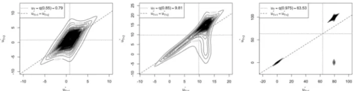
To illustrate how the predictive density evolves as the series departs from central values, Figure 2 shows one-step ahead forecasts for different levels corresponding to quantiles 0.55, 0.85 and 0.975 of a purely noncausal process with a lead coefficient of 0.8 and standard Cauchy-distributed errors. By using quantiles, explosive episodes can be compared between different distributions and parameters.6 While the predictive distribution is uni-modal for median-level values, it splits and becomes bi-modal when the series departs from such values. As the series diverges, the bi-modality of the conditional distribution becomes more evident, where the two modes correspond to a drop to 0 and a continuous increase with rate (1/0.8); each event has probability 0.2 and 0.8 respectively. Those results corroborate what Fries (2018) shows for diverging Cauchy-distributed

MAR(0,1) series. Note that results are analogous for any parameters, with corresponding probabilities of a crash equal to 1−ψ. Bi-modality in this paper will therefore designate the split of the conditional density and not the bi-modality sometimes observed in the estimation of the coefficients of

MAR models (Hecq et al., 2016 and Bec, Bohn Nielsen, and Sa¨ıdi, 2019)

ForMAR(r,1) processes, one-step ahead density forecasts consists in shifting the predictive density of the purely non-causal component by the causal part of the process, namelyφ1yT +...+φryT−r+1. For anh-step ahead forecast,

withh ≥1, the predictive density of y∗

T+h will depend on the joint density

6

Figure 2: Evolution of the 1-step ahead predictive density as the level of the series increases for a CauchyMAR(0,1) withψ= 0.8.

of (u∗

T+1, . . . , u ∗

T+h). One way of approaching this is to directly write the

predictive density in terms ofy∗

T+k, with 1≤k≤h, in the conditional joint

density of (u∗

T+1, . . . , u ∗

T+h). For an MAR(1,1) process with lag coefficient

φ for instance, the conditional predictive density of h future y’s could be obtained as follows,

l(y∗

T+1, . . . , y ∗

T+h|yT) =

1 (πγ)h

× 1

1 +(uT−ψ(yT∗+1−φyT)) 2

γ2

. . . 1

1 +(y∗T+h−1−φy∗T+h−2)−ψ(y∗T+h−φy∗T+h−1)) 2

γ2

× γ

2_{+ (1−ψ)}2_u2

T

γ2_{+ (1−ψ)}2_(y∗

T+h−φy

∗

T+h−₁)2 .

Figure 3 shows the evolution of two-step ahead forecasts of a purely noncausal process with lead coefficient 0.8 and Cauchy-distributed errors as the variable increases. For high levels of the series, the split of the distribution is evident; at each step the series can either keep on increasing or drop to zero, where the latter corresponds to an absorbing state. An interpretation of the regions of the graphs with respect to potential future shapes of the series was given by Gouri´eroux and Jasiak (2016).

Figure 3: Evolution of the 2-step ahead joint predictive density as the level of the series increases for anMAR(0,1) withψ= 0.8 and Cauchy-distributed errors

the densities by choosing a threshold, such as the last observed value or its half for instance. Nonetheless, as indicated by Fries (2018) for α-stable distributions, explosive episodes seem to be memoryless and as the series diverges, the probabilities of a crash tend to the constant 1−ψαh _{for given}

a given horizonh≥1. Even though ash→ ∞this probability tends to 1, it may not be very realistic when it comes to real life data. We might expect the probabilities of a crash in stock prices for instance to increase with the level of prices. Furthermore, the assumption of other fat-tail distributions (e.g. Student’s t) generally leads to the absence of closed-form expressions for the conditional moments and densities. The next Section presents two approaches to approximate the conditional densities in such circumstances; the first one is based on simulations (Lanne, Luoto, and Saikkonen, 2012) and the second one uses sample counterparts (Gouri´eroux and Jasiak, 2016).

4

Predictions using approximation methods

4.1 Predictions using simulations-based approximations

Lanne, Luoto, and Saikkonen (2012) base their methodology on the fact that the noncausal component of the errors, u, can be expressed as an infinite sum of future errors, which in theMAR(r,1) case is as follows,

ut= Ψ(L

−₁

)−₁ εt=

∞

X

i=0

ψiεt+i.

Since stationarity is assumed, and because in applications ψ rarely (and barely) exceeds 0.9, the sequence (ψi_{) converges rapidly to zero. Hence,}

point of the noncausal component of the errors can be approximated as the following finite sum,

u∗

T+h ≈ M−_h

X

i=0 ψiε∗

T+h+i, (5)

for any h≥1.

As explained before, any point forecast y∗

T+h of an MAR(r,1) process

depends on the sequence forecast (u∗

T+1, . . . , u ∗

T+h). Thus, forecasting

any future point y∗

T+h or the path (y

∗

T+1, . . . , y ∗

T+h), with h ≥ 1, requires

forecasting the sequence of M future errors (ε∗

T+1, . . . , ε ∗

T+M) which we

will denote as ε∗

+. Instead of deriving an M-dimensional conditional joint

density function (Lanne, Luoto, and Saikkonen (2012) use M = 50) , they propose a way to obtain conditional point and cumulative density forecasts. While the estimation approach they propose requires finite moments for the errors distribution, this restriction is not necessary for their forecasting method (Lanne and Saikkonen, 2011).

Using the companion form of anMAR(r,1) model, y∗

T+h can, by recursion,

be expressed as the sum of a known component and the h future values of

ut, where the latter, based on Equation (5), can be approximated as a linear

combination of M future errors

y∗

T+h =ι

′

ΦhyT + h−1

X

i=0 ι′

Φiιu∗

T+h−_i

≈ι′

ΦhyT + h−₁

X

i=0 ι′

Φiι

M−_h+i

X

j=0 ψjε∗

T+h−i+j,

(6)

where

yT =

     yT

yT−1

.. .

yT−r+1



   

, Φ=       

φ1 φ2 . . . φr

1 0 . . . 0 0 1 0 . . . 0 ..

. . .. ... ... ... 0 . . . 0 1 0

      

(r×r) and ι=      1 0 .. . 0     

(r×1).

Let g(ε∗

+|uT) be the conditional joint distribution of the M future errors,

which, using Bayes’ Theorem can be expressed as follows,

g(ε∗

+|uT) =

l(uT|ε∗+) l(uT)

Thus, for any functionq,

Ehq(ε∗ +) u_T i = Z

q(ε∗ +)g(ε

∗

+|uT)dε

∗ +

= 1

l(uT)

Z

q(ε∗

+)l(uT|ε

∗ +)g(ε

∗ +)dε

∗ +

= Eε ∗

+

h

q(ε∗

+)l(uT|ε∗+)

i

l(uT)

.

(7)

Similarly as before, l(uT|ε∗+) can be obtained from the errors distribution

g. Yet, since it is conditional on ε∗

+ instead of u ∗

T+1, we can only obtain

an approximation. Using this approximation and the Iterated Expectation theorem, the marginal distribution ofuT can be approximated as follows,

l(uT) =Eε∗

+

l(uT|ε

∗ +)

≈Eε∗

+

"

g uT − M

X

i=1 ψiε∗

T+i

!#

.

Overall, by plugging the aforementioned approximation in (7), we obtain

E

h

q(ε∗ +)

u_T

i

≈

Eε∗

+

"

q(ε∗ +)g

uT −PM_i=1ψiε∗_T+i

#

Eε∗+

"

guT −PMi=1ψiε ∗

T+i

# .

Letε∗₊(j) =ε∗_T(₊₁j), . . . , ε∗_T(₊j)_M, with 1≤j≤N, be thej-th simulated series ofM independent errors, randomly drawn from the assumed distribution of the process. Assuming that the number of simulations N is large enough, the conditional expectation of interest can be approximated as follows,

Ehq(ε∗ +)

u_T

i

≈

N−₁PN

j=1q

ε∗₊(j)guT −PMi=1ψiε ∗_(j)

T+i

N−₁PN

j=1g

uT −PMi=1ψiε ∗_(j)

T+i

. (8)

Based on Equation (6), for any MAR(r,1) process and for any forecast horizon h ≥ 1, choosing q(ε∗

+) = 1

Ph−₁

i=0 ι ′

ΦiιPM−_h+i

j=0 ψjε ∗

T+h−i+j ≤

x−ι′

ΦhyT

in (8) will provide an approximation of P y∗

T+h ≤ x|uT

cdf ofy∗

T+h.

P

y∗

T+h ≤x

u_T

=_Eh1 y∗

T+h ≤x

u_T

i

≈_E

" 1 ι′

ΦhyT + h−1

X

i=0 ι′

Φiι

M−h+i

X

j=0 ψj_ε∗

T+h−_i+j ≤x

! uT # .

Let us consider again anMAR(0,1) process with a lead coefficient of 0.8 and Cauchy-distributed errors. The complete predictive cdf is approximated using M = 100 and the 10,000 simulations suggested by Lanne, Luoto, and Saikkonen (2012) at each iteration. The Mean Squared Errors (henceforth MSE) between the estimated and the theoretical cdf’s for increasing quantile (between the Q(0.95) and Q(0.999)) of the MAR process are presented on graph (a) in Figure 4. The MSEs increase with the level of the series (from 0.0002 to 0.2384) and for illustration, graph (b) in Figure 4 compares thecdf’s obtained with 10,000 and 100,000 simulations with the theoretical cdf for quantile 0.99. The discrepancy between the estimated and theoretical cdf’s significantly decrease with a larger number of simulations and results converge towards the theoretical distri-bution. Furthermore, it is important to note that the bi-modality of the conditional distribution of an explosive episode is captured by this approach.

(a) Evolution of the MSE of thecdf

estimations with 10,000 simulations for increasing quantiles.

(b) Comparison of estimated cdf’s for Q(0.99) using 10,000 and 100,000 simu-lations with theoreticalcdf.

Figure 4: Sensitivity of estimations to the number of simulations for an MAR(0,1) withψ= 0.8 and Cauchy distributed errors.

Figure 5: Empirical distributions of 1,000 repeated forecasts using different numbers of simulations for an MAR(0,1) process withψ= 0.8 and Cauchy distributed errors evaluated at quantile 0.995.

theoretical results are available but Figure 6 indicate that results converge to a unique distribution as the number of simulations is increased in the estimation. Values corresponding to similar quantiles significantly vary with the distributions. While for a Cauchy (t(1)) distributed MAR(0,1) process with ψ = 0.8, Q(0.995) corresponds to a value of 318.28, it corresponds to 17.35 and 8.75 for t(2) and t(3) respectively.7 _{Hence, since the rate of}

increase remains the same (1/0.8), the modes of the conditional distribution are closer and the bi-modality is less evident for similar quantiles when the degrees of freedom of the distribution are larger. Hence, given a quantile, probabilities of events (e.g. drop of at least 25% or of at least 50%) will differ the most when the quantile corresponds to lower values. Furthermore, for analogous quantiles, approximations are less sensitive to the number of simulations as the degrees of freedom of the distribution increases. This is explained by the fact that the values needed to be drawn from the distribution to keep on following the current explosion rate (1/0.8) do not correspond to the same quantiles. Namely, (1/0.8)Q(0.995) does not correspond to the same quantile depending on the distribution. For t(1) the rate of increase would lead to quantile 0.999 while fort(3) it would lead to quantile 0.986. Hence, when reaching the same quantile, it is more likely that the values corresponding to the natural rate of increase are simulated when the degrees of freedom of the distribution are larger.

Figure 6: Estimatedcdf’s evaluated at Q(0.995) using 10,000 and 100,000 simulations for MAR(0,1) processes with ψ = 0.8 with t(2) (left) and t(3) (right) distributed errors.

7

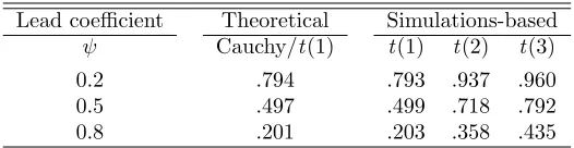
To compare results with Cauchy-distributed processes, Table 1 displays the probabilities of a decrease of at least 25% once the quantile 0.995 is attained for the three distributions and for three distinct lead coefficients. Theoretical probabilities from the same quantile are also reported for Cauchy (t(1)) distributed errors. Simulations-based probabilities differ by a maximum of 0.2% from theoretical results in the t(1) case. Furthermore, recall that the larger the degrees of freedom, the less noisy are estimations for a given number of simulations. That is, we can expect the probabilities for the t(2) and t(3) cases to differ from theoretical probabilities by at most 0.2% and further increasing the number of simulations would lead to more precise results. Given the same quantile, the probabilities of a turning point significantly increases with the degrees of freedom of the distribution and with lower lead coefficients. For the investigated quantile, a process with t(3)-distributed errors and a lead coefficient of 0.2 only has a probability of 4% to keep on increasing as opposed to 20% for Cauchy-distributed processes. Furthermore, simulations indicate that as the series diverges, the probabilities of a crash (impact of the choice of threshold becomes negligible as the modes of the distribution departs from one another) tend to a constant for all models. For a lead coefficient of 0.8 for instance, the probabilities of a downturn tends to 0.2, 0.36 and 0.48 as the bubble increases fort(1),t(2) andt(3) respectively.

Table 1: Probabilities of a crash of at least 25% when quantile 0.995 is attained

Lead coefficient Theoretical Simulations-based

ψ Cauchy/t(1) t(1) t(2) t(3) 0.2 .794 .793 .937 .960 0.5 .497 .499 .718 .792 0.8 .201 .203 .358 .435 Reported probabilities for the simulations-based approach are the av-erage over 1,000 forecasts using 1,000,000 simulations.

tend to a constant during explosive episodes. That is, past some point, the probabilities of a crash will remain constant.

4.2 Predictions using sample-based approximations

This section is based on the approach proposed by Gouri´eroux and Jasiak (2016). They derive a sample-based estimator of the ratio of the predictive densities in Equation (4), which does not always admit closed-form results. Based on past values of the series, this method can also be applied to any non-Gaussian distribution. Whether or not the marginal distributions ofut

and u∗

T+h admit closed-form, they can be expressed as follows,

l(uτ) =Euτ+1

l(uτ|uτ+1),

with τ = {T, T +h}. Once again the noncausal relationship described in Equation (2) is used to evaluate the conditional distribution of l(uτ|uτ+1)

with the distribution of the errors, g(uτ −ψuτ+1). While Lanne, Luoto,

and Saikkonen (2012) employed simulations to approximate expected values, Gouri´eroux and Jasiak (2016) use sample-based counterparts. The expected value here is approximated by the average obtained using all points from the sample for the conditioning variable,

l(uτ) =Euτ+1

g(uτ −ψuτ+1)≈

1

T

T

X

i=1

n

g(uτ −ψui)

o

. (9)

Hence, the predictive density for the MAR(0,1) process ut can be

approxi-mated by plugging the sample counterparts (9) in (4),

l(u∗

T+1, . . . , u ∗

T+h|uT)

≈g(uT −ψu∗T+1). . . g(u ∗

T+h−1−ψu ∗

T+h)

PT

i=1g(u ∗

T+h−ψui)

PT

i=1g(uT −ψui)

. (10)

For centred and symmetrical uni-modal distributions, such as the Cauchy and the Student’s t that are employed in this analysis, the probability density function is maximised at zero. That is, the density g, as it is evaluated in Equation (10), is maximised at the points whereuτ−ψui = 0

as a function of u∗

T+h and will be maximised for paths that were already

undertaken. Furthermore, when uT diverges from all past values in the

sample, the numerator tends to zero, meaning that approximations errors will be amplified during explosive episodes. That is, we can expect this ap-proximation method to put more weight on forecast points corresponding to already undertaken paths and that this tendency will be more pronounced during bubbles.

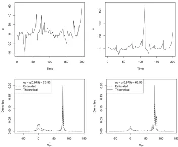
Let us again consider an MAR(0,1) process with a lead coefficient of 0.8 and standard Cauchy-distributed errors. For median levels of the series, results are similar between closed-form and sample-based predictions regardless of past behaviours. However, as the series departs from central values, discrepancies emerge and are path-dependent. To illustrate this, Figure 7 shows one-step ahead density forecasts performed at timeT=200

is needed when building probability-based investment strategies for instance.

Figure 7: Comparison between estimated and theoretical 1-step ahead pre-dictive densities for Cauchy MAR(0,1) with ψ = 0.8 evaluated at quantile 0.975 for 2 distinct trajectories.

due to long lasting bubbles inducing substantial discrepancies between trajectories. This also implies that a larger proportion of points are of higher magnitude, which, as explained above may significantly alter probabilities, hence inducing volatility in the results. The same goes for lower the quantiles, a larger proportion of points of higher magnitude amplifies divergence between probabilities of two distinct trajectories. Increasing the sample size increases the occurrence of extreme episodes which also considerably affect probabilities. Indeed, as we have seen in Figure 7 one previous extreme episode is sufficient to significantly decrease the probabilities of a crash. Furthermore, we can see that the larger the coefficient, the more the sample-based approach tends to overestimates probabilities, compared to theoretical ones (represented by the dotted line). Note however, that the maximum probabilities obtained correspond to the main mode of the distributions and that the divergence of results (resp. the change of quantile) only happen in or (resp. affect) the left tail. Compared to theoretical probabilities, this approach tend to overestimates the probabilities of a crash but results seem to be upper-bounded, and this upper bound corresponds to the most recurrent obtained probability over 1,000 trajectories. However, probabilities of a crash can also be lower than theoretical probabilities, that is, the learning mechanism can indicate that based on past behaviours, the probabilities of turning point are lower than the underlying distribution would suggest.

T=500 T=1000

Figure 8: Distributions of estimated probabilities of a crash of at least 25% for 1,000 different trajectories evaluated at two different quantiles. The dotted lines represent theoretical Cauchy-derived probabilities. The lead coefficient varies (by row) and so does the sample size (by column).

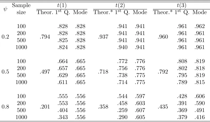
Table 2: Sample-based probabilities of a crash of at least 25% evaluated at Q(0.995) for 1,000 trajectories for each model

ψ Sample t(1) t(2) t(3)

size Theor. 1st

Q. Mode Theor.* 1st

Q. Mode Theor.* 1st

Q. Mode

0.2 100

.794

.828 .828

.937

.941 .941

.960

.961 .962 200 .828 .828 .941 .941 .961 .961 500 .825 .828 .941 .941 .961 .961 1000 .824 .828 .940 .941 .961 .961

0.5 100

.497

.664 .665

.718

.772 .776

.792

.808 .819 200 .657 .665 .756 .776 .802 .818 500 .629 .665 .738 .775 .795 .819 1000 .611 .665 .714 .775 .789 .815

0.8 100

.201

.555 .556

.358

.544 .597

.435

.428 .606 200 .553 .556 .458 .603 .391 .590 500 .404 .556 .259 .607 .369 .491 1000 .343 .556 .290 .605 .379 .416 Theor. corresponds to theoretical probabilities (Theor.* correspond to the probabilities that were derived via simulations in the previous Section reported in Table 1).

Are also reported the 1st_{quantile and the mode of the distribution of the 1,000 probabilities of}

each scenario.

model from which it is easier to simulate. They suggest using a Gaussian

AR model of order s (here an AR(1)) to simulate the process ut. This

approach recovers the intended densities for median levels of the series but fails to recover both the parts corresponding to the crash and to the increase during explosive episodes. The failure of the algorithm for high levels of the series stems from the intention to recover a bi-modal distribution from a uni-modal distribution. If the variance of the uni-modal instrumental distri-bution is not large enough to cover both modes of the sample-based density, the algorithm will not be able to recover the whole conditional distribution. The shape of the Normal distribution significantly depends on past be-haviours of the series since the variance is estimated as the variance of the residuals of the MAR model. Hence, for more volatile series, the variance of the instrumental Normal distribution will be larger, yet, as the variable increases and the two modes diverge, there will always be a point from which the SIR algorithm does not succeed in recovering the density anymore.

the series follows an explosive episode. Indeed, approximations errors amplify with the level of the series, and there is a point from which the SIR algorithm does not recover the whole density anymore. Yet, we find that the sample-based estimator captures the split of the conditional density as the series departs from central values and comprises both the crash and increase parts of the predictive density. Furthermore, it yields time varying probabilities based on its learning mechanism. While sample-based predictive densities based on Student’s t-distributions cannot be compared to closed-form predictions, results corroborate the conclusions drawn with Cauchy. Thinner tails in the errors distribution lead to higher probabilities of crash for given quantiles of an MAR process. A limitation is that when closed-form results are not available, we cannot disentangle how much of the derived probabilities are induced by the underlying distribution and how much by past behaviours. To tackle this, the probabilities estimated with the simulations-based approach of Lanne, Luoto, and Saikkonen (2012) can be used as benchmark as they seem to be good approximation of theoretical results. Such data-driven approach alleviates the issue of constant probabilities that theory or the simulations-based method suggest during explosive episodes. Yet, this is at the costs of heavy computations (increasing with the forecast horizon) and of lack of theoretical guarantees.

5

Empirical Analysis

with locally explosive episodes (that would disappear by taking the returns) we have instead considered the Hodrick-Prescott filtering approach. The detrended series is reported in Figure 9. We are of course aware that this first step might alter the dynamics of the series, probably in the same manner that a X-11 seasonal filter modifies MAR models (see Hecq, Telg, and Lieb, 2017). We leave this important issue for further research. We first estimate an autoregressive model by OLS on the whole HP-detrended Nickel price series. Information criteria (AIC,BIC and HQ) all pick up a pseudo lag length ofp= 2. The three possible MAR(r,s) specifications are consequently anMAR(2,0), anMAR(1,1) or aMAR(0,2). Using the MARX package of Hecq, Lieb, and Telg (2017) an MAR(1,1) with a t-distribution with a degree of freedom of 1.32 and a scale parameter of 347.96 is favoured. The value of the causal and the noncausal parameters are respectively 0.60 and 0.74. We are consequently in the situation in which the predictive density does not admit closed-form expressions (although not very far from the Cauchy) but the sample- and simulations-based approaches can be used.

Figure 9: HP-detrended monthly Nickel prices series. The diamonds rep-resent points from which one-step ahead density forecasts are performed in this analysis.

with settings as close as possible to the assumptions made throughout this paper, we assume the model is correctly specified (parameters estimated over the whole sample) at each point of interest. The points at which we perform predictions are represented by diamonds on the trajectory in Figure 9. We investigate five points along the main explosive episode and one after, to capture the effects of the inclusion of the crash in the predictions. Each point is assigned an index between 1 and 6 indicating their order of arrival. At each point, we compute the sample-based predictive density and compute various probabilities of events (four different magnitudes of crash) derived from both the sample- and simulations-based approaches. Since simulations-based estimations are good approximations (with a large enough number of simulations) of theoretical results, we consider them as theoretical benchmark to which sample-based probabilities are compared.

Results are reported in Table 3. The quantiles corresponding to each of the six points were evaluated using simulations, based on the estimated model, and are presented in the second column. The whole sample up to the points of interest were used in the sample-based approach. For the simulations-based method, given the degrees of freedom estimated for the errors and the quantiles to be investigated, 5,000,000 simulations were employed at each iteration. We investigate the probabilities of a decrease up to 60%. We do not consider larger drops since with a lag coefficient of 0.60, the left mode of the conditional distribution will be located at 60% of the last observed value and, as depicted in the last two columns, the probabilities of larger decrease will quickly decay to zero. Hence, let us now disregard the last two columns for the analysis of the results.

however, as mentioned in Section 4 the choice of threshold may impact probabilities. While this usually concerns the sample-based approach, this is also the case for low quantiles for the simulations-based method as the two modes of the conditional distribution are not sufficiently far to neglect the impact of the choice of threshold. The probabilities of a decrease rose by 1.3% with the sample-based approach between points 4 and 5 while probabilities of a crash of at least 25% declined by 0.1%, due to larger probabilities of drops of lower magnitudes evaluated at point 5.

Point 6 corresponds to a quantile slightly higher than point 2, hence, as expected, theoretical probabilities of a decrease are slightly higher as well. However, as the main explosive episode is now included in the sample-based approximations, the learning mechanism suggests less risk of a crash as the series already departed from such values. This leads to probabilities 12.2% lower than at point 2 for probabilities of a decrease and 9.8% lower for a crash of at least 25%. Furthermore, the discrepancy between the sample-and simulations-based approaches is reduced by more than 11% for both inquiries.

Table 3: One-step ahead probabilities of events for detrended monthly Nickel prices at six different point in time

Point Quantile < yT <75%yT <60%yT <40%yT samp. sims. samp. sims. samp. sims. samp. sims.

1 .518 .291 .147 .227 .116 .185 .097 .131 .075

2 .902 .484 .273 .385 .183 .221 .105 .041 .033

3 .975 .587 .325 .518 .272 .273 .130 .008 .010

4 .984 .591 .330 .539 .289 .294 .139 .004 .006

5 .988 .604 .342 .538 .143 .291 .143 .002 .004

6 .923 .362 .289 .287 .199 .161 .107 .028 .027

The quantiles corresponding to each point were evaluated with simulations based on the esti-mated model.

samp. (resp. sims.) represents sample-based (resp. simulations-based) probabilities. The probabilities are estimated with the following MAR(1,1) model: φ= 0.60,ψ= 0.74 and

t(1.32,347.96) distributed errors.

For the simulations-based approach the following settings were employed: M= 100 and

5.1 Example of investment strategy

Using a monthly series to illustrate investment strategies may not be adequate but this is an example as to how the obtained probabilities could be employed and could be straightforwardly extended to higher frequencies. In addition, while the choice of the de-trending method may alter interpretation, it keeps the locally explosive characteristic of the series and is therefore a good illustrative example. A rather risk averse investor would probably sell once the series reaches point 3, that is when the learning mechanism indicates an increase of the probability of a turning point of 10.3% and more particularly an increase in the probabilities of a drop of at least 25% of 13.3%. Furthermore, as mentioned before, once exceeding all past values, the uncertainty carried by the sample-based approach is translated into a larger discrepancy between the sample- and simulations-based approaches (which then remains rather constant). If this investor did not sell at point 3, they would most likely sell at point 4. At that point, while the learning mechanism does not inflate the probabilities of a turning point (constant discrepancy between the two approaches), it still inflates the probabilities of a drop of at least 25%. This means that going from point 3 to 4, with the same excess probabilities of a turning point, if the series actually drops, higher probabilities are that it will drop by at least 25% when reaching point 4. A more risk seeking investor, if they have not sold yet at point 4 may be misled at point 5, indeed, excess probabilities of a turning point would still be the same that at point 4 while indicating that if the series drops it would less likely drop by more than 25% compared to the previous points. Moreover, any investment strategy using the learning mechanism of the sample-based approach would most probably lead to not selling at point 6 even though the small-scaled bubble crashed the subsequent point. Overall, the extent to which the excess probabilities (discrepancy between the sample- and simulations-based approaches) are used in an investment strategy depends on the beliefs regarding the series. The definition of a crash (namely just a turning point or a drop of at least 25% for instance) depends on the risk aversion of the investor. Further research should be done to investigate more thoroughly structured investment strategies and their performance over larger and diversified data sets.

how much probabilities in the sample-based approach are induced by past behaviours. Indeed, even if probabilities of a turning point were continu-ously increasing with the variable, the discrepancy between probabilities, capturing the variation in uncertainty regarding the downturn may remain constant after some point as we have seen in this empirical example. The two approaches carry different information; on the one hand, the sample-based approach relies heavily on past behaviours and is usually more conserva-tive, yielding higher probabilities of turning points. On the other hand the simulations-based approach yields probabilities solely induced by the un-derlying model. Both methods capture the bi-modality of potential future path characterising locally explosive episodes. They could, individually or combined, be used for investment strategies for instance. However, such strategy depends on what the investor is seeking, their risk aversion and their beliefs regarding the process.

6

Conclusion

This paper analyses and compares in details two approximation methods developed to forecast mixed causal-noncausal autoregressive processes. It focuses on MAR(r,1) processes and aims attention at predictive densities rather than point forecasts as they are more informative, especially in the case of explosive episodes.

the approximations is sufficient and probabilities are also converging to a unique distribution for processes with t(2) and t(3) errors. Both methods capture the bi-modality of the conditional distribution as the series di-verges from central values, which is an indicator of a potential bubble outset.

References

Andrews, B., Davis, R., and Breidt, J. (2006). Maximum likelihood estima-tion for all-pass time series models. Journal of Multivariate Analysis,

97(7), 1638–1659.

Bec, F., Bohn Nielsen, H., and Sa¨ıdi, S. (2019). Mixed causal-noncausal autoregressions: Bimodality issues in estimation and unit root testing

(Tech. Rep.).

Fries, S. (2018). Conditional moments of anticipativeα-stable markov pro-cesses. arXiv preprint arXiv:1805.05397.

Fries, S., and Zako¨ıan, J.-M. (2019). Mixed causal-noncausal AR processes and the modelling of explosive bubbles. Econometric Theory, 1–37. Gouri´eroux, C., Hencic, A., and Jasiak, J. (2018). Forecast performance in

noncausal MAR(1, 1) processes.

Gouri´eroux, C., and Jasiak, J. (2016). Filtering, prediction and simulation methods for noncausal processes. Journal of Time Series Analysis,

37(3), 405–430.

Gouri´eroux, C., and Jasiak, J. (2018). Misspecification of noncausal order in autoregressive processes. Journal of Econometrics,205(1), 226–248. Gouri´eroux, C., Jasiak, J., and Monfort, A. (2016). Stationary bubble

equilibria in rational expectation models. CREST Working Paper. Paris, France: Centre de Recherche en Economie et Statistique. Gouri´eroux, C., and Zako¨ıan, J.-M. (2013). Explosive bubble modelling by

noncausal process. CREST. Paris, France: Centre de Recherche en Economie et Statistique.

Gouri´eroux, C., and Zako¨ıan, J.-M. (2017). Local explosion modelling by non-causal process. Journal of the Royal Statistical Society: Series B (Statistical Methodology),79(3), 737–756.

Hecq, A., Lieb, L., and Telg, S. (2016). Identification of mixed causal-noncausal models in finite samples. Annals of Economics and Statis-tics/Annales d’ ´Economie et de Statistique(123/124), 307–331.

Hecq, A., Lieb, L., and Telg, S. (2017). Simulation, estimation and se-lection of mixed causal-noncausal autoregressive models: The MARX package.

Hecq, A., Telg, S., and Lieb, L. (2017). Do seasonal adjustments induce noncausal dynamics in inflation rates? Econometrics,5(4), 48. Hencic, A., and Gouri´eroux, C. (2015). Noncausal autoregressive model in

Karapanagiotidis, P. (2014). Dynamic modeling of commodity futures prices.MPRA Paper 56805, University Library of Munich, Germany.. Lanne, M., Luoto, J., and Saikkonen, P. (2012). Optimal forecasting of

non-causal autoregressive time series.International Journal of Forecasting,

28(3), 623–631.

Lanne, M., Nyberg, H., and Saarinen, E. (2012). Does noncausality help in forecasting economic time series? Economics Bulletin.

Lanne, M., and Saikkonen, P. (2011). Noncausal autoregressions for eco-nomic time series. Journal of Time Series Econometrics,3(3). Lof, M., and Nyberg, H. (2017). Noncausality and the commodity currency