A diagnostic for the general linear model : an application to Time Series

LEABHARLANN CHOLAISTE NA TRIONOIDE, BAILE ATHA CLIATH TRINITY COLLEGE LIBRARY DUBLIN

OUscoil Atha Cliath The University of Dublin

Terms and Conditions of Use of Digitised Theses from Trinity College Library Dublin Copyright statement

All material supplied by Trinity College Library is protected by copyright (under the Copyright and Related Rights Act, 2000 as amended) and other relevant Intellectual Property Rights. By accessing and using a Digitised Thesis from Trinity College Library you acknowledge that all Intellectual Property Rights in any Works supplied are the sole and exclusive property of the copyright and/or other I PR holder. Specific copyright holders may not be explicitly identified. Use of materials from other sources within a thesis should not be construed as a claim over them.

A non-exclusive, non-transferable licence is hereby granted to those using or reproducing, in whole or in part, the material for valid purposes, providing the copyright owners are acknowledged using the normal conventions. Where specific permission to use material is required, this is identified and such permission must be sought from the copyright holder or agency cited.

Liability statement

By using a Digitised Thesis, I accept that Trinity College Dublin bears no legal responsibility for the accuracy, legality or comprehensiveness of materials contained within the thesis, and that Trinity College Dublin accepts no liability for indirect, consequential, or incidental, damages or losses arising from use of the thesis for whatever reason. Information located in a thesis may be subject to specific use constraints, details of which may not be explicitly described. It is the responsibility of potential and actual users to be aware of such constraints and to abide by them. By making use of material from a digitised thesis, you accept these copyright and disclaimer provisions. Where it is brought to the attention of Trinity College Library that there may be a breach of copyright or other restraint, it is the policy to withdraw or take down access to a thesis while the issue is being resolved.

Access Agreement

By using a Digitised Thesis from Trinity College Library you are bound by the following Terms & Conditions. Please read them carefully.

A Diagnostic for th e General Linear Model

An Application to Time Series

by

Carl Sullivan

Thesis submitted for the degree of Doctor of Philisophy

Department of Statistics

Trinity College Dublin

Supervisor: Prof. John Haslett,

Department of Statistics, Trinity College Dublin

D ecla ra tio n

This thesis is entirely the author’s own work. The contents of this thesis have

not been subm itted as an exercise for a degree at any other University. The

contents of this thesis may be lent or copied without the author’s consent by

the Library at Trinity College Dublin.

Signature of A uthor

Sum m ary

An outlier is an observation which is thought to be unusual. The detection

of such extreme values is an important issue. Developing a model based on

data containing even a single outlier can seriously bias population inferences.

The valuable role marginal and conditional residuals play in assuring model

robustness is well established in the context of general linear models. The

purpose of this thesis is to explore the potential of a statistic, developed

for general linear models which incorporates both marginal and conditional

residuals, as a diagnostic tool for time series and longitudinal data.

Theory is developed which enables this statistic to be applied in a wider

range of situations. Empirical evidence is presented which displays the di­

agnostic’s ability at detecting a wide variety of aberrant behaviour in times

series. Particular attention is paid to single outliers and groups of outlying

points. These methods generalize for multi-dimensional variables. Detecting

influential observations is examined as well.

A cknow ledgem ents

I would like to thank my parents for encouraging my pursuit of knowledge

and I promise to get a job soon. A special thanks to my supervisor, John

Haslett, for all his tim e and enthusiasm.

Thanks Deazer for being a friend and p u tting up with my thursday rants.

Thanks for the camping experience Vince. I ’d like to thank Cassian for all

the games of pool and snooker, and yes I’m in the lead frame-wise. Thanks

for the raindeer m eat and the Finnish vodka Niko. Rome was great and

Teramo was even b etter thanks Aldo (My Master). Greek culture seems sur­

prisingly similar to Irish culture someday Georgos I will make it to Greece.

Thanks G ilbert and Jan for the experience th a t was Keele University and of

course the fine English Ales as well. Finally, I’d like to thank Cathal, Clare,

Breedette, Ronnie, Pete, Eoin, Ingelin and Eleisa for making postgraduate

life a little more interesting.

C ontents

1 In tro d u ctio n

1

1.1 Summary of re s e a rc h ...

1

1.2 Extensions in Original F i e l d ...

2

1.3 Computationally Cheap A pproxim ations...

3

1.4 Application to Time S e rie s...

4

1.5 Diagnostics for Longitudinal D a t a ...

5

1.6 Mahalanobis Distance A pproach...

5

2 C on trib u tion M eth o d o lo g y

7

2.1 Outlier Diagnostic ...

7

2.2 Residuals ...

8

2.2.1

Marginal R e sid u a ls...

8

2.2.2

Conditional Residuals ... 10

2.3 C o n trib u tio n s... 11

2.5

A p p licatio n s... 14

2.5.1

Contributions and Simple Linear M o d e ls ... 15

2.5.2

Contributions and General Linear Models ... 20

2.6

Unusual Negative C o n trib u tio n s... 23

2.6.1

Upper B o u n d ...

23

2.6.2

Lower B o u n d ... 24

2.6.3

Application of B o u n d s ... 25

2.7 General Linear Models to Time S eries...27

3 A pproxim ating Standardized Contributions

28

3.1

Com putational Efficiency... 28

3.2

Influence and R a n g e s ... 29

3.3

S u b se ts... 33

3.4

Fixed effects are k n o w n ...36

3.5

Fixed effects are u n k n o w n ... 40

3.5.1

Independent O b s e rv a tio n s ... 40

3.5.2

General Covariance S t r u c t u r e ... 44

3.6

A Cheap Approximation of

...48

3.7

C o n c lu s io n s ...50

4.2

Prediction Error D eco m p o sitio n ...53

4.3

Time Series Diagnostic R ev iew ...57

4.3.1 Reviewing D V ( A ) ... 58

4.3.2 Likelihood Ratio ...

4.3.3 Leave-K/i-Out D ia g n o s tic s ... 60

4.4 A Single O u tlie r... 62

4.4.1 An Additive O utlier ... 62

4.4.2 An Innovative Outlier ...

4.5

Subsets of Unusual O bservations... 71

4.6

Level

S h i f t s ...76

4.7

C o n c lu sio n s...80

5 L on gitu d inal M odels

81

5.1

Laird-Ware M o d e ls ... 81

5.2

Random E ffe c ts ...82

5.2.1

Outlying O b s e rv a tio n s ... 83

5.2.2

Outlying I n d iv id u a ls ...

5.3

Random Effects and

AR{1) E rro rs ...

5.4

C o n c lu sio n s...

6.2

Mahalanobis Distance

... 98

6.3

Additive P ro p e rty ... 99

6.4

Application of M i S ta tis tic ...100

6.4.1

Single Outliers

...100

6.4.2

Groups of O u t l i e r s ...101

6.5

C o n c lu sio n s...106

7 Further R esearch

107

7.1

Possible Theoretical E x te n s io n s ... 107

7.2

C o n c lu s io n s ... 108

A p p en d ices

A A d d itio n a l P ro o fs

109

A .l Propositions used in C hapter 2

109

A.2 Compound Symmetry and

...114

A.3

for Experimental U n i t s ...116

B G eneral Form o f

118

B .l Covariance of

and e(^)

... 118

List o f Tables

2.1 Analysis of Forbes’ D a t a ... 16

2.2 Analysis of Huber’s D a t a ... 18

2.3 Analysis o f Ice-cream D a t a ... 22

2.4 Negative Contributions of Ice-cream d a t a ...26

3.1

and

7^ associated with Forbes’ D a t a ... 43

3.2

and

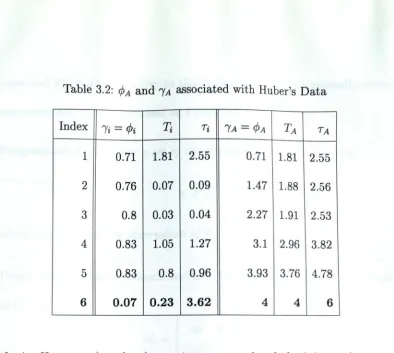
associated with Huber’s D a t a ...44

4.1 Diagnostic Results for a Single Additive O u t l i e r ...65

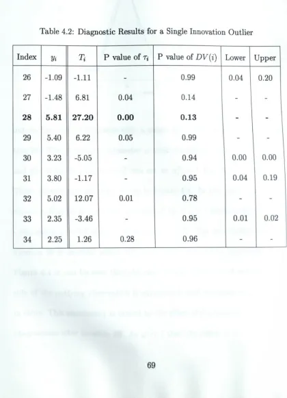
4.2 Diagnostic Results for a Single Innovation O u t lie r ... 69

4.3 Diagnostic Results for a Patch of Additive O u t l i e r s ...73

4.4 Unusual Contributions for Nile D a t a ...78

5.1 Contributions for Individual with Single Outlying Observation

85

5.2 Contributions for Outlying In d iv id u a l... 88

5.3 Observations with UnusuaJ Contributions in Zerbe’s D ata . . . 91

5.4

Unusual Standardized Residuals of Observations associated

with Outlying I n d iv i d u a ls ... 93

6.2 Mi Analysis of a Single ^novation Outlier

6.3 M, Analysis of a Patch of Additive Outliers

6.4 Unusual Mi values for Nile D a ta ...

List o f Figures

2.1 Forbes’ D a ta ... 15

2.2 Huber’s D a t a ... 18

2.3 Ice-cream D a t a ...21

3.1

(j)A

and

associated with AR{1) processes...39

3.2

(j)A

and

associated with Ice-cream D a t a ... 47

3.3

T

and

associated with Ice-cream D a t a ... 47

3.4

T

and

associated with Ice-cream D a t a ... 50

4.1

Single Additive O u tlie r... 63

4.2 Rate of Detection for An Additive O u t l i e r ...65

4.3 Single Innovation O u tlie r... 68

4.4 Rate of Detection for An Innovation O u tli e r ...70

4.5 Patch of Additive O u tlie rs... 72

4.6 Rate of Detection for a Patch of Additive O u tliers...74

4.7 Rate of Detection for a Patch of Additive Outliers using

DV{i) 75

4.8

Annual Flow Volume of

the N ile ...76

4.10 Level Shift Diagnostics with the year 1913 O m i t t e d ...79

5.1

Single Outlying O b se rv a tio n ...

5.2

Single Outlying I n d iv id u a l... ...

5.3 Zerbe’s D a t a ... gg

5.4

Expected Plasma Inorganic P h o s p h a te ...

5.5

versus

for In d iv id u a ls ...

5.6

and

associated w ith an I n d iv id u a l...

5.7

and

associated with an I n d iv id u a l...

6.1

P values of M(^a

105

C hapter 1

In trod u ction

1.1

Sum m ary o f research

Detecting and explaining observations th a t are outlying has generated con­

siderable m aterial in books and journals. New developments in theory and

application are continuously occurring. The detection of outliers continues

to remain an im portant issue. As new models are developed and applied,

an understanding of their robustness and sensitivity to unusual observations

is im portant. A single outlier or ju st a small subset of unusual observations

may greatly influence the inferences made about the entire population. Out­

liers may also provide evidence of model inadequacies.

This thesis focuses on th e viability of using a statistic, developed for gen­

in tim e series and longitudinal data. Theoretical developm ents presented in this thesis allows th e application o f this statistic to a wider range o f situa­ tions. Empirical evidence leads to th e development of com putationally cheap approxim ations and bounds for th is diagnostic.

This statistic is referred to as the c o n trib u tio n of a single datum or

collection of data points to the lack of fit. The contribution statistic has

an additive property, detailed in chapter 2, which makes it highly computa­

tionally efficient compared to existing diagnostics. Remarkably this additive

property is valid even when observations are correlated such as those com­

mon to time series and longitudinal data. It is this property which instigated

the research contained in this thesis.

1.2

E x ten sio n s in O riginal F ield

Chapter 2 of this thesis defines, explores and extends this statistic in its

original field of development. In the case of simple linear models,

~

N{X/3,a'^I), the relationship between internally studentized residuals and

the standardized version of this statistic is established. Clearly, in this case,

the standardized contributions have a simple and easily interpretable mean­

ing. The contributions and their standardized versions are always positive if

Y

N{Xl3,a^I).

When y

N{ X/ 3, V)

the contributions and the standardized contribu­

tions may take negative values. Considerable effort is spent in Haslett and

Hayes [29] to show how unusual observations can be detected by examining

the contributions of the data points to the lack of fit. However all of these

unusual observations generate large positive contributions. The authors were

unable to establish what information lies in the negative tail of the contri­

butions’ distributions. Indeed, no methods were even proposed to detect

unusually large negative contributions.

The problem of large negative contributions is first detailed in chapter

2. Empirical evidence in chapter 4 indicates a type of outlier found in time

series that can generate large negative contributions. Theory is developed

in chapter 2 to enable the detection of unusual observations which gener­

ate unusually large negative contributions. These theoretical developments

make the contribution diagnostics a far more comprehensive methodology for

outlier detection.

1.3

C om p u tation ally Cheap A pproxim ations

increases. To standardize a contribution two parameters must be evaluated.

One parameter is computationally cheaper than the other hence it is more

desirable to work with this easily obtained parameter if possible.

Chapter 3 focuses on the relationship between these two parameters. The­

ory is derived which establishes when both these parameters are equal. Em­

pirical evidence suggests situations when they are approximately the same.

Their relationship to subset size is also explored. As a result of this analysis

the conditions under which the contributions are themselves good approxi­

mations of their standardized versions are established. For cases when the

contributions differ greatly from their standardized contributions computa­

tionally cheap approximations are proposed.

1.4

A p p lication to T im e Series

Serial correlation is fundamental to time series, hence any diagnostics applied

to these series must be able to utilize the correlation structure. Haslett and

Hayes [29] go to great lengths to emphasize the ability of the contribution

methodology to detect outliers when observations are correlated; in fact all

the examples presented in their paper assume non-independence. These ex­

amples along with the examples and theory in chapter 2 justify exploring the

contribution approach with respect to time series analysis.

Chapter 4 reviews existing diagnostics in time series analysis and com­

pares then to the contribution approach. Empirical evidence illustrates the

ability of contribution diagnostics at detecting additive and innovation out­

liers, see Fox [23]. The detect of unusual subsets and level shifts are also

explored.

1.5

D iagnostics for Longitudinal D ata

The contribution methodology is applied to longitudinal data in chapter 5. A

very general class of models is considered in Chi and Reinsel [10] which allow

for fixed effects, random effects and for the errors to have a serial correlation

structure. Empirical evidence is presented of the standardized contribution

diagnostic’s ability at detecting both outlying observations and individuals

for such models. The data set analyzed in Chi and Reinsel [10] provides

further empirical evidence of the accuracy of the computationally cheap ap­

proximations put forward in chapter 3 for the standardized contributions.

1.6

M ahalanobis D istan ce A pproach

generate the contributions. This statistic is geometrically more interpretive

then the contribution approach. Its relationship to the contribution statistic

is theoretical established.

Examples are presented which illustrates the ability of this new diagnostic

at detecting a range of unusual behaviour experience by time series. This

diagnostic is not as com putationally efficient as the contribution approach

and numerical difficulties can arise due to singular covariance matrices.

C hapter 2

C ontribution M ethodology

2.1

O utlier D iagn ostic

large negative contributions. These new developments aid in the intrepreta-

tion and range of applications of the contribution methodology.

2.2

R esiduals

The concept of a residual is fundamental to applied statistics. In its simplest

form it can be defined as:

residual = observation — fitted value.

Given a set of observations

Y

and a set of estimates

Y

for these observations

the vector of residuals are given by

Y - Y .

Clearly the values of the residuals

depends on how

Y

was obtained. Thus different estimates of

Y

will generate

different residuals. By examining residuals the appropriateness of models

can be assessed, the strength of underlying assumptions of normality or ho-

moscedasicity can be gauged and outlying observations can be detected.

Two different types of residuals are used to construct the contribution

statistic and they are referred to as marginal and conditional residuals. Both

these residuals are reviewed in the following subsections.

2.2.1

M arginal R esid u als

Given a set of observations

Y

N(XP, V) ,

where /3 and

V

are known then

the set of marginal residuals are defined as e = y —

E[Y] = Y — X

The

marginal residual associated with the data point

i

is denoted Cj and

C

responds to the marginal residuals of the set of observations

A.

In many situations

/3,

commonly referred to as the fixed effects of the

model, is unknown and has to be estimated. The marginal residuals are

now defined

as e = Y - X $

where ^ is an estimate for the unknown pa­

rameter

p.

For generad linear models the classical estimate for

is given by

p = { x ' ^ v - ^ x y ^ x ' ^ v - ^ Y =

B y.

It is also common for the covariance matrix of Y, denoted

V,

to be un­

known. The covariance matrix

V

can be written as V =

a'^R{Q)

where cr^

is associated with the variance of individual components of

Y

and H(0) de­

scribes the correlation structure associated with

Y.

For general linear models

the classical estimate for

is given by

=

e^R{Q)~^e/{n—p)

where p is the

rank of

X

and

n

is the number of observations in

Y.

The correlation param­

eters used to construct

R{Q)

are denoted by 0 and if they are unknown they

can be estimated by maximum likelihood or restricted maximum likelihood.

For the moment, it is assumed

V

is known or an estimate is available. In

this chapter, the covariance matrix

V

or its estimate will simply be referred

to as

V.

as

The variance of a single marginal residual

is

given by the

diagonal element of the matrix

hence

The

variance of

follows and is given by

G a a

=

var[e/^. This representation

can be found in Haslett and Hayes [29].

2.2.2

Conditional R esiduals

The conditional residual, e(j), for an observation

yi is defined as:

6(0 = I/i - y(i)

where y(j) =

E[yi\yi-,

V]. y^i) is the best linear unbiased predictor (BLUP),

see Robinson [49], of yi given the observations y; = (t/i,. . . ,

j/ii, . . . , y n )

-P^i) is used to denote the estim ate o f the fixed effects

P om itting the obser­

vation

yi. However the estim ate o f the variance structure

V

is based on the

entire data set. The conditional residuals associated w ith a subset A is given

by:

= y A - V{A)

where y(^) =

E[yA\yA\ P(,A)ty]- The expected value o f the conditional resid­

uals is zero and their variance is

=

see H aslett and Hayes [29].

The following formula

shows the relationship between the marginal and conditional residuals. It

is interesting to note that Haslett and Hayes [29] showed this relationship

in the context of general linear models and that de Jong and Penzer [18]

proved it in a time series context. In time series analysis it is common

for the conditional residual to be referred to as a cross-validation residual,

see Christensen [11] section 2.2, or as a leave-«^-out residual in Bruce and

Martin [8]. However, leave-/Cyi-out residuals as defined in Bruce and Martin

[8] involve the re-estimation of the covariance structure with

observations

removed whereas in this thesis

V

is not re-estimated.

2.3

C ontributions

The contributions arise from the decomposition of the lack of fit which is

denoted

S

and is defined

as S = {Y — X 0 ) V~^{y — X 0 )

=

e^V~^e.

It is

possible to express

S

in terms of both maurginal and conditional residueds

S = f: r f r 'e ,e n ,= f ; T ,

i = l »=1

I

= { l , 2 , . . . , n } denote the indexing set. For time series a n a tu ral indexing

set exits, however for general linear models an artificial indexing m ay have

to be defined.

I

maybe partitioned into an arbitrary number of subsets,

I

=

{ A i , A

,

Ar} of dimensions «i,/Ca, • • • , such that n=X)i=i

and

Ki < n - p for all z. This p artitioning of the indexing set allows the lack of

fit to be expressed as follows

s = i: T A .

i=l

where

T

^

=

is referred to as the contribution of the data

subset A i to the lack of fit 5. T h e contribution Ta, of an arbitrary subset A,

can be expressed as

ieA

which is a sum m ation of the individual contributions of each d atu m indexed

by the set

A . Thus the contributions of any subset can be obtained by adding

the contributions of each datum in the subset. Thus th e contribution for any

a rb itrary subset can be generated with com putational ease.

H aslett and Hayes [29] show th a t the contribution of a subset

A

can be

expressed as follows

+

(

7

-

-

2

^

' ^

contri-butions E \T

=

see H aslett and Hayes

[29]. The variance of the contributions is given by

=

and

is defined as follows

74 = tr{(GLoj'GL)'} = E ’f.’

1 1

where TTj are the eigenvalues of F =

^^e Haslett and Hayes [29].

The properties of 4>

Although the expected value of T

and its variance are available, calcu­

lating

by simulation or numerical approxim ation methods, see M athai and Provost

[41]. However, this representation of contributions allows the application of a

transform ation found in M athai and Provost [41], section 4.6, which enables

to be standardized to an approxim ately

random variable. This new

statistic is referred to as the standardized contribution.

2.4

Standardized C ontributions

is denoted

and is defined as

f

{T

- 4>

)V ^

, ,

where

=

and

var{rA)

=

2

Ta

approximately

distributed.

Unfortunately the standardizing contribution

does not share the same

additive property as

thus

t a

/

Y.T'i-i €A

As a result generating

requires a lot more computations then

-2.5

A pplications

Three d a ta sets are examined in this section. A simple linear model is as­

sumed for two of these d ata sets while a general linear model is applied to

th e third. All the models require the estim ation of two fixed effects: an in­

tercept and a slope. Each of these examples contains only one outlier which

is represented graphically by the symbol 0 . However each outlier provides

its own unique challenge. Leverage is not an issue for Forbes’ d a ta which

be-Figure 2.1: Forbes’ Data

■2135

196

- r

201 206

X « boiling p o in t ( ° F )

tween observations. The ability of the contributions to detect these unusual

observations with this variety of challenges is shown.

2.5.1

C ontributions and Sim ple Linear M odels

It is assumed in this subsection that

Y

~

N{XP,a"^I).

The first data set to

be examined is Forbes’ data amd is displayed in Figure 2.1. This data set was

collected in the 1840s and 1850s by James D. Forbes, see Weisberg [50], and

was used to estimate altitude by understanding the relationship between the

Table 2.1; Analysis of Forbes’ Data

Index

Ti

6(i)

A

1

131.79

194.5

0.42

0.53

-0.25

-0.31

0.19

0.33

2

131.79

194.3

0.03

0.04

-0.07

-0.08

0.20

0.02

3

135.02

197.9

0.03

0.03

-0.06

-0.07

0.11

0.02

4

135.55

198.4

0.00

0.00

0.02

0.02

0.10

0.00

5

136.46

199.4

0.01

0.01

0.04

0.04

0.08

0.01

6

136.83

199.9

0.01

0.01

-0.04

-0.05

0.08

0.01

7

137.82

200.9

0.02

0.02

0.05

0.06

0.07

0.01

8

138.00

201.1

0.02

0.02

0.05

0.06

0.07

0.01

9

138.06

201.4

0.17

0.18

-0.16

-0.17

0.06

0.10

10

138.05

201.3

0.04

0.04

-0.08

-0.08

0.06

0.02

11

140.04

203.6

0.15

0.16

-0.15

-0.15

0.06

0.08

12

1 4 2 .3 4

2 0 4 .6

1 2 .8 7

1 3 .7 5

1 .3 6

1 .4 5

0 .0 6

7 .3 4

13

145.47

209.5

0.00

0.00

0.00

0.00

0.14

0.00

14

144.34

208.6

0.73

0.82

-0.32

-0.37

0.12

0.47

15

146.30

210.7

0.41

0.50

-0.24

-0.29

0.17

0.30

16

147.54

211.9

0.04

0.05

-0.08

1

o

o

0.21

0.03

17

147.80

212.2

0.05

0.07

-0.09

-0.11

0.22

0.04

of introducing the concept of simple linear regression. The Forbes’ d a ta is

used in Atkinson [2] to illustrate the detection and effects of an outlier on

simple linear models. Observation 12 of this data is deemed to be unusual in

Atkinson [2]. Prom Table 2.1 it is clear th a t the contribution associated with

this observation is extremely large compared to the contributions generated

by the other d ata points. The standardized contributions provides further

evidence th at observation 12 is outlying. Cook’s distance denoted

Cook [13], reveals th a t this d atu m is adso influential in the estimation of the

fixed effects. The leverage of th e

observation is denoted

and from

Table 2.1 it is clear no observation has an unusually large leverage.

The next d a ta set explored is H uber’s d a ta and is displayed in Figure

2.2.

This d ata is a synthetic exam ple used in Huber [30] to illustrate

the effects of points with high leverage on model selection and param eter

estim ation. This example differs from any application presented in Haslett

and Hayes [29] as th e issue of leverage arises. Cook’s distance generates an

exceptionally large vaJue for observation 6, see Table 2.2. It is interesting

to note th a t the contribution associated with this d atu m does not appear

unusual when contrasted with the contributions of th e o ther d a ta points.

However its standardized contribution indicates th a t this point is

W hat causes this dram atic difference?

Figure 2.2: Huber’s Data

2

1

0

■1

2

-5.5 -3.0 -0.5 ZO _{4.5 7.0 9.5}

X

Table 2.2: Analysis of Huber’s Data

Index

6(0

A

1

2.48

-4

1.81

2.55

2.09

2.94

0.29

1.79

2

0.73

-3

0.07

0.09

0.42

0.55

0.24

0.06

3

-0.04

-2

0.03

0.04

-0.27

-0.34

0.20

0.02

4

-1.44

-1

1.05

1.27

-1.59

-1.93

0.17

0.77

5

-1.32

₀

0.8

0.96

-1.39

-1.67

0.17

0.58

6

0.00

10

0.23

3.62

0.75

11.64

0.93

28.21

Hayes [29] state that when

Y

N{XP,a'^I)

then the contributions of an

arbitrary subset indexed by

A

can be expressed as

i&A ^

The authors failed to simplify the standardized contributions. When

V = d^I

then it follows, see Appendix A. 1.3, th at the standardized contribution of an

arbitrary observation can be expressed as

r =

-‘ <72(1 - / I , , )

where

ha

is the leverage of the

d ata point. Thus Tj, in this case, can be

viewed as an internally studentized residual which is squared, see Atkinson

[2]. This allows the Cook’s distance corresponding to this observation to be

expressed as

A =

p (l -

ha)

where

p

is the rank of the design matrix. In this situation, the Cook’s dis­

tance of a single observation is a scalar multiple of r^. The standardized

contribution of a subset of observations. A, can be expressed as

=

e?

_

see Appendix A. 1.4.

their standardized versions when leverage is an issue. It is also worth noting

that both

T

.

and

depend on the square of the marginal residuals and this

is the reason they can never be negative when

y ^ N{Xl3,a'^I).

2.5.2

C ontributions and G eneral Linear M odels

It is assumed in this subsection that

Y

~

N{XP,V).

The Ice-cream data set

is displayed in Figure 2.3. This data set was collected in the 1950s in America

and was used to explore the relationship between ice-cream consumption and

such factors as weekly family income, the price of ice-cream and monthly

mean temperatures, see Kadiyala [34], A detailed analysis of this data is

performed in Martin [40] with an emphasis on outlier detection. The same

model is used for the analysis now performed on the Ice-cream data as that

proposed in Martin [40]. This model was selected by Martin [40] on the

grounds of parsimony and fit. The data is modeled with a straight line

regression on the mean temperature and the errors, Ct, are assume to be

from an autoregressive process of order one

g{ = <pet-i + £t

where

(p —

0.75 and

= 0.00105, see Diggle [21] section 2.4 for an intro­

duction of autoregressive processes.

Figure 2.3: Ice-cream Data

c 0.51

-*2.

c 0.41

0.31

0.21 ---1---1--- r

20 30 40 50

X » Temperature ( “F )

60 70

seen in Table 2.3 that this observation has both an exceptionally high con­

tribution and standardized contribution. This point is not influential, in fact

there are no influential observations present in this data set. Leverage is not

an issue.

W hat makes this d ata set different from the previous two examples is that

some of the contributions Jtad indeed some standardized contributions are

negative. Haslett and Hayes [29] note th at negative contributions may occur

when observations are assumed to be correlated. However, they remain un­

Table 2.3: Analysis of Ice-cream

Data

Index

^ ii) h i i

A

1

0.39

41

1.89

1.99

0.04

0.06

0.11

0.19

2

0.37

56

0.87

0.94

-0.02

-0.03

0.02

0.01

3

0.39

63

0.36

0.56

-0.02

-0.01

0.00

0.00

4

0.43

68

-0.20

0.14

-0.01

0.02

0.01

0.00

5

0.41

69

-0.53

-0.11

-0.03

0.01

0.01

0.00

6

0.34

65

2.92

2.44

-0.08

-0.02

0.00

0.00

7

0.33

61

0.95

1.01

-0.08

-0.01

0.03

0.00

8

0.29

47

1.69

1.52

-0.08

-0.01

0.00

0.00

9

0.27

32

-0.42

-0.02

-0.05

0.01

0.02

0.00

10

0.26

24

0.27

0.53

-0.04

-0.00

0.05

0.00

11

0.29

28

0.04

0.27

-0.02

-0.00

0.01

0.00

12

0.30

26

-0.02

0.28

-0.00

0.00

0.03

0.00

13

0.33

32

0.28

0.50

0.01

0.02

0.00

0.00

14

0.32

40

1.09

1.10

-0.03

-0.03

0.02

0.01

15

0.38

55

-0.32

0.07

-0.01

0.02

0.02

0.00

16

0.38

63

2.28

1.96

-0.04

-0.04

0.00

0.00

17

0.47

72

1.65

1.59

0.03

0.04

0.03

0.03

18

0.44

72

-0.02

0.28

-0.00

0.01

0.01

0.00

19

0.39

67

0.70

0.81

-0.04

-0.01

0.00

0.00

20

0.34

60

2.55

2.19

-0.07

-0.03

0.03

0.01

21

0.32

44

-0.64

-0.17

-0.04

0.01

0.04

0.00

22

0.31

40

0.13

0.38

-0.04

-0.00

0.00

0.00

23

0.28

32

1.56

1.46

-0.04

-0.03

0.01

0.00

24

0.33

27

1.16

1.20

0.02

0.04

0.02

0.01

25

0.31

28

-0.01

0.28

0.00

-0.03

0.01

0.00

26

0.36

33

1.13

1.14

0.03

0.02

0.01

0.00

27

0.38

41

-0.22

0.13

0.03

-0.01

0.01

0.00

28

0.42

52

0.59

0.72

0.03

0.01

0.00

0.00

29

0.44

64

-1.28

-0.66

0.02

-0.05

0.01

0.01

There are ten negative contributions in Table 2.3 so one third of the data

generate negative contributions. Observation 29 appears to have a large neg­

ative contribution compared to the other negative values. Concerns about

observation 29 are mentioned in M artin [40] due to this datum generating a

large negative studentized residual, approximately -2. Thus a large negative

contribution appears to indicate a departure from the model. The detection

of observations which generate large negative contributions is considered in

the next section.

2.6

Unusual N egative Contributions

Calculating

P(T

< —t)

where

T

is the contribution of an arbitrary subset

indexed by

A

and i is a positive real number can only be achieved by sim­

ulations or numerical approximation methods, see section 2.2. A method is

proposed, in this section, of detecting unusually large negative contributions

by obtaining upper and lower bounds for P(T^ <

—t).

These bounds can be

easily generated.

2.6.1

U p p er B ound

The following proposition shows how an upper bound for

P{T

< “ 0

P r o p o sitio n 2.6.1

L e t t e d such that t >

0

then

P ( T

< - * ) < ! -

P { ^ <

- ^

)

1a-4>a

where a; ~ y? .

P r o o f By definition

where

~

and

~

definition

7

^ > 0 and

> 0. It

follows th a t if

<

then

P(r,<-*) =

p C - ^ n - ^ - ^ v . < - t )

< p (_ i2 iL z M u 2 <

- t )

2k a

Df

\

=

=

\-p {v ,< :^ ^ ).

I

- 0/4

2.6.2

Lower B ound

The following proposition gives a lower bound for

<

Unfortu­

nately this lower bound is only valid for subsets of size one or two. Finding

lower bounds for subsets greater th an two is an area of current research.

P r o p o s i t i o n 2 .6 .2

0

P (T a

< - * ) > ! - P ( i <

where x

~

= 1 or

=

2.

P r o o f Let

Vi

~

xl^

and

V

~ x L

definition

P { T A < - t ) =

Let

/ N nC 7/1 “ <^>1 ^ + 7/1 + ^

note

g{v\)

is a convex function when /c^ = 1 or

= 2, see appendix A.1.1.

Hence

>

by Jensen’s Inequedity, see Mood

et al.

[43]

r>f 7/1 ^ , 7/1 "t” 171 r i\

= P(„,>

+

7/1 - <P A J A - 4>A

1 n / ^ 2 i/t/i 7 a + 4* A n

2.6.3

A p p lication of Bounds

These bounds are used to exam ine the negative contributions generated by

Table 2.4: Negative Contributions of Ice-cream d a ta

Index

Ti

Lower Bound

Upper Bound

4

-0.20

0.04

0.45

5

-0.53

0.02

0.21

9

-0.42

0.03

0.27

12

-0.02

0.05

0.82

15

-0.32

0.03

0.35

18

-0.02

0.05

0.83

21

-0.64

0.02

0.18

25

-0.01

0.05

0.84

27

-0.22

0.04

0.43

29

-1.28

0.01

0.06

values increase in m agnitude the difference between the bounds decreases.

In fact V

€ { 1 ,2 ,3 ,...}

lim

t-foo _{l A - < l > A l A - (l>A} -

P{v. <

II

0

T he probability of observing a negative contribution of larger

than observation 29 is between 0.01 and 0.06. This range indicates that

although the contribution of observation 29 is n ot exceptionally

there is still some evidence th a t observation 29 deviates from the

When the Ice-Cream data is re-analyzed with the outlying observation 30

omitted then observation 29 generates a positive contribution close to zero.

In Martin [40] when the analysis is redone with observation 30 removed then

observation 29 generates a positive studentized residual close to zero. This

shows th at contributions can suffer from sm earing, see Bruce and Martin

[8], where smearing is used to define non-outlying observations being detected

as outlying due to the influence of outlying points elsewhere.

2.7

G eneral Linear M od els to T im e Series

Each unusual observation in the three data sets was detected by the stan­

dardized contributions. These examples provide further empirical evidence

of the ability of this approach at detecting unusual observations in simple

and general lineaj models.

The success of this method to detect outlying points in the presence of

high serial correlation opens the way forward to application in the field of

time series analysis. It is now possible to detect unusually large negative con­

tributions. The importance of this development with respect to time series

analysis is explored in chapter 4. It has also been established th at contribu­

tions and standardized contributions suffer from smearing so care must be

Chapter 3

A pp roxim atin g Standardized

C ontributions

3.1

C om putational E fficiency

The additive property of the contributions,

makes them more

desirable to work w ith from a com putational view point th an their non­

additive standardized versions. Thus for com putational efficiency it would

be very useful to know when

is a good approxim ation for

The rela­

tionship between

and

is determ ined by the param eters

and

It

is these param eters which indicate the models for which

is a good approx­

im ation for

and for which it is not. W hen

is not a good

com putationally cheap approxim ation.

Except for models where observations are assumed to be independent, the

param eter 74 is computationally more difficult to obtain then the param eter

4

thus

correspond­

ing to the observations in the set

The param eter 7^ does not share this

additive property except when observations are assumed to be independent;

w ithout this assumption there appears to be no simple relationship between

74 and {7i|i e A}. However this chapter provides evidence th a t in many

situations

is a good approxim ation for

the p value associated w ith

to be used as a bound for the p value of

ta-The following sections in this chapter focus on the param eters

and 7^.

Theoretical exploration, along w ith com putations of these param eters, gives

insight into the relationship between

and

T he result of this work is

com putationally cheap approxim ations and bounds for

based on

3.2

Influence and R anges

For observations where homoscedasicity is assumed

and

are

dent of the variance of the observations. It is the correlation structure of

the values taken by

and

>i. This can easily be seen in th e case of the

param eter

^; by definition

= tr({I - X { X - ^ R - ' X ) - ' x ' ^ R - \ ^ )

since

V = a“

^R,

where H is a correlation m atrix. It can be shown in a similar

m anner th at

is independent of the variance of observations. If the vari­

ance of the d a ta is not constant then the param eters

and

will both be

influenced by the variance of the observations.

The ranges of the param eters

4>

and

^ will now be defined. From

proposition 3.2.1 it is established th a t, for any general linear model, the pa­

ram eter

<I)A

has a limited range from zero to

-

Proposition 3.2.2 proves

th a t

> 0- The example after proposition 3.2.2 provides evidence th at any

upper bound of

would depend on the correlation stru ctu re of the obser­

vations. From the example presented in this section a correlation structure

can be constructed such th a t

^ is exceptionally large. As a result

T

has

the potential to be very different from

-P r o p o s it io n 3 .2 .1

The param eter (f>i has the following range

0 < ( f > i < l .

In the general case

has the following range

0 < ( p A < l i A

where

is the size of the subset A.

P r o o f

By definition

<!>< = {VQ)u

where

VQ = I - X{ X' ^ V - ^ X ) ~ ^ X ' ^ V - ^ = I - H .

Both

VQ

and

H

are idempotent matrices. Idempotent matrices have eigen­

values equal to one or zero, see Graybill [26] section 12.3. Since the eigen­

values of y Q and

H

are either one or zero it follows th at both

V Q

and

H

are non-negative definite matrices, see Graybill [26] section 12.2. Since

H

is

non-negative definite then

>

0. But

= I —

0

hence

0 <

I.

Thus 0 <

< 1. It immediately follows th at

^ < <j>A

>^

-

I

P ro p o sitio n 3.2.2

The parameter

7^

has the following range

' y A > 0

provided D

is positive definite.

P r o o f

By definition

where

F

=

G \ ^ D / G \ ^ .

By definition

D

is a symmetric positive definite

_1 i i

matrix thus

D /

is positive definite matrix. It follows that

is

a non-negative definite matrix. It immediately follows that

1 A > ^ -

I

E x a m p le Consider a set of n observations such that

Y

~

N{ 0 , V )

where

the covariance matrix is defined as follows

/

1

- n — 1

1

ip

v/here

|v?| < 1. This type of model is used to describe an autoregressive

process of order one,

see Box and Jenkins [7]. This process is sta­

tionary provided

\^p\ <

1, see Harvey [27], which implies that the variance

of observations are constant. This model has a known mean hence no fixed

effects have to be estimated. For this model the marginal residual associated

with observation

i

is denoted e* and the corresponding conditional residual

is represented by e(j). Recall the notation Cj and e(j), defined in the previous

chapter, is used to indicate the use of fixed effects estimates in calculating

marginal and conditional residuals. The variance of any marginal residual

associated with this model is given by i>ar(ej) =

where

i

6

The variances of the corresponding conditional residuals are given by

<

^,

if i =

orn

o

otherwise.

var{e^))

Haslett and Hayes [29] show that

i =

\J v a rie ^ / var{e{^-^)

thus for this type

of model

if i =

or n

7i =

otherwise.

Clearly the value

< takes depends on the correlation parameter

as j(/?| —> 1

then

j —> oo.

3.3

Subsets

This section is concerned with understanding the relationship between

and

(f)B

when A is a subset of B,

A

C

B .

T he relationship between

^ and

7

b is also examined. First the values of

(j>,

and

. are established where •

represents a set which indexes the entire data.

P r o p o s it i o n 3 .3 .1

Given a set of n observations such that Y

~

N { X P , V )

and p is the rank of the design matrix X then

<f>, = n - p .

P r o o f Since • indexes the entire data set then

=

t r { i n - x { x ^ v - ^ x y ^ x ' ^ v - ^ )

=

t r i Q - t r { x { x ' ^ v - ^ x ) - ' x ^ v - ^ )

= t r { I n ) - t r { X ' ^ V - ^ X { X ' ^ V - ^ X ) - ^ )

=

tr{In) - tr{Ip)

= n - p .

I

P ro p o s itio n 3.3.2

Given a set of n observations such that Y

rs-*

m x / n . v )

and p is the rank of the design matrix X then

'y, = n - p .

P r o o f By definition

7

. =

tr{F^)

where

F

=

G^D~^G^.

When the entire d a ta set is indexed the resulting

F

m atrix is idempotent, see appendix A .1.2, thus

7

, =

tr{F).

Prom the definition of

F

then

7. = <r(G5L>-'G*)

= ir(G5QG*)

=

tr{GQ)

=

t r i V Q V Q )

=

tr{VQ)

= n - p .

I

P ro p o s itio n 3.3.3

Provided that

A

is a subset of B ,

A C

B, then

(f>B

>

(pA-P r o o f The set

B

can be expressed as the union of two mutually exclusive

subsets

B = { B n A) U { B n A)

where

A

is the complement of

A.

However

A C B

hence

B = A \ J { B n A ) .

It follows that

4>b = <t>A-^

XI

»e(Brii5)

Prom proposition 3.1.1

> 0 thus

(f>B

^

4>

-

I

From proposition 3.3.1 and proposition 3.3.3 it can be concluded for any

arbitrary subset

A

th at

(f>A

is bound above by n — p. Also given a sequence

of subsets such th at

A i

C

C . . . C • then

<f>Ai < <f>a, <■■■<

<f>--parameters

^ and

^ do not share the same relationship

as 4>a

section it was established for th at model 7i

oo as |(^| —> 1. This model

has no fixed effects. Applying proposition 3.3.2 then

,

Thus

can be

sufficiently large to ensure

i >

.- For example assume a data set with a

hundred observations,

= 100 and

-99999 then

= 223.6 thus

>

..

However if </? = .9 then

= 2.29 hence

, >

. Unlike the monotone

increasing relationship between

<f)A

and

<I>b, 4>b

>

(j>A

when

B D A,

the

relationship between

^ and

b depends on the correlation of observations.

3.4

Fixed effects are known

For models where the fixed effects are assumed to be known proposition 3.4.1

establishes th at

(j)A

=

and th at

J

>

<j>A-

Proposition 3.4.2 uses these

properties to establish for such models that

T

can be used as a bound for

the p value of

when

A

indexes a set which

detects as outlying.

P ro p o sitio n 3.4.1

Given a set of data Y

~

N { X ^ , V ) such that the fixed

effects,

are known then

(j)A =

and

>

<t>A-P r o o f

Since

is known then

Q

=

V~^

hence

4>a = t r { { V Q ) ^ ^ )

=

tr{lA)

= Ka

-Proposition

3

3.1

and proposition

3

3.2

established that if

indexes th e entire

d a ta set,

then

7

, = 0 ,. A rbitrary subsets are now considered which

do not index the entire d a ta set. By definition

-fA

= fr(F5)

where

Since

is known

=

and

Da^ = Qaa =

possible to express

as follows

=

VXl

V

}V

V^^\V

V

I

Hence

F = v l v x \ v } ^ + v i v x i v ^ i v ^ ^ \ v ^ ^ v ; [ i v l

- I — I

where

=

is a non-negative definitive m atrix. Thus

all the eigenvalues, A, of

are non-negative. Note

F = Ia + C

= Ia~^ B A B ^

where

comprises the eigenvectors of

= B { I

+ A)B'^.

It follows th a t th e eigenvalues of

are of the form

1

+ Aj where

P ro p o s itio n 3.4.2

Given a set of data Y

~

N{ Xp, V) such that the fixed

effects, P, are knovm and let A index a set such that P{x >

) <

0.05

where

P r o o f If

P{x > T

) <

0.05 then

>

since

is the mean of

By

definition

thus in order for

>

then

Ta —

> ^-

Since

Ta —

> ^

and from

proposition 3.4.1

^ >

(f)A

then

Although it has been shown in proposition 3.4.1 th a t

> 4>

it remains

mate

T

is for

T

-

This question was explored by computation. Obviously

it is not possible to examine every conceivable collection of subsets even for

relatively small d ata sets so attention is focused on contiguous blocks of ob­

servations. Three

A R { \)

models where

(p

took the value 0.3, 0.6 and 0.9

were examined. It was assumed th a t the mean of each process was known

I

" n

I

n

/

m

+

> since

=

from proposition 3.4.1

Ta.

I

unclear how much greater. This difference would indicate how good an

Figure 3.1:

(j)^

and

'Y

associated with

AR{1)

processes

100

-0.3

80

--0.9

60

-40

-20

-50 70

10 30 90

Subset Size

and equal to zero. Figure 3.1 is a plot of

(f>A

and

7

^, corresponding to the

AR{1)

processes, against the subset

A

where if ^ = 10 then this corresponds

to a contiguous block of observations stretching from the first observation to

the tenth observation. Figure 3.1 contains four curves where three of these

curves correspond to

j a

when

(p

= 0.3,

(p

= 0.6 and

<p

= 0.9. The fourth

curve in Figure 3.1 is of

=

It is clear from Figure 3.1 th at

«

over a considerable range of

(p

and subset sizes. This suggests that

(f>A

~

7a

for models where observations are assumed not to be extremely

good approximation of

for m odels where the fixed effects are known. It

also provides evidence that for such models the difference between

and

Ta

is not very sensitive to changes in the correlation parameters.

3.5

Fixed effects are unknow n

In chapter 2 the relationship between T< and Tj was explored and it was shown

that if leverage is an issue then Tj can be quite different from Tj. The data

sets used to illustrate this relationship are revisited in this section. These sets

of data will be used to explore the relationship between

and

where

is a subset of observations. This exploration starts by examining the values

that

and

take when fixed effects axe unknown and must be estimated.

3.5.1

Independent O bservations

Proposition 3.5.1 shows that when the observations are independent and

identically distributed then

In this situation, these parameters can

be expressed in terms o f leverages.

P ro p o sitio n 3.5.1

Given a set of data Y

~

N{ XP, a ^ I ) then

<f>A-P ro o f

By definition

VQ = I - X{X'^V-'^X)~^X'^V-^

=

I - X { X ' ^ X ) ^X'^

By definition

<I>A = tr{(VQ)A^)

= E C l - M

ieA

where

H

=

X { X ' ^ X ) ~ ^ X ’^

and

ha

is the

diagonal element of

H.

The

term

ha

is known as the leverage of the

observation.

By definition

j A =

tr(F^)

where F = G ^ ^ ^ a ^ ^ a a ' But G =

V Q V

= a ‘*Q hence

G

=

'^Q

-

Since

=

Q

it follows th at

F

=

^Q

-

Thus

')A = t r { o ^ Q A A )

= E (

1

- M

i

€/4

—

^

ie

-4

The first d a ta set encountered in chapter 2 is Forbes’ d a ta and this

d a ta set contains one unusual observation indexed by the num ber 12. There

are no points with a high leverage. Prom Table 3.1 it can be seen th a t

7i =

^ ^

= -88 where n = 17 is the number of observations and

is the number of fixed effects estim ated. The values of

where

= {1},

A

= {1,2},

= {1,2,3}, etc are presented in Table 3.1. It is clear th at

4>a . 8 8 * K A -

A lthough

does not increment up as smoothly as

(pA

it is clear th a t

is a good estim ate of

-The second d a ta set analyzed in chapter 2 is Huber’s d a ta and this data

set contains one unusual observation indexed by the number 6. This unusual

point has a very high leverage. From Table 3.2 it is not always the case th at

(}>i

is approximated by

and subsequently

can be quite different from

k a

*

The contribution associated vidth observation six is considerably

different from its standardized version. The non-standardized contribution

is not sufficient to detect this unusual observation.

It is deduced from proposition 3.4.1 and b o th these examples th a t

is not a suitable estim ate for

when leverage is a concern. This is due to

the fact th a t

and subsequently

are considerably different from

As

a result when these param eters are used to standardize

they cause

t