Munich Personal RePEc Archive
How much Keynes and how much
Schumpeter? An Estimated Macromodel
of the US Economy
Cozzi, Guido and Pataracchia, Beatrice and Ratto, Marco
and Pfeiffer, Philipp
3 February 2017
How much Keynes and how much
Schumpeter?
∗
An Estimated Macromodel of the US Economy
February 3, 2017
Guido Cozzia Beatrice Pataracchiab Philipp Pfeifferc
Marco Rattod
Abstract
The macroeconomic experience of the last decade stressed the importance of jointly studying the growth and business cycle fluc-tuations behavior of the economy. To analyze this issue, we embed a model of Schumpeterian growth into an estimated medium-scale DSGE model. Results from a Bayesian estimation suggest that in-vestment risk premia are a key driver of the slump following the Great Recession. Endogenous innovation dynamics amplifies finan-cial crises and helps explain the slow recovery. Moreover, finanfinan-cial conditions also account for a substantial share of R&D investment dynamics.
JEL classification: E3 · O3 ·O4
Keywords: Endogenous growth·R&D·Schumpeterian Growth·Bayesian Estimation
∗
The views expressed in this paper are solely the responsibility of the authors and should not be interpreted as reflecting the views of the European Commission. We would like to thank Diego Comin, Marco del Negro, and Janos Varga for very useful suggestions, and seminar participants in St. Gallen, Ispra, and Villa del Grumello, Como for comments. The research leading to these results has received funding from the European Community’s Seventh Framework Programme (FP7/2007-2013) under grant agreement no. 612796.
a University of St. Gallen, E-mail: guido.cozzi@unisg.ch
bEuropean Commission, JRC, E-mail: beatrice.pataracchia@ec.europa.eu,
c Technische Universit¨at Berlin, E-mail: philipp.pfeiffer@tu-berlin.de
1
Introduction
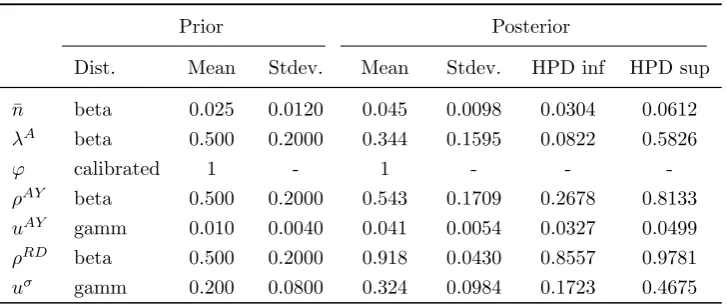
Medium-term growth prospects in the US and many developed countries have deteriorated substantially. In particular, the US Great Recession of 2008-2009 seems to have generated a persistent downward shift in the GDP trend displayed in Figure 1.
[Figure 1 about here.]
Since this has happened after the financial crisis of 2008, it suggests that the sudden unavailability of credit to investment resulting from the crisis has led to a not yet reverted GDP decline below its long-term trend. Can a temporary financial shock generate such a persistent effect? It can reduce physical capital accumulation during the crisis and the resulting credit crunch, but, according to standard macroeconomics - which assumes decreasing returns to physical capital - GDP should go back to trend after the financial trouble has ended. Alternatively, we could think of an adverse exogenous technology growth shock, perhaps occurred simultaneously with the financial crisis, or even causing it. However, the above evidence would suggest an unrealistically high persistence of such technological shock. We claim that the puzzle is solved, if we realize that technology is not ex-ogenously evolving, but is affected by research and development (R&D). And in fact, R&D investment data feature a significant temporary negative deviation of R&D investment from its trend during the financial crisis.
It is then natural to conjecture that if TFP growth results from R&D-driven innovations, the drop in the right panel of Figure 1, by implying a permanent negative deviation of productivity from its pre-crisis trend, could be at least partially explain the GDP time series.
While this channel is certainly at work, others more common in standard New Keynesian models, could be important as well: demand shocks, price and wage distortions, etc. Hence, the correct question would be: how much of the observed GDP data of Figure1is due to an R&D or physical capital investment drop, persistently insufficient private or government demand, ineffective monetary policy close to the zero lower bound (ZLB) or labor and output market distortions?
Therefore, a complete macroeconomic explanation of what has hap-pened should include R&D, innovation, and growth in addition to the standard dynamic stochastic general equilibrium (DSGE) framework. Mo-tivated by this need, we construct an integrated growth and business cycle medium scale macroeconomic model, which incorporates Schumpeterian creative destruction `a la Aghion and Howitt (1992) and Nu˜no(2011) into a New Keynesian economic framework`a la Smets and Wouters (2003) and
Kollmann et al. (2016).1 This setup allows us to estimate the model at
quarterly frequency for the US economy in a period - 1995Q1 to 2015Q1 - rich in important events involving innovation and growth - burst of the bubble, the 2009 collapse in R&D - and in business cycles and monetary policy events - financial crisis build-up and explosion, unprecedented fiscal stimulus, ZLB hit by the Fed interest rate.
Despite the importance of such an analysis, the estimated models at-tempting to do it so far are rare. Most notably Bianchi and Kung (2014) estimate a model with R&D capital exerting a positive spillover on the economy like in Frankel(1962) and Romer (1986), while Anzoategui et al.
(2016) adapt Comin and Gertler (2006) knowledge diffusion extension of Romer’s1990expanding product variety growth mechanics to show how de-mand driven slumps lead to business cycle persistence via endogenous R&D activity. Varga et al. (2016) extend this framework to a semi-endogenous growth medium scale model calibrated to US and EA data.
Guerron-Quintana and Jinnai(2015) highlight the role of financial frictions by deeply
microfounding them. Despite their insightful contributions to an emerging integrated macroeconomics2 literature, none of these papers considers
cre-ative destruction, which is the only approach consistent with the microe-conometric evidence that innovation and growth correlates positively with firm entry and firm exit.3 In fact, the variety expansion models predict
firm exit to have a negative effect on growth, which is against industry evidence suggesting that reallocation from less productive exiting firms to
1Previous successful attempts at integrating endogenous growth and business cycle
areAnnicchiarico et al.(2011),Annicchiarico and Rossi(2013), andAnnicchiarico and Pelloni(2014).
2Integrating growth and business cycle in a unified way.
3See for exampleFoster et al.(2001) influential evidence that the ongoing replacement
more productive firms is an engine of productivity growth.4
In our model, growth is endogenously driven by Schumpeterian R&D entrepreneurs’ activities and knowledge accumulation. In this formula-tion, each innovation is a new intermediate good of enhanced quality. En-trepreneurs collect funds from households to invest into R&D aimed at capturing monopoly rents. In each period they face a probability that the firm jumps to the technological frontier. If the innovation occurs, the entrepreneur earns monopoly profits until the firm is replaced by a new in-novator. On aggregate, growth of the technological frontier is the outcome of positive knowledge spillovers from R&D activities. These spillovers are subject to shocks which alter the basic research content of applied R&D. Similarly toVarga et al.(2016), our main model assumes a semi-endogenous growth structure in the innovative frontier evolution, while allowing its adoption to follow a purely endogenous growth mechanism.
On the Keynesian side, we incorporate monopolistic competition in product and labor markets as well as price and wage stickiness. Despite the importance of creative destruction, only few papers have tried to join it with price stickiness. Prominent examples areBenigno and Fornaro(2016),
Oikawa and Ueda (2015a,b,c), and Rozsypal (2016). Other standard
as-pects such as habit formation in leisure and consumption, flow adjustment costs in investment, capacity utilization, endogenous fiscal rules, and gov-ernment debt accumulation help fit observed quantity dynamics and a rich set of macroeconomic shocks is used for the estimation. In addition, the central bank follows a Taylor rule. Our analysis also considers consequences of the ZLB constraint on the policy interest rate. To guarantee realistic features also on the growth mechanism, we eliminate the strong scale effect
Jones (1995) and test our results both in a semi-endogenous and in a fully
endogenous approach.
We allow the model to nest exogenous growth as a special case, leav-ing it to the data to decide. And indeed the data confirm that frontier growth in potential GDP is driven by endogenous R&D investment. As in
Aghion and Howitt (1992) and Nu˜no(2011), innovations are the outcome
of a patent-race in every sector, with each innovation improving upon
ex-4For the importance of reallocation as an engine of growth also seeAcemoglu et al.
isting goods. Innovating firms replace the incumbent monopolist and earn higher profits until the next innovation occurs. Knowledge spillovers push the technological frontier further. Unlike existing stylized Schumpeterian growth models, the DSGE structure allows, for the first time in the endoge-nous growth literature, a sophisticated estimation of the main innovation and growth parameters. Semi-endogenous growth `a la Jones (1995), Kor-tum (1997), and Segerstrom (1998) is confirmed, but knowledge spillover coefficient confidence intervals allow a very persistent effect of shocks af-fecting R&D.
More generally, our Bayesian estimation allows us to quantify the rel-ative contribution of the various shocks in explaining the recent adverse growth experience. Investment dynamics emerges as a key driver of the Great Recession, alongside the consumer saving shock: their interaction characterizes the joint decline in physical capital, R&D investment, and consumption.5
The paper is intendedly standard, and indeed we constrain ourselves to putting together the already existing frameworks of New Keynesian and Schumpeterian growth theory. The next section are divided as follows: Section 2 describes the main model. Section 3 describes the Bayesian es-timation approach and its results, and discusses numerical simulations. Section 4 shows the robustness of our main model results under impor-tant alternatives: a scale-free fully endogenous growth framework, and two hybrid versions which allow some degree of exogenous growth in either semi-endogenous and fully endogenous frameworks. Section 5 concludes.
2
Model
This section lays out the economic environment. Being ours a fairly rich medium-scale macroeconomic model, we will here provide only the main aspects of its components: households, manufacturing production, inno-vation, monetary and fiscal authorities, market clearing conditions, and
5Anzoategui et al.(2016) use a “liquidity” shock to generate the positive co-movement
exogenous structural shocks.6 To keep exposition lean, we relegate the
most cumbersome details to Appendix B.
2.1
Households
There is a continuum of households indexed by j ∈[0,1]. Households are split in two groups: Savers (“Ricardians”, superscripts) who own the firms and hold government bonds, and constrained households (“rule-of-thumb” consumers, superscript c) whose only income is labor income and who do not save nor borrow. The share of savers in the population is ωs. The
lifetime utility of a household of either type r=s, cis defined as
Ur jt =
∞
X
q=t
exp(ǫC t)β
q−t
us(·), (1)
whereβ denotes the discount factor, andǫC
t is an exogenous savings shock
distorting the household’s discount factor. Both types of households en-joy utility from consumption Cr
jt and incur disutility from labor Njtr.7 In
addition, the utility of Ricardian households depends on financial assets held.
2.1.1 Ricardian Households
Ricardians work, consume, own all firms, purchase risk-free bonds as well as government bonds and receive nominal transfersTs
jt from the government.
They have access to financial markets and hold financial assetsF Ajt. Total
financial wealth consists of government bonds Bjtg, private risk-free bonds
Bjtrf, and shares PS
t Sjt. PtS is the nominal price of shares in t and Sjt the
number of shares held by household j:
F Ajt =Bjtg +B rf
jt +P
S
t Sjt. (2)
6The present model shares standard features withKollmann et al. (2016), with the
major distinction of introducing endogenous innovation in place of fully exogenous tech-nological progress.
7At any given moment of time Nr
t households of type r work. We assume perfect
We define the gross nominal return of an asset St as ist. Therefore, the
budget constraint of a saver household j can be written as:
Pt(1 +τc)Cjts +F Ajt = 1−τN
WtNjts + P S
t +Ptdt
Sjt−1 + (1 +i g t−1)B
g jt
+ (1 +irft−1)B rf
jt +T
s
jt+ Πt−taxsjtexp(ǫ T AX
), (3)
where Pt denotes the GDP deflator and τc is a consumption (VAT) tax.
τN is the tax rate levied on wages W
t, dt are dividends from intermediate
good producers, igt−1 is the interest rate of governmental bonds and i rf t−1
is the risk-free rate. Ts
jt are government transfers to savers. Πt denotes
the profits all the firms other than intermediate goods producers. taxs jt are
lump-sum taxes paid by savers subject to a tax shock ǫT AX.
Each Ricardian household j maximizes its lifetime utility:
us Cs jt, Njts,
UA jt−1
Pt
!
= 1 1−θ C
s
jt−hCts−1
1−θ
− ω
nexp(ǫU t )
1 +θN (C s t)
1−θ
Ns jt−h
NNs t−1
1+θN
+ Cs
jt−hC
s t−1
−θ U A jt−1
Pt
, (4)
with Cs
t =
Rωs
0 C
s
jtdj. h and hN ∈ (0,1) measure the strength of external
habits in consumption and labor, and ωn is the relative weight of labor
in the utility function. ǫU
t is a labor preference shock common in the real
business cycle literature. To allow for realistic spreads, we microfound the risk premium shock as in Kollmann et al. (2016) by assuming that savers’ preferences for real financial wealth, (F Ajt)/(Pt), may fluctuate as well
according to
UjtA−1 = exp(ǫ B
t) α
B0
Bjt−1
+ exp(ǫSt) α S0
Pts−1 Sjt−1
, (5)
where ǫB
t and ǫSt represent time varying risk premium shocks on bond and
different marginal utilities for different assets captured by αB0 and αS0.8
2.1.2 Constrained households
Constrained households do not participate in financial markets. In every period they consume all their disposable income from wages and govern-ment transfers. This results in the following period-by-period budget con-straint:
Pt(1 +τc)Cjtc = 1−τ
N
WtNtc +T c
t −tax
c jtexp(ǫ
T AX
), (6)
where taxc
jt are lump-sum taxes paid by constrained households. The
in-stantaneous utility function for a liquidity constraint households is
uc Cjtc, N c jt
=exp(ǫ
C t )
1−θ C
c
jt−hC
c t−1
1−θ
−ω
nexp(ǫU t )
1 +θN (C c t)
1−θ
Nc jt−h
NNc t−1
1+θN
, (7)
where Cc
t =
R1
ωsC
c jtdj.
2.2
Intermediate Goods
Eachithdifferentiated intermediate good is produced by a monopolistically
competitive firm using total capital Ktot
it−1 and labor Nit. The production
function is Cobb-Douglas:
Yit=AYit(Nit)a
cuit
Ktot it−1
AY t
1−a
, (8)
where a denotes the labor share, AY
it is a sector specific productivity level
andcuit is firm-specific level of capital utilization. With more sophisticated
technologies, production becomes more capital-intensive. AY
t =
R1 0 A
Y itd i
is the average productivity across all sector in the differentiated goods production. The average output across sectors is Yt=
R1 0 Yitd i.
8Our steady state restrictions imply that αB0 is positive while αS0 is negative. In
As a consequence of (8) sectors with higher relative technological sophis-tication benefit more from the average technological level across sectors:9
Yit =
AY it
AY t
| {z } rel. technology level
AY t Nit
a
cuitKittot−1
1−a
. (9)
Total Factor Productivity, T F Pt, is therefore:
T F Pt= AYt
a
. (10)
Firm i’s capital stock evolves as
Kit= (1−δ)Kit−1+Iit, (11)
where δ is the capital depreciation rate, and Iit denotes gross investment
in physical capital. Public capital Kitg follows an analogous law of motion.
Total capital is the sum of both
Kittot =Kit+Kitg, (12)
assumed, for the sake of simplicity, to be perfect substitutes.
Intermediate good firms choose prices, employment, and capacity uti-lization as well as capital and investment to maximize dividends subject to the production technology (9) and the physical capital law of motion (11). Dividends are given by
dit= 1−τK
Yit−
Wt
Pt
Nit
+τKδKit−1−Iit−adjit, (13)
where τK is a corporate income tax, adj
it are total adjustment costs
as-sociated with price and labor adjustment or changing capacity utilization, and investment. The firm problem is standard and details are referred to AppendixB.1.
9This formulation allows us to avoid keeping track a of a distribution of firms and
2.3
Final Good Producers and Labor Markets
The remaining sectors of manufacturing production are kept intendedly standard. Therefore, we only summarize key elements and refer details to Appendix B.2-B.3. Perfectly competitive firms produce a final good Yt
using differentiated intermediate inputs. Wages in the intermediate good production are set by a monopolistically competitive trade union at a mark-up, µw
t. To capture rich labor market dynamics, we allow for real wage
rigidities (see Blanchard and Gal´ı 2007), governed by parameter γwr.
2.4
Endogenous Innovation
We start with the detailed description of the endogenous technological progress structure of our model.
Innovations. Innovations generate growth. In each period t the pro-ductivity of a sector AY
it jumps to the technology frontier A Y,max
t with
probability nit−1. The frontier is publicly available and represents the
most advanced technological level across all sectors defined as AY,t max ≡
max{AY
it|i∈[0,1]}. Productivity in each sector i evolves as:
AY it =
(
AY,t max, with probability nit−1
AY
it−1, with probability 1−nit−1
)
. (14)
Entrepreneurs. Innovations are the result of entrepreneurial investments into R&D. The probability of reaching the frontier is itself endogenous. In each sectoriin each periodtan entrepreneur is randomly selected with the opportunity to try to innovate.10 If such entrepreneur’s R&D firm invests
R&D costXRD
it it will produce a probability nit of a successful innovation,
which entails the discovery of a new intermediate good with next period’s frontier productivityAY,t max. We assume that research will be more difficult
if the overall technology frontier is more advanced, i.e. per unit research costs increase with the frontier productivity AY,t max. The probability of
innovation in the sector, assumed independent across sectors, has the
fol-10Hence, innovative ideas are scarce as they “arrive to random agents at random
lowing production function:
nit =
XRD it
λRDAY,max it+1
1 (η+1)
, if XRD
it < λRDA Y,max
t+1
1, if XRD
it ≥λRDA
Y,max
t+1
, (15)
where λRD > 0 is an R&D difficulty parameter and η > 0 accounts for
decreasing returns of R&D. In our discrete time setting, we will assume that an innovation occurring at time t will permit production in period
t+ 1. Moreover, the second line of (15) is needed to guarantee that the probability of innovation per period11 is no larger than 1.
By Bertrand competition, the patent holder of the new good will pro-duce by definition the good of highest quality and, following a price war, will replace the existing incumbent monopolist and appropriate all the sec-torial profits from t+ 1 on. Hence, it is the prospects of becoming next period’s incumbent manufacturing monopolist in the sector that creates the incentives to invest in R&D at time t. Since the new entrant does not in-ternalize the loss incurred by the previous incumbent, creative destruction may imply too much or too little R&D investment.12
For symmetry with the other parts of the model estimation, which in-clude adjustment costs, we will assume the existence of adjustment costs in the R&D as well. The R&D adjustment cost function13 is defined as
adjRD it (X
RD
it )≡
γRD
2Yt
(XRD
it −X
RD t−1gY)
2, (16)
where gY denotes output trend which makes adjustment costs stationary.
Innovation at time t is like a static lottery, and given individual risk aversion, we assume that the R&D firm in each sector finances the risky innovation from a fund set up by Ricardian households to completely di-versify, by the law of large numbers, innovation risk across the continuum
11Which instead in a continuous time framework could be any non-negative number.
12A horizontal innovation framework, by missing this business stealing externality,
would imply too little R&D in equilibrium.
13The interpretation of adjustment costs in a creative destruction environment
of sectors, with uncorrelated risk, in the economy. To capture realistic fluc-tuations of R&D investment, we allow for a stochastic R&D-specific invest-ment risk premium required by the fund, ǫAY
t . The R&D entrepreneurial
problem is then a simple expected profit maximization:
max
XRD it
=nit
PSdmax
it
Pt
−XRD
it +adj
RD it (X
RD it )
1 +ǫAY t
, (17)
where PSdmax
t is the nominal stock market value of the firm at the
techno-logical frontier.
The value of becoming the incumbent is the same across sectors and hence, in equilibrium, the R&D investment cost is symmetric,XRD
it =XtRD,
as is the probability of success nit = nt. The R&D optimality condition,
after making use of (15), then becomes:
nt
(η+ 1)
PSdmax
t
Pt
=XtRD
γRD
Yt
(XitRD −X RD t−1gY)
(1 +ǫAYt ). (18)
Note that R&D firms earn positive profits as long η >0.14
Finally, by the law of large numbers,ntalso measures the fraction of the
total number of sectors which innovate each period, as well as the fraction of firms that exit and enter the market. The higher the equilibrium value of
nt the stronger innovation and creative destruction, and the more dynamic
the set of innovative industries.
Stock Market Value. Differentiated goods producing firms are owned by households. The value of these firms at timet isPS
t Sttot =PtS where we
normalize the total number of stocks Stot
t to 1. In our economy firms are
heterogeneous and firm turnover follows innovation. Hence, due to Schum-peterian creative destruction, a fractionnt−1 of obsolete firms belonging to
time t−1 portfolio is lost at time t, replaced by new entrants with higher stock market value PSmax
t . Taking that into account, the gross nominal
14As long as the equilibrium probability is less than 1, we could easily consider the
return on the aggregate time t stock market portfolio is given by:
1 +is
t =
Et
dt+1Pt+1+PtS+1−ntPtS+1max
PS t
. (19)
We include in the return on period t equities the value of the average dividend paymentsdt+1, we also take into accounts capital gains and losses.
The average timet+1 portfolio,PS
t+1, also includes the innovative firms that
have replaced fraction nt of time t industry. Hence, we have to subtract
their aggregate value,ntPtS+1max, from it. This reasoning is reflected in (19).
Frontier Value. Frontier technology index net growth rate gAY,max
t is
defined as
gAY,max
t =
AY,t max−A Y,max
t−1
AY,t−max1
. (20)
Entrepreneurs collect funds from households. They invest into R&D to reach the technological frontier, patent its adaptation to their sector, and appropriate the resulting production monopoly. Hence, each entrepreneur at the frontier earns the monopoly profits resulting from the highest quality intermediate good: these profits, and the resulting dividends, are (AY,t max)/(AYt )
times bigger than those of the average technology firm. Therefore, the nominal stock market value as of time t, PSmax
t , of a firm that will start
producing at the technology frontier at timet+ 1 must obey the following expression:
PSmax
t =
Et
Pt+1dt+1
AY,t+1max AY
t+1
+ PtS+1max
g
AY,t+1max
(1−nt+1)
(1 +is t)
. (21)
Notice that since patents of the latest and most advanced technological require one period of implementation, for an innovation developed in period
t, production and dividend flows only start in t + 1. Furthermore, the continuation value in the stock market in t+ 1 takes into account that competitors may successfully innovate, with probability nt+1, and render
it unusable in period t+ 2. In case no innovation is found in the sector in period t+ 1, which happens with probability 1−nt+1, the firm’s value
than that of a generic newly entered innovator by a factor equal togAY,max
t+1 .
This explains the last part of the numerator of eq. (21).
Frontier and diffusion. The growth of technological frontier,gAY,max
t , is
the outcome of positive knowledge spillovers from the aggregate innovation efforts as in Howitt and Aghion (1998). According to this Schumpete-rian view, R&D activities have an appropriable applied content, i.e. the patentable sectorial adoption of the technological frontier, and an unappro-priable basic aspect, which pushes the aggregate frontier further. The basic content of aggregate R&D freely spills over to all sectors. The way in which this R&D spillover operates is not deterministic, but as in Nu˜no(2011) it is affected by time-varying spillovers σRD
t . This captures the potentially
volatile basic research content of applied R&D, which could reflect, in re-duced form, the scientists and engineers orientation, the university policies, and variable regulatory aspects of intellectual property rights (IPRs). More in detail, we assume that
AY,t max =A Y,max
t−1 +
AY,t−max1
ϕXRD t−1
Yt−1
Nt−1
λA
σRD
t , (22)
where ϕ < 1 reflects decreasing returns to the intertemporal knowledge spillover as in Jones (1995), while 0 < λA <1 is a standard “stepping on
toes” R&D congestion externality parameter capturing research duplica-tion, knowledge theft, etc. Jones and Williams (2000). This idea was also used in the medium scale policy focused macroeconomic models of Roeger
et al. (2008) and Varga et al.(2016).
The instantaneous knowledge spillovers follows an exogenous process given by
σtRD =σ RD
exp(ǫσt), (23)
whereǫσ
t is an R&D spillover shock andσRD are steady state spillovers. Eq.
(22) says that the technological frontier increases in its previous period’s value, and also in the fraction of the employees indirectly working in R&D (given by XtRD−1
rate of the technological frontier as:
gAY,max
t =
X
t−1
Yt−1Nt−1 λA
σRD t
AY,t−max1
1−ϕ . (24)
Log-differencing the previous equation, it follows that in a balanced growth path (BGP) - in which gAY,max
t and
Xt−1
Yt−1 are constant - the following holds:
gAY,max
t =
λAg P OP
1−ϕ . (25)
As in Jones (1995) the growth rate of the frontier, in the long-run, is gov-erned by the growth rate of populationgP OP. The factor of proportionality
depends on the extent of decreasing returns, inversely represented by λA.
It is important to notice that unlike Jones (1995) and Varga et al. (2016) our growth ofAY,t maxdoes not refer to the growth rate of patents but rather
to the growth rate of frontier productivity index. While this is obviously derived from the flow of new patents invented, its numerical value is al-ready filtered by effect of patents on productivity. Therefore, we should expect a much lower value of λA than in Jones and Williams (2000) and
Varga et al. (2016).
Unlike Nu˜no(2011) and similarly to Varga et al. (2016), the evolution of the technological frontier in our model is semi-endogenous, as in Jones
(1995) while its adoption remains fully endogenous, as inComin and Gertler
(2006) and Anzoategui et al. (2016). This formulation not only permits to eliminate the counterfactual strong scale effects that plagued the early generation endogenous growth models, but also avoids steady state growth effects of policy variables and shocks, which facilitates the comparison with the standard exogenous growth DSGE models.
aggregation: AY t = Z 1 0 n
nit−1A Y,max
t + (1−nit−1)A
Y it−1
o
d i
=nt−1
AY,t max−A Y t−1
+AYt−1, (26)
where we have also used our previous symmetry result, nit−1 =nt−1. On a
balanced growth path the frontierAY,t maxgrows at the same rate as average
technological level defined in (26).
2.5
Monetary and Fiscal Authorities
The nominal policy interest rateitis set by the monetary authority
accord-ing to a Taylor rule:
it−¯i=ρi(it−1−¯i) + 1−ρ i
ηiπ(πt−π¯) +ηiyy˜t
+ǫit, (27)
where ¯i=r+ ¯π is the steady state nominal interest rate, equal to the sum of the steady state real interest rate and steady state inflation. ˜yt is the
output gap15 and ηiπ>1 and ηiy >0. ǫi
t is a white noise shock.
Government consumption and physical capital investment are set ac-cording to the following fiscal policy rules:
cGt −c G
=ρG(cGt−1−c G
) +ǫGt (28)
iG
t −iG =ρIG(iGt−1−i
G) +ǫIG
t , (29)
where cG
t ≡
Gt
Yt and i
G
t ≡
IG t
Yt are government consumption and investment
as a share of GDP.16ǫG
t and ǫIGt are white noise disturbances. Government
transfers to households follow this policy rule:
τt−τ =ρτ(τt−1−τ) +η def
Btg−B g t−1
Yt
−def
+ηB
Btg
Yt
−b
+ǫτ t, (30)
where τt ≡ TYtt are net nominal transfers normalized by GDP. Btg denotes
total nominal government debt owned by households, ηdef is a deficit
coef-15Output gap is measured by ˜y
t=log(Yt)−ytwhereytis (log) output trend.
ficient, ηB is a debt coefficient. ǫT
t is a white noise transfer shock.
Govern-ment debt and transfers react to their associated GDP-adjusted targets,
def and b. The government budget constraint, is
Btg = 1 +i g t−1
Btg−1−R G
t +PtGt+PtItG+Tt, (31)
where 1 +igt denotes the interest rate on government debt and RGt is the
nominal revenue of the government.
2.6
Resource constraint
Market clearing requires
Ct =ωsCts+ (1−ω s
)Ctc (32)
and, additionally, Ns
t =Ntc = Nt and Tts =Ttc =Tt. Labor markets clear
and financial assets clearing requires St = 1 and Bt = Btg. Finally, the
aggregate budget identity takes R&D investment into account
Yt=Ct+It+Gt+ItG+adjt+XtRD. (33)
2.7
Exogenous processes
All exogenous shock processes of type x (unless specified explicitly) follow autoregressive processes of order one with an autocorrelation coefficient
|ρx|<1 and innovationux
t. Thus,
ǫt=ρxǫt−1+u x
t. (34)
3
Results
3.1
Data and Estimation Approach
remain-ing parameters with Bayesian methods.17 In particular, we apply the Slice
sampling algorithm (Neal 2003 and Planas et al. 2015) because of its im-proved efficiency and accuracy.18 In total we use data on 21 macroeconomic
time series ranging from 1995Q1 until 2015Q1. Data are taken from the Bureau of Economic Analysis (BEA) and the Federal Reserve. Appendix
A provides additional details.
It is worth noticing that in the estimation procedure, we have a number of parameters calibrated by directly using the steady state restrictions and others which are obtained by Bayesian estimation. The two procedures are interdependent, because the estimated parameters also affect the calibrated parameters, which are usually functions of them, and vice versa. We here mention an important example of this interdependence, in which the steady state restriction equation (25) is used to determine λA as a function of the
estimated parameters. In fact, since
T F Pt= AYt
a
, (35)
it follows that in steady state the observable growth rate of TFP isgT F P =
agAY =agAY,max. This equation in turn implies that we can use the steady
state growth rate relationship to calculate parameterλAas soon as we have
an estimated parameter ˆϕ and a. In fact, based on the previous equations we can write:
λA= (1−ϕˆ)−1 gT F P
agP OP
. (36)
3.2
Calibrated parameters
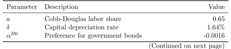
[image:19.595.111.484.619.698.2]Table 1 reports values for calibrated parameters.
Table 1: Calibrated Parameters
Parameter Description Value
a Cobb-Douglas labor share 0.65
δ Capital depreciation rate 1.64%
αB0 Preference for government bonds -0.0016
(Continued on next page)
17We implement the solution and estimation in Dynare (Adjemian et al. 2011).
18Our findings are robust to other sampling algorithms, such as general
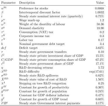
Table 1: (continued)
Parameter Description Value
αS0 Preference for stocks 0.0068
β Intertemporal discount factor 1.0032 ¯i Steady state nominal interest rate (quarterly) 0.75%
µw Wage mark-up 1.2
ωN Weight of the disutility of labour 58.36
σy Demand elasticity 18.90
τc Consumption (VAT) tax 0.2
τK Corporate income tax 0.3
τN Labor tax 0.17
b Nominal government debt target 3.4
def Deficit target 3.62%
τ Steady state government transfers 0.10
iG Steady state private investment share of GDP 15.5%
C/GDP Steady state private consumption share of GDP 67.2%
cG Steady state government share of GDP 17.1%
η R&D decreasing returns 5.72
λRD R&D difficulty exp(17.61)
σRD Steady state R&D spillovers 0.82%
¯
XRD Steady state value of cost of R&D 1.56% λA Stepping on toes R&D congestion 0.25
¯
gAY Constant for growth of productivity 0.36% ¯
gP OP Constant for growth of population 0.24%
¯
π Constant for GDP deflator inflation 0.47% ¯
gY Constant for growth of GDP trend 0.60%
¯igBg Steady state Government interest payments 3.17%
The labor share in the production function,a, is set to 0.65. The capital depreciation rate, δ, is implied by the empirical averages of private capital and investment and equal to 1.64 percent quarterly. The discount rate, β, implies a steady state value of the stochastic discount factor of 0.99. This restriction allows to derive a value for the preference of households on hold-ing stocks, αS0, from their optimal shares choice. The steady state wage
mark-up, µw, is set to 1.2, whileωN is endogenized from the labor supply
equation conditioning on the observed empirical average of the wage share. Normalizing steady state employment to unity, allows to derive the steady state price mark-up from the labor demand equation. Given the markup, the pricing equation is used to determine the value of the demand elasticity,
[image:20.595.117.488.133.494.2]to 0.2 and 0.3, while the labor tax is endogenized from the government revenue. The targets for total nominal government debt and deficit as well as public investment and consumption and government transfers, are set equal to the respective empirical averages. The empirical average of the interest payments on government bond (¯igBg around 3 percent) allows to
place a restriction on the parameter αB0. Steady state ratios of the
pri-vate consumption and investment share of GDP match empirical averages. In the R&D block, we impose the empirical average of the share of R&D investment over GDP and the estimated mean value of the probability of reaching the frontier technology, ¯n, to derive the implied value of the R&D difficulty,λRD and the parameterηfrom the definition of production
function of nt (15) and the optimality condition of innovators (18). The
mean value of the R&D spillovers comes from the semi-endogenous frontier definition (22) given the empirical value of the technology growth rate.
3.3
Estimated parameters
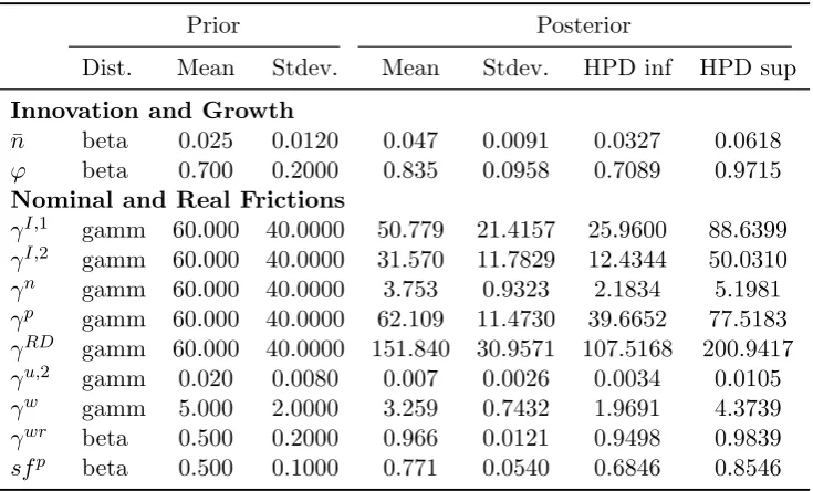
[image:21.595.115.483.501.723.2]This section provides the estimates of the main model described in the previous sections. The main results of our most refined estimation can be seen in Table 2.
Table 2: Priors and Posteriors of Estimated Parameters
Prior Posterior
Dist. Mean Stdev. Mean Stdev. HPD inf HPD sup
Innovation and Growth
¯
n beta 0.025 0.0120 0.047 0.0091 0.0327 0.0618
ϕ beta 0.700 0.2000 0.835 0.0958 0.7089 0.9715
Nominal and Real Frictions
γI,1 gamm 60.000 40.0000 50.779 21.4157 25.9600 88.6399
γI,2 gamm 60.000 40.0000 31.570 11.7829 12.4344 50.0310
γn gamm 60.000 40.0000 3.753 0.9323 2.1834 5.1981 γp gamm 60.000 40.0000 62.109 11.4730 39.6652 77.5183
γRD gamm 60.000 40.0000 151.840 30.9571 107.5168 200.9417 γu,2 gamm 0.020 0.0080 0.007 0.0026 0.0034 0.0105
Table 2: (continued)
Prior Posterior
Dist. Mean Stdev. Mean Stdev. HPD inf HPD sup
sfw beta 0.500 0.1000 0.519 0.0998 0.3378 0.6593
Fiscal Policy
ηB beta 0.010 0.0050 0.000 0.0001 0.0000 0.0003 ηdef beta 0.030 0.0080 0.013 0.0018 0.0106 0.0159
Monetary Policy
ηi,π beta 2.000 0.4000 1.970 0.3658 1.3740 2.5851 ηi,y beta 0.250 0.1000 0.149 0.0379 0.0894 0.2001
Preferences and Households
h beta 0.500 0.2000 0.839 0.0331 0.7880 0.8924
hN beta 0.500 0.2000 0.631 0.2051 0.3309 0.9339
θN gamm 2.500 0.5000 2.114 0.3850 1.5203 2.7155 θ gamm 1.500 0.2000 1.404 0.1603 1.1482 1.6191
ωs beta 0.650 0.0500 0.763 0.0151 0.7394 0.7860
[image:22.595.116.483.133.352.2]This table reports values estimated parameters of the baseline model. HPD inf and HPD sup refer to the 90 percent highest posterior density interval.
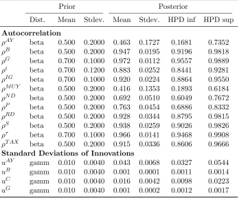
Table 3: Priors and Posteriors of Shock Processes
Prior Posterior
Dist. Mean Stdev. Mean Stdev. HPD inf HPD sup
Autocorrelation
ρAY beta 0.500 0.2000 0.463 0.1727 0.1681 0.7352 ρB beta 0.500 0.2000 0.947 0.0195 0.9196 0.9818 ρG beta 0.700 0.1000 0.972 0.0112 0.9557 0.9889
ρi beta 0.700 0.1200 0.883 0.0252 0.8441 0.9281 ρIG beta 0.700 0.1000 0.920 0.0224 0.8864 0.9550
ρM U Y beta 0.500 0.2000 0.416 0.1353 0.1893 0.6184
ρN D beta 0.500 0.2000 0.692 0.0510 0.6049 0.7672 ρP beta 0.500 0.2000 0.763 0.0454 0.6886 0.8332 ρRD beta 0.500 0.2000 0.928 0.0344 0.8795 0.9815
ρS beta 0.500 0.2000 0.938 0.0259 0.9026 0.9826 ρτ beta 0.700 0.1000 0.966 0.0141 0.9468 0.9908 ρT AX beta 0.500 0.2000 0.915 0.0336 0.8606 0.9666
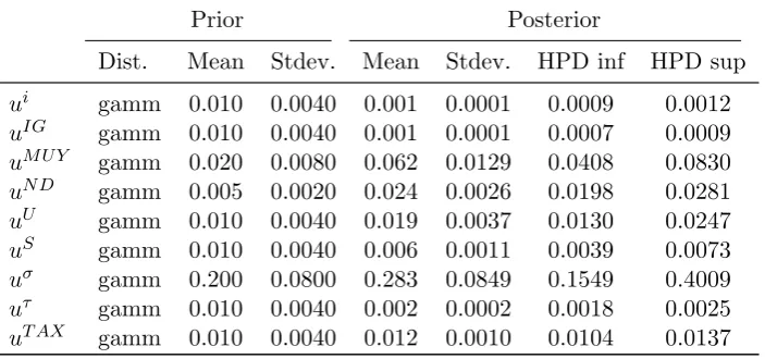
Standard Deviations of Innovations
uAY gamm 0.010 0.0040 0.043 0.0068 0.0327 0.0544 uB gamm 0.010 0.0040 0.001 0.0001 0.0011 0.0014
[image:22.595.126.475.446.734.2]Table 3: (continued)
Prior Posterior
Dist. Mean Stdev. Mean Stdev. HPD inf HPD sup
ui gamm 0.010 0.0040 0.001 0.0001 0.0009 0.0012 uIG gamm 0.010 0.0040 0.001 0.0001 0.0007 0.0009
uM U Y gamm 0.020 0.0080 0.062 0.0129 0.0408 0.0830
uN D gamm 0.005 0.0020 0.024 0.0026 0.0198 0.0281 uU gamm 0.010 0.0040 0.019 0.0037 0.0130 0.0247
uS gamm 0.010 0.0040 0.006 0.0011 0.0039 0.0073 uσ gamm 0.200 0.0800 0.283 0.0849 0.1549 0.4009 uτ gamm 0.010 0.0040 0.002 0.0002 0.0018 0.0025 uT AX gamm 0.010 0.0040 0.012 0.0010 0.0104 0.0137
This table reports values of autocorrelations and standard deviations of all shock processes. HPD inf and HPD sup refer to the 90 percent highest posterior density interval.
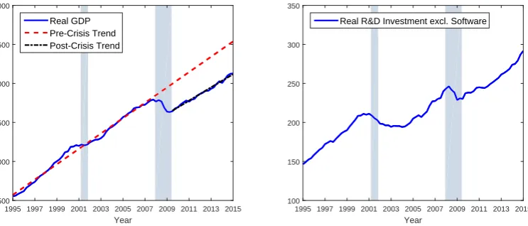
We report the assumed prior distribution of each parameter as well as its prior mean and standard deviation, and the posterior distribution obtained with our Bayesian estimation procedure, including its mean, standard de-viation, and 90 percent confidence interval lower and upper bounds.
As we can see from Table 2, thanks to our extremely rich macroeco-nomic model we have been able to estimate some important parameters for semi-endogenous growth, which the literature on economic growth could never satisfactorily estimate so far, but rather relied on simple calibration procedures. Most notable is the knowledge stock intertemporal spillover parameter ˆϕ, which has an estimated mean equal to 0.835. This param-eter estimate is significantly below 1 even though, in particular, we have included a non-zero prior density inϕ = 1. Hence, the estimation supports semi-endogenous growth in the US macroeconomy.
[image:23.595.124.476.133.298.2]model. The lower bound of the 90 percent confidence interval (0.7089) is still close enough to 1 to guarantee a relatively long transition to the semi-endogenous balanced growth path, while its upper bound, 0.9715, is extremely close to 1, and hence suggesting that this model could have policy predictions practically indistinguishable from those of a fully endogenous growth model.
Quite striking is also the estimate of the R&D adjustment costs pa-rameter, γRD , whose estimated posterior mean, 151.84, is the highest
adjustment cost parameter of the whole model. This result is important because it suggests that the R&D and growth models in the academic lit-erature so far, by ignoring R&D adjustment costs, may lead to potentially misleading predictions on the effect of policies on growth. So high R&D adjustment costs indicate that the R&D response to policies could be much more sluggish than usually thought.
Moreover, exogenous R&D spillover shocks in this model seem to be very persistent. The autocorrelation coefficient of the R&D spillover shock
ǫσ
t, which appears in Table 3 as ρRD, has a 90 percent confidence interval
ranging from 0.8795 to 0.9815. This estimate has policy implications too. As long as the R&D spillover shock is influenced by IPRs policy, a policy or jurisprudence shift of researcher’s incentives towards more narrow focus on the adaptation of the frontier to marketable products, rather than on more basic research discovery, may have long lasting negative effects on frontier productivity growth. This persistence could also be due to the common law structure of the United States legislative process, which implies that a civil law policy change could fully disclose it potential for the economy only after a long enough series of court precedents have been ruled, as predicted
byCozzi and Galli (2014). The next section will highlight the dynamics of
the estimated shocks by studying the impulse response functions (IRFs) of our main model.
3.4
Model Dynamics
the economy. All shocks are assumed temporary, i.e. lasting only one term. An important shock in this model is the shock on the R&D risk pre-mium requested by investors to finance R&D firms. Figures 2displays the corresponding IRFs.
[Figure 2 about here.]
[Figure 3 about here.]
As predicted based on the posterior estimates of Table 2, despite the absence of permanent growth effects of temporary shocks due to the semi-endogenous nature of R&D-driven growth of this model, a temporary (one quarter) R&D investment risk premium shock could have implications last-ing several years. Since the quarter (i.e. three months) is our assumed time unit, we can see that the average technology and GDP effects of a tempo-rary R&D investment shock will be getting stronger and stronger even 40 quarters (that is 10 years) after its initial impulse. This long-lasting effect advises financial authorities to put effort into guaranteeing that innovators are not declined funding at reasonable conditions.
It is also interesting to see, in Figure3, the IRFs following a temporary shock to R&D spillovers. The effect of a one quarter shock to the R&D spillover on GDP and productivity can be long lasting. This persistence advices the IPR and research policy institutions to be careful in guarantee-ing that the R&D focus of researchers remains broad and supportguarantee-ing for an open science environment: this will benefit frontier knowledge expansion and will allow overall TFP and GDP to prosper.
savings that would otherwise go to a different form of investment, while the indirect effects are likely negative due to reduced market size generated by the drop in investment demand and ensuing multiplier effects.
[Figure 4 about here.]
[Figure 5 about here.]
As suggested from Figure4, an increase in the investment risk premium will reduce GDP, but will have an ambiguous and non-monotonic effect on the R&D investment, due to the complex general equilibrium dynamics involved, including the above mentioned direct and indirect effects. While, as would be normal in a model without endogenous productivity, there is a negative medium term impact on GDP, the presence of R&D in the model allows to identify a partially offsetting effect of the earlier recovery of R&D investment and ensuing recovery of technological and total factor productivity growth.
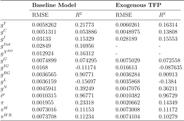
It is useful to contrast the IRFs to a model without semi-endogenous growth (i.e., an exogenous TFP model). Also in this exogenous TFP model, we allow for stochastic components of productivity growth. However, in-stead of being determined endogenously via a Schumpeterian growth mech-anism, productivity follows an exogenous (stochastic) law of motion:
AY
t =gAY,t+ǫT AY,t (37)
wheregAY,t=ρGAYgAY,t−1+(1−ρGAY)gAY+ǫLAY,tis a stochastic
productiv-ity trend. ǫT AY,tandǫLAY,t are exogenous shocks as in eq. (34). This model
abstracts from innovation, i.e. the probability to innovate is nt= 0∀t. To
facilitate comparison, all shocks are normalized to one percent standard deviation.
In the IRF graphs we have seen so far, we have used the estimated parameters and therefore policy and transition functions to simulate the effect of each structural shock in isolation. This procedure is interesting to better identify the associated macroeconomic channels and to suggest policy implications, but of course it is still a theoretical exercise under ideal controlled conditions. In the real observed data we never see only one shock operating and only one impulse of it: all shocks are active in changing sizes and directions and in every period. Therefore, the resulting macroeconomic dynamics of our DSGE model is much more complex than we could see from the above impulse response graphs. It is this complexity that permits to replicate the complex features of the observed data, and we will exploit it in the next section.
3.5
Historical Decomposition
We proceed to quantify the relative contribution of exogenous shocks in explaining the data through the lens of our estimated fully-fledged DSGE model with Schumpeterian growth. Figure 6presents a historical variance decomposition of the observed time series of real GDP growth. Each panel shows the contribution of an innovation. The continuous line displays the observed demeaned time series. Stacked vertical bars indicate the estimated relative contribution of this shock.
[Figure 6 about here.]
Several important features of the US economy in the 1995Q1-2015Q1 pe-riod emerge from our estimated shock decomposition. In particular, the most important negative contribution during the Great Recession of 2008-2009 came from the overall investment risk shock (pink) and the private saving shock (black). Their joint occurrence reflected a sudden and strong deterioration of the financial sector: the credit channels from the household savings to the private firms investing in physical capital and R&D became less reliable, and the production and the R&D sectors could not get funding comparable to the pre-crisis trend.
a result of the simultaneous drops in consumption and investment aggre-gate private demand fell, negatively affecting GDP growth. While at first monetary policy turned to an expansionary stance, reflected by the positive contribution of the green shock, when it hit the ZLB it became unable to bring the policy interest rates into the negative territory, as would have been dictated by the pre-crisis Taylor rule, and it became unable to give enough relief to the financially strained firms and households. The Fed was necessarily forced to run a more restrictive monetary policy than dictated by the Taylor rule, which is reflected by the negative contribution of the monetary policy shock to GDP growth. Other aspects of the Fed’s policy, however, seem to have succeeded in repairing the post-crisis financial sec-tor, and in fact we see it reflected by the end of the negative contribution of the investment and saving risk premium shocks starting in 2010.
The blue bars dynamics suggest that fiscal policy must have helped the US economy only upon impact, but its overly-expansionary character, by increasing public debt accumulation nearly out of control (even eventually hitting the government shutdown bound) was not able to give a persistently positive contribution to GDP growth: its cumulative contribution became negative in the second part of 2009.19
Following the crisis, firms seem to have been subject to a more com-petitive environment, as shown by the positive GDP growth effects of the negative price mark-up shocks (light red bars). Instead, the labor market seems to have suffered rigidities in the two years after the crisis, represented by harmful wage mark-up shocks - shown in yellow in the figure.
Interesting is also the picture emerging from the shock decomposition around the 2001 dotcom bubble burst. The adverse financial conditions associated with the potentially persistent harmful investment and saving shocks in the figures were at least partially offset by a strongly expansionary monetary policy stance, also corroborated by expansionary fiscal policy.
Our estimated macroeconomic model allows to identify interesting as-pects of the R&D and innovation sector. In fact, we observe a persistently negative contribution of the R&D spillover shock (brown bar) starting in
19This observation may also reflect the expectation of higher future taxes associated
2002. This observation is a startling confirmation of the negative effects of too strict IPRs which penalized academic and basic research in the US innovation system following the Madey vs Duke Supreme Court verdict of 2002, which formally ended the so called “research exemption” doctrine, which previously permitted patented discoveries to be freely used for re-search purposes without incurring the risk of patent infringement (seeCozzi
and Galli 2014).
[Figure 7 about here.]
How does the model interpret the time series on R&D investment? Figure 7 presents a variance decomposition of R&D investment. Our es-timation explains the drop in R&D investment mainly by a rise in R&D risk premia and, during periods of financial distress, also in investment risk premia. The malfunctioning of financial markets has a strong adverse effect on R&D investment. The constrained ability of financial markets to channel savings thus helps explain the low growth following the Great Recession. The slow recovery from severe financial crises has also been emphasized by recent literature (e.g.,Boissay et al. 2016). Apart from the dot-com bubble and the short pre-crisis boom, R&D spillovers affect R&D investment mostly negative. Moreover, wage mark-up and monetary policy shocks contribute to fluctuations in R&D investment.
3.6
Shocks at the Zero Lower Bound
Following the Great Recession, at least through late 2015, the ZLB on interest rates was effectively binding and hampered the Fed’s ability to stimulate the economy by further lowering the policy rate. Formally, we impose the ZLB constraint on the net nominal interest rate by modifying the Taylor rule in equation (27) to:
it =
(
ρii
t−1+ (1−ρ
i) (−¯i+ηiπ(π
t−π¯) +ηiyy˜t) +ǫit, if it > iLB
iLB, otherwise
)
.
latent variables under the constraint. In a last step we use these estimates to assess the impact of specific shocks on GDP growth.20
Figure 8 displays contributions of policy shocks on GDP growth ob-tained from a standard linear estimation (blue bars) and a piecewise linear solution (red bars). Accounting for the non-linearity of the ZLB implies a stronger positive effect of fiscal policies (top panel) at the beginning of the Great Recession. Subsequent contractionary fiscal policy shocks during the slump are also amplified and more visible. Moreover, in the piecewise linear solution, the ZLB absorbs the negative monetary policy shocks. In contrast, the linear solution shows negative monetary shocks because the Taylor Rule would imply negative nominal interest rates during the Great Recession (middle panel). The central bank’s inability to reduce the policy rate also amplifies financial disturbances. Consequently, investment risk premium shocks propagate more at the onset of the crisis (bottom panel).
[Figure 8 about here.]
3.7
Financial Market Dynamics
Our model has two shocks that mainly affect financial markets: investment risk premium shocks, ǫS
t and savings shocks ǫCt. It is instructive to
com-pare the smoothed shocks of our baseline to a model without endogenous R&D and innovation. Consider Figure 9, which displays the unobserved smoothed shocks computed by the Kalman smoother.
[Figure 9 about here.]
Both models display the same basic patterns: Low investment risk premia until the dot-com bubble bursted in 2001 and again during the build-up of the financial crisis. Then, during the Great Recession, we see a large increase in investment risk premia. However, there are striking differences between the model with R&D (light blue continuous line) and the exoge-nous TFP model (orange dashed line). The estimated shocks to mimic financial crisis dynamics are smaller and within a smaller confidence set in
20We set the lower bound for quarterly policy rates toiLB = 0.0016. See Ratto and
the model with R&D. Consequently, the implied time series of the estimated investment risk premium shock in the model with R&D is much smoother than in the exogenous TFP model. Accounting for semi-endogenous growth thus helps address the criticism that large shocks - which are unlikely to be observed - are necessary to explain the Great Recession using a DSGE methodology. Moreover, variables oscillate less around their steady state value. A linearized model with semi-endogenous growth may therefore be able to capture crisis dynamics with a higher accuracy.
4
Extensions
4.1
Fully Endogenous Growth
The comparative statics as well as the policy implications of the semi-endogenous models are often quite different from those of semi-endogenous growth models: for example, R&D subsidies have huge long-term effects in endoge-nous growth models, while no long term effect in semi-endogeendoge-nous growth models. Hence, we explore the robustness of the semi-endogenous model laid down in the previous sections against alternative growth modeling frameworks.
The most important alternative to the semi-endogenous growth ap-proach used in the previously described main model is the so called scale-effect free fully endogenous growth model, developed by Smulders and
van de Klundert (1995), Young (1998), Peretto (1998), Dinopoulos and
Thompson (1998), Howitt (1999) among others.21 Among the interesting
aspects of this approach is that R&D policies have a steady state effect on the growth rate of per capita GDP without implying that this growth rate is affected by the population size, as instead counterfactually implied by the first generation endogenous growth models `a la Romer (1990) and
Aghion and Howitt (1992).
To switch to a fully endogenous growth framework it is enough to modify
eq. (22) to this form:
AY,t max =A Y,max
t−1 +A
Y,max
t−1
XRD t−1
Yt−1
λA
σRDt , (39)
which amounts to setting parameter ϕ equal to 1 and dropping the labor force variable from the term in brackets. Therefore, we eliminate the de-creasing returns to the intertemporal knowledge spillover, while maintain-ing the static decreasmaintain-ing returns to R&D represented by the “steppmaintain-ing on toes” R&D congestion externality parameterλA(Jones and Williams 1998).
Notice that by dividing both sides of eq. (39) by AY,t−max1 and subtracting
1 we obtain the equilibrium growth rate of the technological frontier - and in steady state of the aggregate productivity - in the following expression:
AY,t max−A Y,max
t−1
AY,t−max1
=
XRD t−1
Yt−1
λA
σRD
t . (40)
The permanent effect policies can be seen from eq. (40): Whatever per-manently affects the R&D investment as a share of GDP will also affect the trend growth rate permanently. The R&D spillover shock σRD
t will
only make the growth rate fluctuate around such policy determined long-term level. Since σRD
t = σRDexp(ǫσt), its deterministic steady state value
isσRD. Therefore, the steady state growth rate, denoted by dropping time
t indexes, of this economy is:
gAY =gAY,max =
XRD
Y
λA
σRD, (41)
where XRD
Y is the steady state R&D/GDP ratio, which can be affected by
policies. In fact, all long term policies, independently of their specific focus, may influence directly or indirectly XRD
Y and therefore its long-term value,
and this is enough to affect long term growth.
4.2
Some degree of Exogenous Growth
What if growth were truly exogenous? In that case the traditional DSGE macromodels would be right. So far we have just assumed that growth was not exogenous, and therefore we have closed this possibility by assumption. It would be insightful, instead, to open the door to at least some degree of exogenous growth in view of letting the data speak and tell us how much growth is exogenous. We can indeed generalize the previously set framework to allow the presence of exogenous growth in the picture, and generalize the model to nest, as a special case, the fully exogenous growth case. Then the final word on whether or not growth is exogenous will just be a matter of estimating a more general model. In this section we briefly delineate how to achieve that, both in the semi-endogenous growth frame-work of the main model, and in the fully endogenous growth frameframe-work of the previous subsection.
4.2.1 Exogenous and Semi-endogenous Growth model
We will here assume that there is a deterministic exogenous trend com-ponent A∗
t growing at rate gA∗, in the production function (9), which now
becomes:
Yit=
AY it
AY t
A∗ tA
Y t Nit
a
cuitKittot−1
1−a
. (42)
Therefore, total Factor Productivity, T F Pt, now becomes:
T F Pt= AYt A ∗ t
a
. (43)
As in the semi-endogenous model of the main section, the endogenous tech-nological frontier AY,t max growth rate will still converge to
gAY,max
t =
λAg P OP
1−ϕ , (44)
while the total TFP growth rate will be
gT F Pt =a
gA∗ +gAY,max
t
→ t→∞a
gA∗ +
λAg P OP
1−ϕ
which asymptotically includes both a purely exogenous and a semi-endogenous part. Notice that we have introduced an exogenous growth termgA∗
t as an
unconstrained parameter, so that we can let the Bayesian estimation tell whether it is positive, negative, or insignificantly different from zero. We define the share of purely exogenous growth αexo ≡ (g∗
A)/(gA∗ +gAY,max).
Correspondingly, (1−αexo) describes the share of the semi-endogenous
fron-tier growth rate. In the extreme case of purely exogenous growth,αexo = 1,
total frontier growth will only be driven by gA∗.
4.2.2 Hybrid Exogenous and Fully Endogenous Growth model
Here too we will introduce a deterministic exogenous trend component A∗ t
growing at rategA∗, in the production function (9):
Yit=
AY it
AY t
A∗ tAYt Nit
a
cuitKittot−1
1−a
. (46)
Again, total Factor Productivity, T F Pt, is:
T F Pt= AYt A ∗ t
a
. (47)
Notice that the endogenous technological frontier AY,t max growth rate will
now be
gAY,max
t =
XRD t−1
Yt−1
λA
σRDt , (48)
while the total TFP growth rate will be
gT F Pt =a
gA∗+gAY t
→
t→∞a gA
∗ +
XRD
Y
λA
σRD
!
, (49)
which asymptotically includes a pure exogenous and a fully endogenous part. Here too we leave gA∗
t free, so that estimation will tell us whether it
is positive, negative, or insignificantly different from zero.
4.3
Empirical Results
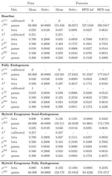
semi-endogenous, and the hybrid exogenous and fully endogenous. Prior choices are kept identical. We have listed the mean estimates of key param-eters governing the growth and innovation dynamics across different model extensions. Additional details and results are reported in Appendix C.4.
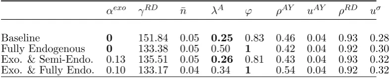
Table 4: Estimated parameters across extensions
αexo γRD n¯ λA ϕ ρAY uAY ρRD uσ
Baseline 0 151.84 0.05 0.25 0.83 0.46 0.04 0.93 0.28 Fully Endogenous 0 133.38 0.05 0.50 1 0.42 0.04 0.92 0.30 Exo. & Semi-Endo. 0.13 135.51 0.05 0.26 0.81 0.43 0.04 0.93 0.32 Exo. & Fully Endo. 0.10 133.17 0.04 0.34 1 0.54 0.04 0.92 0.32
This table reports mean values for estimated parameters. Bold values indicate cali-brated parameters. Values are rounded to the second decimal.
First, consider the estimateαexo for which we have chosen a wide prior.
This parameter describes what share frontier growth is purely exogenous according to our model. In both hybrid extensions which allow for purely exogenous growth the estimated share αexo is small and consistently
esti-mated at around 10−13 percent. Thus, our estimations confirm endoge-nous R&D investment as a key driver of frontier growth. By the same token, the modest share of the exogenous component suggests a strong role for R&D policies. This result is well in line with the estimates of our baseline model. The large intertemporal knowledge spillover parame-ter ϕ implies long-lasting impacts of policies and shocks (such as financial disturbances) affecting R&D dynamics. Moreover, the estimated share of exogenous growth, αexo, should be interpreted as an upper bound: It may,
for instance, also reflect technological spillovers from other countries which we do not explicitly model here.
duplication. In their calibrated model, Jones and Williams (2000) suggest 0.50 as a lower bound of λA. However, as argued before in Section 2.4,
gAY,max
t refers to the growth of frontier productivity, and not to the growth
rate of patents. Consequently, we already account for the effects of patents on productivity growth. This difference in growth accounting explains the relatively low value of λA compared toJones and Williams (2000).
Finally, other estimates of growth and innovation parameters are con-firmed across the extensions considered here. We find high R&D adjust-ment costs and the steady state share of innovating sectors is estimated at around 5 percent per quarter. R&D spillover shocks are large and persis-tent, whereas shocks to R&D investment risk premia are smaller and of a more temporary nature.
5
Conclusion
The macroeconomic experience of the last decade stressed the importance of jointly studying the growth and fluctuations behavior of the economy. In fact, trend and business cycle seemed quite intertwined, suggesting the need to quantify key drivers of these quite complex and unprecedented dy-namics. To that aim we have here built an integrated medium-scale DSGE model featuring a New Keynesian part built upon a rich set of features common to Smets and Wouters (2003) and related literature, as well as a Schumpeterian endogenous and/or semi-endogenous growth engine. To guarantee independence of the long-term growth approach used, we also have allowed the model to nest exogenous growth as a special case, leav-ing it to the data to decide. As in Aghion and Howitt (1992) and Nu˜no
(2011), innovations are the outcome of a patent-race in every sector, with each innovation improving upon existing goods. Innovating firms replace the incumbent monopolist and earn higher profits until the next innovation occurs. Knowledge spillovers push the technological frontier further.
do not explicitly model. Positive mark-up and household savings shocks also contributed to the recent slump. Fiscal and monetary policies could partially offset these adverse shocks.
Our data analysis confirms that the generality of frontier growth in potential GDP is