The Meaning of “Most” for Visual Question Answering Models

46

The meaning of “most” for visual question answering models

Alexander Kuhnle Department of Computer Science

and Technology University of Cambridge Cambridge, United Kingdom

[email protected]

Ann Copestake

Department of Computer Science and Technology

University of Cambridge Cambridge, United Kingdom

[email protected]

Abstract

The correct interpretation of quantifier state-ments in the context of a visual scene requires non-trivial inference mechanisms. For the ex-ample of “most”, we discuss two strategies which rely on fundamentally different cogni-tive concepts. Our aim is to identify what strat-egy deep learning models for visual question answering learn when trained on such ques-tions. To this end, we carefully design data to replicate experiments from psycholinguis-tics where the same question was investigated for humans. Focusing on the FiLM visual question answering model, our experiments indicate that a form of approximate number system emerges whose performance declines with more difficult scenes as predicted by We-ber’s law. Moreover, we identify confounding factors, like spatial arrangement of the scene, which impede the effectiveness of this system.

1 Introduction

Deep learning methods have been very successful in many natural language processing tasks, rang-ing from syntactic parsrang-ing to machine translation to image captioning. However, despite signifi-cantly raised performance scores on benchmark datasets, researchers increasingly worry about in-terpretability and indeed quality of model deci-sions. We see two distinct research endeavors here, one being more pragmatic, forward-oriented, and guided by the question“Can a system solve this task?”, the other being more analytic, reflec-tive, and motivated by the question “How does a system solve this task?”. In other words, the former aspires to improve performance, while the latter aims to increase our understanding of deep learning models.

By ‘understanding’ here we mean observing a reasoning mechanism that, if not human-like, at least is cognitively plausible. This is by no

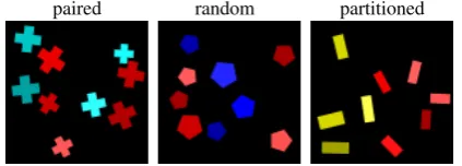
paired random partitioned

“More than half the shapes are red shapes?”

Figure 1: Three types of spatial arrangement of ob-jects which may or may not affect the performance of a mechanism for verifying“most”statements. Going from left to right, a strategy based on pairing entities of each set and identifying the remainder presumably gets more difficult, while a strategy based on comparing set cardinalities does not.

means necessary for practically solving a task, however, we highlight two reasons why being able to explain model behavior is nonetheless impor-tant: On the one hand, cognitive plausibility in-creases confidence in the abilities of a system – one is generally more willing to rely on a reason-able than an incomprehensible mechanism. On the other hand, pointing out systematic shortcomings inspires systematic improvements and hence can guide progress. Moreover, particularly in the case of a human-centered domain like natural language, ultimately, some degree of comparability to hu-man perforhu-mance is indispensable.

In this paper we are inspired by experimen-tal practice in psycholinguistics to shed light on the question how deep learning models for visual question answering (VQA) learn to interpret state-ments involving the quantifier“most”. We follow

We want to emphasize the experimental ap-proach and its difference to mainstream ma-chine learning practice. For different verification strategies, conditions are identified that should or should not affect their performance, and test in-stances are designed accordingly. By comparing the accuracy of subjects on various instance pat-terns, predictions about a subject’s performance for these mechanisms can be verified and the most likely explanation identified. Note that our advo-cated evaluation methodology is entirely extrin-sic and does not constrain the system in any way (like requiring attention maps) or require a specific framework (like being probabilistic).

Psychology as a discipline has focused entirely on questions around how humans process situa-tions and arrive at decisions, and consequently has the potential to inspire a lot of experiments (like ours) for investigating the same questions in the context of machine learning. Similar to psychol-ogy, we advocate the preference of an artificial experimentation environment which can be con-trolled in detail, over the importance of data orig-inating from the real world, to arrive at more con-vincing and thus meaningful results.

It is less common recently to evaluate deep learning models on artificial data tailored to a specific problem, as opposed to big real-world datasets. However, artificial data has a history in deep learning of establishing new techniques – most prominently, LSTMs were introduced by showing their ability to handle various formal grammars (Gers and Schmidhuber, 2001) – and our higher-level goal with this paper is to demon-strate the potential for more informative evalua-tion of machine learning models in general. This is motivated by our belief that, in the long term, true progress can only be made if we do not just rely on the narrative of neural networks “learning to understand/solve”a task, but can actually confirm our theories experimentally. Taking inspiration from psychology seems particularly appropriate in the context of powerful deep learning models, which recently are not infrequently described by anthropomorphizing words like“understanding”, and compared to“human-level”performance.

2 The meaning of “most”

In this section we will discuss two mechanisms of interpreting“most”and introduce relevant cogni-tive concepts.

2.1 Generalized quantifiers and “most”

“Most” has a special status in linguistics due to the fact that it is the most prominent example of a quantifier whose semantics cannot be expressed in first-order logic, while other simple natural lan-guage quantifiers like “some”, “every” or “no” directly correspond to the quantifier primitives∃

and∀ (plus logical operators ∧, ∨ and¬). This situation is not just a matter of introducing further appropriate primitives, but requires a fundamental extension of the logic system and its expressivity.

In the following, by x we denote an entity, A

andBdenote predicates (“square”,“red”),A(x)

is true if and only ifxsatisfiesA, andSA ={x : A(x)}is the corresponding set of entities satisfy-ing this predicate (“squares”). Thus we can define the semantics of“some”and“every”:

some(A, B)⇔ ∃x:A(x)∧B(x)

every(A, B)⇔ ∀x:A(x)⇒B(x)

Importantly, these definitions do not involve the concept of set cardinality and indeed can be for-mulated without involving sets. This is not possi-ble for“most”, which is commonly defined in one of the following ways:

most(A, B)⇔ |SA∧B|>1/2· |A|

⇔ |SA∧B|>|SA∧¬B| (1)

This makes “most” an example of ageneralized quantifier, and in fact all generalized quantifiers can be defined in terms of cardinalities, indicating the apparent importance of a cardinality concept to human cognition.

2.2 Alternative characterization

There is another way to define“most”which uses the fact that whether two sets are equinumerous can be determined without a concept of cardinal-ity, but based on the idea of a bijection:

A↔B :⇔ ∀x:A(x)⇔B(x)

⇔ |SA|=|SB|

The definition of equinumerosity can be general-ized to“more than”(and, correspondingly, “less than”), which lets us define“most”as follows:

most(A, B)⇔ ∃S (SA∧B :S↔SA∧¬B (2)

2.3 Two interpretation strategies

These two characterizations are of course truth-conditionally equivalent, that is, every situation in which one of them holds, the other holds, and vice versa. In particular, if we are just interested in solving a task involving“most”statements, we can be agnostic about which definition our system prefers. Nevertheless, the subtle differences be-tween these two characterizations suggest differ-ent algorithmic mechanisms of verifying or falsi-fying such statements, meaning that a system pro-cesses a visual scene differently to come to the (same) conclusion about a statement’s truth.

Characterization (1) represents the cardinality-based strategyof interpreting“most”:

1. Estimate the number of entities satisfying both predicates (“red squares”) and the num-ber satisfying one predicate but not the other (“non-red squares”).

2. Compare these number estimates and check whether the former is greater than the latter.

We want to add that, actually, the two defini-tions in (1) already suggest a minor variation of this mechanism – see Hackl(2009) for a discus-sion on “most” versus“more than half ”. How-ever, we do not focus on this detail here, and as-sume the second variant in (1) to be ‘strictly’ sim-pler in the sense that both involve estimating and comparing cardinalities, but the first variant addi-tionally involves the rather complex operation of halving one number estimates.

Characterization (2) utilizes the concept of a bi-jection, which is a comparatively simple pairing mechanism and as such could be imagined to be a primitive cognitive operation. This gives us the

pairing-based strategyof verifying“most”:

1. Successively match entities satisfying both predicates (“red squares”) uniquely with en-tities satisfying one predicate but not the other (“non-red squares”).

2. The remaining entities are all of one type, so pick one and check whether it is of the first type (“red square”).

2.4 Cognitive implications

Finding evidence for one strategy over the other has substantial implications with respect to the ‘cognitive abilities’ of a neural network model. In

particular, evidence for a cardinality-based pro-cessing of “most” suggests the existence of an

approximate number system (ANS), which is able to simultaneously estimate the number of ob-jects in two sets, and perform higher-level op-erations on the resulting number representations themselves, like the comparison operation here. Explicit counting would be an even more accurate mechanism here, but neither available to the sub-jects in the experiments ofPietroski et al. (2009) due to very short scene display time, nor likely to be learned by the ‘one-glance’ feed-forward-style neural network we evaluate in this work1.

The ANS (see appendix in Lidz et al. (2011) for a summary) is an evolutionary comparatively old mechanism which is shared between many dif-ferent species throughout the animal world. It emerges without explicit training and produces ap-proximate representations of the number of ob-jects of some type. They are approximate in the sense that their number judgment is not ‘sharp’, but resulting behavior exhibits variance – like in-terpreting “most” statements with a cardinality-based strategy, as described above. This vari-ance follows Weber’s law which states that the discriminability of two quantities is a function of their ratio2. The precision of the ANS is thus usu-ally indicated by a characteristic value called We-ber fractionwhich relates quantity and variance. The ANS of a typical adult human is often re-ported to have a Weber fraction of 1.14 or, more tangibly, it can distinguish a ratio of 7:8 with 75% accuracy. Finding evidence for the emergence of a similar system in deep neural networks indicates that these models can indeed learn more abstract concepts (approximate numbers) than mere super-ficial pattern matching (“red squares”etc).

1

By“one-glance feed-forward-style networks”we refer to the predominant type of network architecture which, by de-sign, consists of a fixed sequence of computation steps before arriving at a decision. In particular, such models do not have the ability to interact with their input dynamically depending on the complexity of an instance, or perform more general recursive computations beyond the fixed recurrent modules built into their design. Important for the discussion here is the fact that precise – in contrast to approximate or subitizing-style – counting is by definition a recursive ability, thus im-possible to learn for such models.

2

Both mechanisms to interpret “most” suggest conditions in which they should perform well or badly. For the cardinality-based one, the dif-ference in numbers of the two sets in question is expected to be essential: smaller differences, or greater numbers for the same absolute differ-ence, require more accurate number estimations and hence make this comparison harder, accord-ing to Weber’s law. The pairing-based mecha-nism, on the other hand, is likely affected by the spatial arrangement of the objects in question: if the objects are more clustered within one set, pair-ing them with objects from the other set becomes harder. Importantly, these conditions are orthogo-nal, so each mechanism should not substantially be affected by the other condition, respectively. By constructing (artificial) scenes where one of the conditions dominates the configuration, and mea-suring the accuracy of being able to correctly inter-pret propositions involving “most”, the expected difficulties can be confirmed (or refuted) and thus indicate which mechanism is actually at work.

Using this methodology,Pietroski et al.(2009) show that humans exhibit a default strategy of in-terpreting“most”, at least when only given 200ms to look at the scene and hence having to rely on an immediate subconscious judgment. This strategy is based on the approximate number system and the cardinality-based mechanism. Moreover, the behavior is shown to be sub-optimal in some situa-tions where humans would, in principle, be able to perform better if deviating from their default strat-egy. Since machine learning models are trained by optimizing parameters for the task at hand, it is far from obvious whether they learn a similarly stable default mechanism, or instead follow a po-tentially superior adaptive strategy depending on the situation. While the latter is likely more effi-cient in solving at least a narrowly defined task, the former would instead suggest that the system is able to acquire and utilize core concepts like an approximate number system.

We may speculate about the innate preference of modern network architectures for either of the strategies: Most of the visual processing is based on convolutions which, being an inherently local computation, we assume would favor the pairing-based strategy via locally matching and ‘can-celling out’ entities of the two predicates. On the other hand, the tensors resulting from the sequence of convolution operations are globally fused into

a final embedding vector, which in turn would support the more globally aggregating cardinality-based strategy. However, the type of computa-tions and representacomputa-tions learned by deep neu-ral networks are poorly understood, making such speculations fallacious. We thus emphasize again that the higher-level motivation for this paper is to demonstrate how we need not rely on such specu-lative ‘narratives’, but can experimentally substan-tiate our claims.

3 Experimental setup

The setup in this paper closely resembles the psychological experiments conducted byPietroski et al.(2009), but aimed at a state-of-the-art VQA model and its interpretation of“most”.

3.1 Training and evaluation data

We use the ShapeWorld framework (Kuhnle and Copestake,2017) as starting point to generate ap-propriate data. ShapeWorld is a configurable gen-eration system for abstract, visually grounded lan-guage data. A data point consists of an image, an accompanying caption, and an agreement value in-dicating whether the caption is true given the im-age. The underlying task, image caption agree-ment, essentially corresponds to yes/no questions and as such is a type of visual question answering. Internally, the system samples an abstract world description from which a semantic caption repre-sentation is extracted. Both are then turned into ‘natural’ (but still abstract) representations as im-age and natural languim-age statement, respectively. The latter transformation is based on a semantic grammar formalism (see the paper for details).

We use the pre-implemented quantifier cap-tioner component, both in its unrestricted ver-sion and one with available quantifiers restricted to “more than half ” and “less than half ”3. The former contains various additional (gener-alized) quantifiers (“no”, “a/three quarter(s)”, “a/two third(s)”, “all”) and numbers (ranging from“zero”to“five”), each in combination with a comparing modifier (“less than”,“at most”, “ex-actly”,“at least”,“more than”,“not”). We refer to the unrestricted version as Q-full, the other one

3

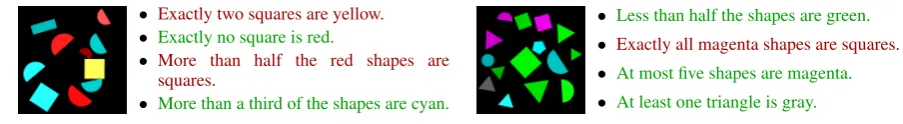
• Exactly two squares are yellow. • Exactly no square is red.

• More than half the red shapes are

squares.

• More than a third of the shapes are cyan.

• Less than half the shapes are green. • Exactly all magenta shapes are squares.

• At most five shapes are magenta.

• At least one triangle is gray.

Figure 2: Two example images with in-/correct captions, taken from the Q-full dataset (all quantifiers/numbers).

as Q-half. Figure 2 shows two images together with potential Q-full captions.

We also use the default world generator to pro-duce training data (up to 15 randomly positioned objects, as seen in figure 2). However, all of the pre-implemented generator modules are too generic for our evaluation purposes, since they do not allow to control attributes and positioning of objects to the desired degree. We thus imple-mented our own custom generator module with the following functionality to produce test data.

Attribute contrast: For each instance, either the attribute ‘shape’ or ‘color’ is picked4, and subsequently two values for this attribute and one value for the other is randomly chosen. This means that the only relevant difference between objects in every image is either one of two shape or color values (for instance, red vs blue squares, or red squares vs circles).

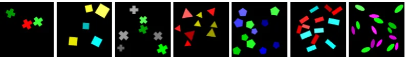
Contrast ratios: A list of valid ratios between the contrasted attributes can be specified, from which one will randomly be chosen per in-stance. For instance, a ratio of 2:3 means that there are 50% more objects with the sec-ond than the first attribute. We look at values close to 1:1, that is, 1:2, 2:3, 3:4, 4:5, etc. The increasing difficulty (for humans) result-ing from closer ratios is illustrated in figure

3. Multiples of the smaller-valued ratios are also generated (e.g., 2:4 or 6:9), within the limit of up to 15 objects overall.

Area-controlled (vs size-controlled): If this op-tion is set, object sizes are not chosen uni-formly across the entire valid range, but size ranges for the two contrasting object types are adapted to the given contrast ratio and size of the chosen shape(s), so that both at-tributes cover the same image area on av-erage. This means that the more numer-ous attribute will generally be represented by

4_{Note that we chose the examples in figures to always}

vary in color only, for clarity.

smaller objects, and the difference in covered area between, for instance, squares and trian-gles is taken into account.

While objects are still positioned randomly in the basic version of this new generator module, we define two modes which control this aspect as well. Figure 1 in the introduction illustrates the different modes.

Partitioned positioning: An angle is randomly chosen for each image, and objects of the contrasting attributes are consistently placed either on one side or the other.

Paired positioning: If there are objects of the contrasted attribute which are not yet paired, one of them is randomly chosen and the new object is placed next to it.

The captions of these evaluation instances are always of the form “More/less than half the shapes are X”. with “X” being the attribute in question, for instance,“squares”or“red shapes”. Note that this is an even more constrained cap-tioner than the one used for Q-half. We also em-phasize that, in contrast to this new evaluation generator module, the default generator configu-ration of the ‘quantification’ dataset pre-specified in ShapeWorld is used to generate the training in-stances in Q-half and Q-full. So these images gen-erally contain many more than just two contrasted attributes, and ratios between attributes tend to be accordingly smaller. The examples in figure2are chosen to illustrate this fact: the second example contains a“half ”statement with ratio 7:8, and the first contains one about a 0:4 ratio, while the im-age would also allow for a more ‘interesting’ 3:4 ratio (color of semicircles).

Figure 3: From left to right, the ratio between the two attributes is increasingly balanced.

system to actually learn the fact that shape and color are attributes that can be combined in any way, instead of just straightforward binary pattern matching. Note that the humans in the psycho-logical experiments have learned language in even more complex situations, which we cannot hope to approximate here. Moreover, our data does not contain yes/no questions but true/false captions, and“most”-equivalent variations“more/less than half ”. Since the model is trained from scratch on such data, this should not affect results.

We do not implement the ‘column pairs mixed/sorted’ modes since they would require comparatively big and mostly empty images, hence require bigger networks and might cause practical learning problems due to sparseness, which we do not want to address here. In con-trast, our ‘partitioned’ mode is more difficult than the ones investigated byPietroski et al.(2009), at least for a pairing-based mechanism.

3.2 Model

We focus on the FiLM model (Perez et al.,2018) here since it showed close-to-perfect accuracy on the CLEVR dataset (Johnson et al., 2017a). We interpret the ShapeWorld captions and agreement values as questions and answer, respectively. The image is processed using either a pre-trained CNN or a four-layer CNN trained from scratch on the task. The question is processed by a GRU. In a sequence of four residual blocks, the image infor-mation is processed with its features linearly mod-ulated (scale, offset) conditioned on the processed question embedding. Finally, the classifier module produces the answer, true or false. We use the code made available by the authors of the FiLM model, without changing any parameters. The only aspect we adapt is the trainable four-layer CNN, which uses a kernel size of 3, batch normalization and a stride of 2 in the second and fourth layer.

We considered investigating other models as well: The PG+EE model (Johnson et al., 2017b) is openly available and achieved very good per-formance on CLEVR, however, it relies on the

‘program tree’ provided by CLEVR, and while there exists a basic conversion of ShapeWorld cap-tion models to CLEVR program trees, first, the CLEVR-specific modules do not cover quantifiers like“most”and, second, these program trees en-code the interpretation strategy, which would de-feat the purpose of our investigation to analyze precisely this mechanism as learned from data. The RelationNet architecture (Santoro et al.,2017) explicitly implements a pairing-based mechanism and hence we considered its evaluation less inter-esting than FiLM. For similar reasons, we did not focus on the VQA model ofZhang et al. (2018), whose architecture includes an explicit counting component. While our aim is to investigate the strategy for understanding “most” learned from data, it would be interesting to examine in both cases whether their architectural prior does in-deed have the expected effect. Finally, we only learned about the MAC model (Hudson and Man-ning,2018) after we started this project and so de-cided to leave it for future work, but we definitely consider it one of the most interesting candidate models to evaluate, since its architecture does not suggest an obvious preference for either strategy.

3.3 Training details

The training set for both Q-full and Q-half consists of around 100k (25x 4096) images with 5 captions per image, so overall around 500k instances. The model is trained for 100k iterations with a batch size of 64. Training performance is measured on an additional validation set of 20k instances. Moreover, we produced 1024 instances for each of the overall 48 evaluation configurations, to in-vestigate the trained model in more detail.

4 Results

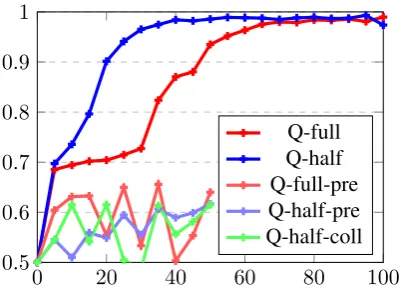
Perfor-mance of the system over the course of the 100k training iterations is shown in figure 4. The two models, referred to by Q-full and Q-half below, learn to solve the task quasi-perfectly, with a final accuracy of 98.9% and 99.4% respectively. Not surprisingly, the system trained on the more di-verse Q-full training set takes longer to reach this level of performance, but nevertheless plateaus af-ter around 70k iaf-terations.

For the sake of completeness, we also include the performance of other models in this figure, which failed to show clear improvement over the first 50k iterations. This includes the FiLM model with pre-trained instead of trainable CNN module (full-pre, half-pre), and an earlier trial on Q-half (Q-Q-half-coll) where we did not constrain the data generation to not produce object collisions (the default in ShapeWorld is to allow up to 25% area overlap). We note, however, that we have not done any hyperparameter search which might al-leviate these learning problems.

Evaluation. Table 5 presents a detailed break-down of system performance on the evaluation set-tings. Before discussing the results in detail, we want to reiterate three key differences between the evaluation data and the training data:

• The visual scenes here do all exhibit close-to-balanced contrast ratios, while this is not the case for the training instances.

• The evaluation scenes only contain objects of two different attribute pairs, and conse-quently the numbers to compare are generally greater than in the training instances, where more attributes are likely present in a scene.

• Q-full contains not just statements involving “half ”– in fact, a random sample of 100 im-ages / 500 captions suggests that they consti-tute only around 8% of the dataset (and this includes combinations with modifiers beyond “more/less than”).

Considering that, the relatively high accuracy on test instances throughout indicates a remarkable degree of generalization.

More balanced ratios. The most consistent ef-fect is that more balanced ratios of contrasted at-tributes cause performance to decrease. This is certainly affected by the tendency of the training data to not include many examples of almost bal-anced ratios. However, if this were the only

rea-0 20 40 60 80 100 0.5

0.6 0.7 0.8 0.9 1

Q-full Q-half Q-full-pre Q-half-pre Q-half-coll

Figure 4: Training performance (iterations in 1000). Q-full: unconstrained dataset; Q-half: dataset restricted to“less/more than half ”;-pre: using pre-trained CNN module;-coll: allowing object overlap.

son, one would expect a much more sudden and less uniformly linear decrease. More importantly, since Q-full generally contains fewer“half ” state-ments, the decline should be more pronounced here. We do not observe either of these effects, and thus conclude that both models may actually have developed an approximate number system. This is further discussed at the end of this section.

Random vs paired vs partitioned. There is a clear negative effect of the partitioned configura-tion on performance for the model trained on Q-full, which suggests that the learned mechanism is not robust to a high degree of per-attribute cluster-ing. This indicates at most a weak preference to-wards a pairing-based strategy for Q-full, though, since otherwise the model would not be expected to perform best on the random configuration. In-terestingly, the results for Q-half even suggest slightly better performance on the area-controlled partitioned configuration. Overall, no clear prefer-ence for either the perfectly clustered partitioned or the perfectly mixed paired arrangement is ap-parent. We note, however, that the random mode instances are most similar to the random place-ment of objects in the training data, which might cause this effect.

train mode size-controlled area-controlled

all 1:2 2:3 3:4 4:5 5:6 6:7 7:8 all 1:2 2:3 3:4 4:5 5:6 6:7 7:8

Q-full

random 92 100 99 97 94 91 88 85 93 100 99 97 93 91 86 82

paired 93 99 99 96 93 90 88 82 93 99 99 96 91 87 84 80

part. 89 100 99 92 90 81 77 72 89 99 98 92 88 82 78 72

Q-half

random 92 100 100 98 93 88 88 87 93 100 100 97 92 86 85 82

paired 92 100 100 96 90 86 84 79 92 100 99 96 87 84 79 76

part. 91 100 99 96 86 83 83 80 91 100 99 94 89 83 83 80

Figure 5: Accuracy in percent of the models trained on Q-full and Q-half for the various evaluation configurations.

model(s) learn to use covered area as a feature to inform a correct decision in some cases.

Q-full vs Q-half. There seems to be a ten-dency of the system trained on Q-full to perform marginally better, except for the partitioned mode discussed before. The fact that this model per-forms at least on a par with the one trained on Q-half, while only seeing a fraction of directly rel-evant training captions, indicates that the learning process is not ‘distracted’ by the variety of cap-tions, and indeed might profit from it.

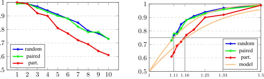
Ratios and Weber fraction. We generated eval-uation sets of even more balanced ratios (8:9, 9:10, 10:11, increasing the overall number of objects accordingly to 17/19/21), and in figure 6 plotted the accuracy of the Q-full model on increasingly balanced sets for all three spatial configuration modes, not controlling for area (which for greater numbers only has a negligible effect anyway). The figure also contains a diagram with accuracy plot-ted against ratio fraction, which is more common in the context of Weber’s law. The characteristic Weber fraction can be read off directly as the ratio at which a subject is able to distinguish two val-ues with 75% accuracy. We observe around 1.11 for random/paired and 1.16 for partitioned, which corresponds to 9:10 and 6:7 as closest integer ra-tios. These values are in the same region as the average human Weber fraction, which is often re-ported as being 1.14, or 7:8.

We emphasize that these curves align well with the trend predicted by Weber’s law, even for the ratios with more than 15 objects overall, where such situations have never been encountered dur-ing traindur-ing. All this strongly suggests that the model learns a mechanism similar to an ANS, which is able to produce representations that can (at least) be utilized for identifying the more nu-merous set. It can in particular be concluded that the system does not actually learn to explicitly

count, since we would then not expect to observe such fuzziness characteristic to an ANS.

Moreover, since performance is affected some-what by the partitioned and the area-controlled modes, the interpretation of“most” seems to be informed by other features as well. As we noted earlier, since the model is trained to optimize this task, an adaptive strategy is not unexpected. On the contrary, more surprising is the fact that an ANS-like system emerges as a dominating ‘back-bone’ mechanism, with additional factors acting as less influential ‘secondary’ features.

5 Related work

Visual question answering (VQA) is the general task of answering questions about visual scenes. Since the introduction of the VQA Dataset (Antol et al.,2015), this dataset was widely used as evalu-ation benchmark for multimodal deep learning. It provides a shallow categorization of questions, in-cluding basic count questions, however, these cat-egories are far too coarse for our purposes.

Motivated by various problems with the VQA Dataset (Goyal et al.,2017;Agrawal et al.,2016), a range of artificial abstract datasets have been in-troduced recently. CLEVR (Johnson et al.,2017a) consists of rendered images of geometric objects and questions generated based on templates, cov-ering some abilities like number or attribute com-parison in more detail, but still in a fixed catego-rization. NLVR (Suhr et al.,2017) contains crowd-sourced statements about abstract images, but does not sort them according to some criteria. Recently, the COG dataset (Yang et al., 2018) was intro-duced, which most explicitly focuses on replicat-ing psychological experiments for deep learnreplicat-ing models, hence most related to our work. However, their dataset does not contain any number or quan-tifier statements.

1 2 3 4 5 6 7 8 9 10 0.5

0.6 0.7 0.8 0.9 1

random paired

part.

1 1.11 1.16 1.25 1.33 1.5 0.5

0.6 0.7 0.8 0.9 1

random paired

part. model

Figure 6:Left:Q-full model performance for increasingly balanced ratios (x-axis indicates ratio via n:n+1).

Right:Performance as a function of the actual ratio fraction (n+1)/n, with Weber fraction (75%) highlighted.

psychologically inspired viewpoint. Stoianov and Zorzi (2012) find that visual numerosity emerges from unsupervised learning on abstract image data. Zhang et al. (2015) look at salient object subitizing in real-world images, formulated as a classification task over five classes ranging from “0” to “4 or more”. In a more general number-per-category classification setup, Chattopadhyay et al. (2017) investigate different methods of ob-taining counts per object category, including one which is inspired by subitizing. Moving beyond explicit number classification, (Zhang et al.,2018) recently introduced a dedicated counting module for visual question answering.

Other work looks at a similar classification task, but for proper quantifiers like “no”, “few”, “most”, “all”, first on abstract images of circles (Sorodoc et al., 2016), then on natural scenes (Sorodoc et al., 2018). Recently,Pezzelle et al. (2018) in-vestigated a hierarchy of quantifier-related clas-sification abilities, from comparatives via quan-tifiers like the ones above to fine-grained pro-portions. Wu et al. (2018), besides investigat-ing precise numerosity via number classification as above, also look at approximate numerosity as binary greater/smaller decision, which closely cor-responds to our experiments. However, on the one hand, their focus is on the subitizing ability, not the approximate number system. On the other hand, their experiments follow a different methodology in that they already train models on specifically designed datasets, while we deliberately leverage such targeted data only for evaluation.

On a methodological level, our proposal of in-spiring experimental setup and evaluation practice for deep learning by cognitive psychology is in line with that ofRitter et al.(2017) and their shape bias investigation for modern vision architectures.

6 Conclusion

We identify two strategies of algorithmically in-terpreting “most” in a visual context, with dif-ferent implications on cognitive concepts. Fol-lowing experimental practice of similar investiga-tions with humans in psycholinguistics, we de-sign experiments and data to shed light on the question whether the state-of-the-art FiLM VQA model shows preference for one strategy over the other. Performance on various specifically de-signed instances does indeed indicate that a form of approximate number system is learned, which generalizes to more difficult scenes as predicted by Weber’s law. The results further suggest that ad-ditional features influence the interpretation pro-cess, which are affected by the spatial arrange-ment and relative size of objects in a scene. There are many opportunities for future work from here, from strengthening the finding of an approximate number system and further analyzing confound-ing factors to investigatconfound-ing the relation to more ex-plicit counting tasks.

Acknowledgments

We thank the anonymous reviewers for their con-structive feedback. AK is grateful for being sup-ported by a Qualcomm Research Studentship and an EPSRC Doctoral Training Studentship.

References

Aishwarya Agrawal, Dhruv Batra, and Devi Parikh. 2016. Analyzing the behavior of visual question answering models. In Proceedings of the Confer-ence on Empirical Methods in Natural Language Processing, EMNLP 2016, pages 1955–1960.

and Devi Parikh. 2015. VQA: Visual question an-swering. InProceedings of the IEEE International Conference on Computer Vision, ICCV 2015.

Prithvijit Chattopadhyay, Ramakrishna Vedantam, Ramprasaath R. Selvaraju, Dhruv Batra, and Devi Parikh. 2017. Counting everyday objects in every-day scenes. InProceedings of the IEEE Conference on Computer Vision and Pattern Recognition, CVPR 2017, pages 4428–4437.

Felix A. Gers and J¨urgen Schmidhuber. 2001. LSTM recurrent networks learn simple context-free and context-sensitive languages. Transactions on Neu-ral Networks, 12(6):1333–1340.

Yash Goyal, Tejas Khot, Douglas Summers-Stay, Dhruv Batra, and Devi Parikh. 2017. Making the V in VQA matter: Elevating the role of image un-derstanding in Visual Question Answering. In Pro-ceedings of the IEEE Conference on Computer Vi-sion and Pattern Recognition, CVPR 2017, pages 6325–6334.

Martin Hackl. 2009. On the grammar and processing of proportional quantifiers: most versus more than half. Natural Language Semantics, 17(1):63–98.

Drew A. Hudson and Christopher D. Manning. 2018. Compositional attention networks for machine rea-soning. InProceedings of the International Confer-ence on Learning Representations, ICLR 2018.

Justin Johnson, Bharath Hariharan, Laurens van der Maaten, Li Fei-Fei, C. Lawrence Zitnick, and Ross Girshick. 2017a. CLEVR: A diagnostic dataset for compositional language and elementary visual rea-soning. InProceedings of the IEEE Conference on Computer Vision and Pattern Recognition, CVPR 2017.

Justin Johnson, Bharath Hariharan, Laurens van der Maaten, Judy Hoffman, Li Fei-Fei, C Lawrence Zit-nick, and Ross Girshick. 2017b. Inferring and ex-ecuting programs for visual reasoning. In Proceed-ings of the IEEE International Conference on Com-puter Vision, ICCV 2017.

Alexander Kuhnle and Ann Copestake. 2017. Shape-World - A new test methodology for multimodal lan-guage understanding. ArXiv e-prints 1704.04517.

Jeffrey Lidz, Paul Pietroski, Justin Halberda, and Tim Hunter. 2011. Interface transparency and the psy-chosemantics of most. Natural Language Seman-tics, 19(3):227–256.

Ethan Perez, Florian Strub, Harm de Vries, Vincent Dumoulin, and Aaron C. Courville. 2018. FiLM: Visual reasoning with a general conditioning layer. InAAAI.

Sandro Pezzelle, Ionut-Teodor Sorodoc, and Raffaella Bernardi. 2018. Comparatives, quantifiers, propor-tions: A multi-task model for the learning of quan-tities from vision. InProceedings of the Conference

of the North American Chapter of the Association for Computational Linguistics, NAACL 2018.

Paul Pietroski, Jeffrey Lidz, Tim Hunter, and Justin Halberda. 2009. The meaning of ’most’: Semantics, numerosity and psychology. Mind and Language, 24(5):554–585.

Samuel Ritter, David G. T. Barrett, Adam Santoro, and Matt M. Botvinick. 2017. Cognitive psychology for deep neural networks: A shape bias case study. In

Proceedings of the 34th International Conference on Machine Learning, ICML 2017, pages 2940–2949.

Adam Santoro, David Raposo, David G. T. Bar-rett, Mateusz Malinowski, Razvan Pascanu, Peter Battaglia, and Timothy P. Lillicrap. 2017. A sim-ple neural network module for relational reasoning. InProceedings of the Annual Conference on Neural Information Processing Systems, NIPS 2017, pages 4974–4983.

Ionut Sorodoc, Angeliki Lazaridou, Gemma Boleda, Aur´elie Herbelot, Sandro Pezzelle, and Raffaella Bernardi. 2016. “Look, some green circles!”: Learning to quantify from images. InProceedings of the 5th Workshop on Vision and Language, Berlin, Germany.

Ionut Sorodoc, Sandro Pezzelle, Aur´elie Herbelot, Mariella Dimiccoli, and Raffaella Bernardi. 2018. Learning quantification from images: A structured neural architecture. Natural Language Engineering, page 130.

Ivilin Stoianov and Marco Zorzi. 2012. Emergence of a ‘visual number sense’ in hierarchical generative models. Nature Neuroscience, 15(194):194–196.

Alane Suhr, Mike Lewis, James Yeh, and Yoav Artzi. 2017. A corpus of natural language for visual rea-soning. In Proceedings of the 55th Annual Meet-ing of the Association for Computational LMeet-inguis- Linguis-tics, ACL 2017.

Xiaolin Wu, Xi Zhang, and Xiao Shu. 2018. On numerosity of deep convolutional neural networks.

ArXiv e-prints 1802.05160.

Guangyu Robert Yang, Igor Ganichev, Xiao-Jing Wang, Jonathon Shlens, and David Sussillo. 2018. A dataset and architecture for visual reasoning with a working memory. ArXiv e-prints 1803.06092.

Jianming Zhang, Shuga Ma, Mehrnoosh Sameki, Stan Sclaroff, Margrit Betke, Zhe Lin, Xiaohui Shen, Brian Price, and Radom´ır Mˇech. 2015. Salient ob-ject subitizing. InProceedings of the IEEE Confer-ence on Computer Vision and Pattern Recognition, CVPR 2015.