Does financial sector development affect the growth gains from trade opennes?

(1)

Munich Personal RePEc Archive

Does financial sector development affect

the growth gains from trade opennes?

Ramírez-Rondán, N. R. and Terrones, Marco E. and Vilchez,

Andrea

Universidad del Pacifico

November 2018

(2)

Does financial sector development affect

the growth gains from trade openness?

∗

N.R. Ram´ırez-Rond´an

Universidad del Pac´ıfico

Marco E. Terrones

Andrea Vilchez

November, 2018

Abstract

A sizeable literature suggests that financial sector development could be an important enabler of the growth benefits of trade openness. We provide a com-prehensive analysis of how financial development can affect the relationship be-tween trade openness and growth using a dynamic panel threshold model and an extensive dataset for a large sample of countries for the 1970-2015 period. We find that there is a financial development threshold in which trade openness has a positive and significant effect on economic growth. We also find that when splitting the sample into industrialized and non-industrialized countries, the fi-nancial development threshold that enables the growth benefits of trade is higher in the former group of countries than in the latter. This finding is consistent with the fact that the export composition of industrialized countries is tilted towards more capital-intensive finance-constrained goods.

JEL Classification: F43, O41, C33

Key words: Trade openness, growth, threshold model, panel data.

∗_{We are grateful to Roberto Chang and Diego Winkelried as well as the participants of the Ninth}

conference on Growth and Business Cycle in Theory and Practice (Manchester, United Kingdom); the 2018 Congress of the Peruvian Economic Association (Piura, Peru); the 2018 Annual Meeting of the Economics Society of Chile (Valparaiso, Chile); the Global Research on Emerging Economies Confer-ence (Lima, Peru), and the Universidad del Pac´ıfico Research Seminar for their valuable comments and suggestions. As usual, all remaining errors are ours.

(3)

1

Introduction

A key issue in economic growth is whether or not trade openness has significant growth effects and how these effects are best enabled. In theory, there are many channels through which trade openness can have positive effects on growth. For instance, it has been argued that openness generates important gains from comparative advantage, dis-seminates knowledge and technologies, facilitates technology transfer, increases mar-ket size, and reduces rent-seeking activities (Grossman and Helpman,1991; Jones and Romer,2010;Young,1991, among others). These effects should, in turn, be reflected in stronger economic growth as resource allocation improves and the frontier of production expands. Trade openness, however, could also be detrimental to growth, particularly when a country specializes in extractive and non-innovative sectors (Matsuyama,1992;

Chang et al.,2009, among others).

The empirical evidence of a strong and robust link between trade openness and growth is, unsurprisingly, mixed. On the one hand, cross-country and panel data stud-ies have found that trade has a positive effect on growth (Dollar, 1992;Edwards,1998;

Frankel and Romer,1999; Leeet al., 2004;Wacziarg and Welch,2008, among others). Some of these studies, however, have been criticized for their use of faulty methodolo-gies, inadequate trade openness measures, and lack of robust results (Rodr´ıguez and Rodrik, 2001; Rodr´ıguez, 2007). On the other hand, other studies have reported ev-idence that trade openness in itself might not be enough to deliver strong economic growth and that the trade and growth relationship might even be nonlinear (Ula¸san,

2015; Chang et al., 2009). Openness seems to be more effective when complemented by competitiveness-boosting factors.

This latter result suggests that enabling the growth benefits of trade might require the presence of certain institutions, which themselves are a source of comparative ad-vantage (Nunn and Trefler, 2014). One such institution is financial markets. Financial markets are key as they facilitate the interplay between saving and investment deci-sions, and thus economic growth. These markets are, however, fraught with imperfec-tions, asymmetric information, and other problems. The extent of these imperfections affects economic outcomes. The development of financial markets and associated in-stitutions would be reflected in better saving-investment allocation and better growth performance (McKinnon, 1973;Levine, 2005).

(4)

uncovered vanishing (Rousseau and Watchel,2011) and even detrimental growth effects of excessive financial development (Arcand et al., 2015). This latter finding suggests that some countries might have encouraged the development of excessively large fi-nancial sectors. Other studies have used microdata to provide evidence that countries with more developed financial sectors have higher production levels in the externally financed sector (Rajan and Zingales, 1998).

In this paper, we examine whether financial sector development affects the openness and economic growth nexus. This is an extremely topical issue, especially given the pushback against trade openness and the recent introduction of tariffs in some coun-tries, which have made global trade relations increasingly problematic. In addition, important questions about the soundness of developing large financial markets –and the sense that there is too much finance in some countries– have been raised. While we do not address these issues directly, we do examine how financial sector development can strengthen the openness and growth relationship. Are there some threshold levels of financial development that an economy needs to enable the growth benefits from openness? Are these thresholds different across country groups?

There are many ways in which financial development could affect the trade openness and growth nexus. First, financial development can itself be a source of comparative advantage. More developed financial sectors tend to be of most benefit to those indus-tries that require external financing in greater proportion, and affect a country’s trade structure (Rajan and Zingales, 1998; Kletzer and Bardhan, 1987; Beck, 2002, among others). Beck(2002), for instance, reports evidence that countries with more developed financial sectors have a comparative advantage in manufacturing, as the financing of the considerable fixed costs faced by this sector is cheaper in such countries.

Second, financial development, insofar as it mitigates the distortive effects of fi-nancial frictions, can positively affect productivity and tilt trade composition towards capital-intensive industries. Thus, sectors vulnerable to financial frictions, like the large-scale manufacturing sector, respond positively to the development of a country’s financial markets (Bueraet al.,2011). This could lead to a restructuring of a country’s trade composition away from labor-intensive industries and towards capital-intensive industries (Leibovici,2018), including the large-scale manufacturing and high-tech sec-tors. There is some evidence that a country’s export composition matters for economic growth (Hausmannet al., 2007).

(5)

that asset markets allow for well-diversified incomes across a country’s population, protectionist lobbying efforts would be reduced (Feeney and Hillman,2004). Empirical evidence about the complementarity between asset development and trade liberaliza-tion is reported in Svaleryd and Vlachos (2002), andFeeney and Hillman (2004).

Fourth, the benefits of trade liberalization are often affected by the depth of a country’s financial sector. This is the case because in a world with financial frictions and shallow financial markets, credit constrained firms operate at sub-optimal levels and are not able to take advantage of trade openness (Kohn et al., 2017). In this situation, only the non-credit constrained firms would export, and the deepening of financial markets would increase both the number of exporting firms and total exports (Chaney, 2016).

In sum, we have discussed many channels through which financial sector develop-ment could affect the trade openness and growth relationship. Most of these channels are enablers of the growth benefits of international trade. They also explain differences in export composition across countries and across time.

To examine how financial development affects the trade openness and growth rela-tionship, we utilize a dynamic panel threshold model for a large sample of countries for the period 1970-2015. This method allows us to separate the observations into discrete groups based on their financial development, and then estimate the different growth ef-fects of trade openness among these groups within a unified framework (Hansen,1999,

2000; Ram´ırez-Rond´an, 2015).

We find evidence of a single financial development threshold in which trade open-ness has a positive and significant effect on growth. Importantly, this financial de-velopment threshold (27.3 percent of GDP) is not especially high, and more than 70 percent of the countries in the sample exceeded it in 2011-15. When the sample is split into industrialized and non-industrialized countries, we find that the financial develop-ment threshold for the former (38.4 percent of GDP) is greater than that of the latter (27.4 percent). This partly reflects differences in these countries’ trade composition, as industrialized economies export more capital-intensive credit-dependent goods than non-industrialized economies.

(6)

(Arcand et al., 2015). In contrast, our use of a dynamic panel threshold model allows us to identify a financial development threshold beyond which the trade and growth relationship become significant. The estimated thresholds are well below the financial sector levels deemed excessive. Moreover, when conducting a horse race between mod-els, we find that the dynamic panel threshold model is superior to the dynamic panel model with interactions.

The remainder of this paper is organized as follows. In Section 2we discuss our em-pirical methodology, including the specification of the model and estimation methods. In Section3we present our main empirical results–testing for the existence of a thresh-old, inference of the threshold estimate, regression results, and discussion. In Section

4we present a battery of robustness tests on the threshold location, additional control variables, and comparison with other nonlinear specifications. Finally, in Section 5we conclude.

2

Data and methodology

2.1

Specification

The standard dynamic panel growth regression model takes the form

yit−yit−1 =µi+κyit−1 +βxit−1+θ′Zit−1+ǫit, (1)

whereyitis log of real gross domestic product (GDP) per capita, yit−yit−1 is the GDP

per capita growth rate;µiis an unobserved country-fixed effect;xitis a measure of trade

openness;Zit is a set of control variables;ǫit is the error term;i indexes countries; and

t indexes time periods (quinquenniums). β, κ and θ are parameters to be estimated. Note that yit−1 on the right hand side takes into account the transitional convergence

effect as predicted by the neoclassical growth theory, and is the dynamic feature of the model.

In order to assess whether or not financial development affects the trade openness and economic growth relationship, we estimate the following dynamic growth regression with a threshold variable:

yit−yit−1 =µi+κyit−1+β1xit−11(qit−1 ≤γ) +β2xit−11(qit−1 > γ) +θ′Zit−1+ǫit, (2)

where qit is a country’s financial development level; and 1(.) is an indicator variable

(7)

of 0 otherwise. γ is the financial development threshold parameter to be estimated. In this specification the effects of trade openness on growth depend on the financial development regime.

Note that qit−1, xit−1 and Zit−1 are lagged variables with respect to the dependent

variable, making them internal instruments. This is to avoid endogeneity problems that arise from an existing correlation between either the control variables or the threshold variable and the error term. Such problems are common in economic growth models, since there is a contemporary double causality between growth and its determinants.

2.2

Control variables

Numerous economic and institutional variables can be posited as determinants of eco-nomic growth. However, following the empirical ecoeco-nomic growth review of Loayza

et al. (2005) and given data availability we consider the following growth determi-nants: transitional convergence, structural policies, institutions, stabilization policies, and external conditions (world trends).

First, the relationship between initial per capita GDP and growth rates is an im-portant implication of the neoclassical growth theory; that is, a country´s growth per-formance depends on its initial position. That literature states that, ceteris paribus, backward countries with a low capital-output ratio may grow faster than rich ones due to the decreasing return to factors of production. To control for this possibility, we include the initial level of per capita GDP as one of the regressors.

Second, we include a country´s level of financial development as another regressor, because it facilitates the saving and investment decisions. Financial markets also allows for risk diversification through the negotiation of financial instruments that enable identification of profitable investment projects and mobilize savings on them (Loayza

et al.,2005). We use the ratio of domestic private credit to GDP to measure the degree of financial depth.

We also consider three other structural factors: (i) human capital plays a key role in exploiting the inflow of technological knowledge and utilizing the new physical capital ushered in by trade liberalization, so we use a human capital index from the Penn World Table; (ii) public infrastructure affects growth by entering directly as produc-tion funcproduc-tion input, by improving total factor productivity, and by encouraging private investment; and (iii) government efficiency and quality foster economic growth; Mauro

(1995) states that greater control of corruption increases economic growth, so we con-sider an average of four indicators reported in the International Country Risk Guide

(8)

Lastly, stabilization policies contribute to economic growth, since they reduce uncer-tainty, encourage firm investment and let economic agents focus on productive activities (Loayza et al., 2005). For this reason, we use three variables as proxies of the stabi-lization capability of countries: (i) price instability; (ii) output instability; and (iii) the occurrence of systemic banking crises. In addition, we account for other global conditions that could impact GDP growth by including time dummies or world GDP growth in the estimation.

2.3

Data

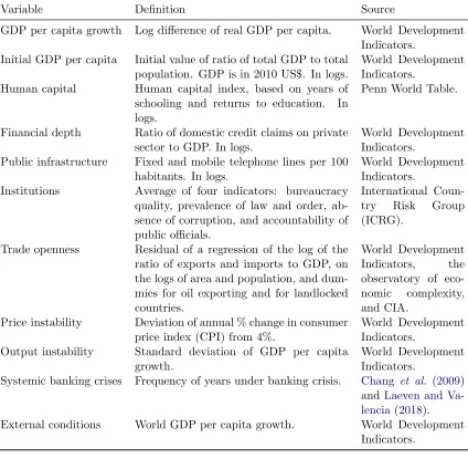
Our period of study spans from 1970 to 2015 for a sample of 80 countries. Table1shows constructions and definitions of the variables used in the estimation analysis, including the trade openness measure to be used.1

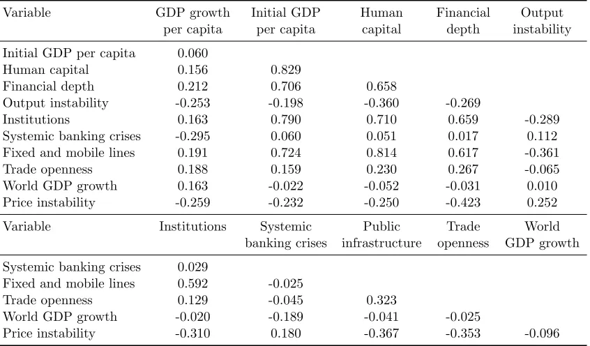
Summary statistics of the variables involved in the estimation analysis are given in Table2, and Table3shows pairwise correlations among the variables included in the estimation analysis; the initial GDP per capita is highly correlated with the structural variables and institution, which reveals that richer countries show better fundamentals.

2.4

Threshold regression model

Threshold regression models divide individual observations into classes based on the value of an observed variable, and have been widely used in time series analysis. Hansen

(1999) extends these models to a balanced panel data context –mainly by introducing econometric techniques using least squares (LS) estimation methods. As the growth models are dynamic, we use the econometric techniques developed byRam´ırez-Rond´an

(2015), who proposes maximum likelihood (ML) estimation for a dynamic panel thresh-old model using a first difference transformation. In this context, the first GDP per capita of each quinquennium represents the transitional dynamics.

We divide the observations into two regimes depending on whether the threshold variable qit is smaller or larger than the threshold parameter γ. The regimes are

distinguished by differing regression slopes, β1 and β2. For the identification of these

coefficients, the elements of qit−1 must not be time-invariant. The errorǫit is assumed

to be independent and identically distributed (iid) with mean zero and finite variance.

1

(9)

[image:9.612.81.505.80.495.2]

Table 1: Variables

Variable Definition Source

GDP per capita growth Log difference of real GDP per capita. World Development Indicators.

Initial GDP per capita Initial value of ratio of total GDP to total population. GDP is in 2010 US$. In logs.

World Development Indicators.

Human capital Human capital index, based on years of schooling and returns to education. In logs.

Penn World Table.

Financial depth Ratio of domestic credit claims on private sector to GDP. In logs.

Public infrastructure Fixed and mobile telephone lines per 100 habitants. In logs.

Institutions Average of four indicators: bureaucracy quality, prevalence of law and order, ab-sence of corruption, and accountability of public officials.

International Coun-try Risk Group (ICRG).

Trade openness Residual of a regression of the log of the ratio of exports and imports to GDP, on the logs of area and population, and dum-mies for oil exporting and for landlocked countries.

World Development Indicators, the observatory of eco-nomic complexity, and CIA.

Price instability Deviation of annual % change in consumer price index (CPI) from 4%.

Output instability Standard deviation of GDP per capita growth.

Systemic banking crises Frequency of years under banking crisis. Chang et al. (2009) andLaeven and Va-lencia(2018). External conditions World GDP per capita growth. World Development

Indicators.

The static and dynamic estimations of model (2) involves three steps: estimation, inference and testing.

Threshold and slope estimations

In the static methodology, one can eliminate the country-specific effect by removing country-specific means. Let ∆yit ≡yit−yit−1,β′ = (β1, β2)′ and assuming for simplicity

that there are no control variables; thus, the within transformation of model (2) is

∆y+

it =κy

+

it−1 +β′x +

it−1(γ) +ǫ +

it, (3)

where we define ∆y+

it ≡ ∆yit −T−1PT_t=1∆yit, y +

it−1 = yit−1 −T−1PT_t₌₁yit−1, ǫ +

(10)

[image:10.612.105.480.77.248.2]

Table 2: Summary statistics

Variable Obs. Mean Std. Dev. Min Max Growth per capita growth (%) 720 1.858 2.692 -10.457 15.839 Initial GDP per capita, in logs 720 8.375 1.545 5.431 11.561 Human capital, in logs 720 0.715 0.341 0.009 1.314 Financial depth, in logs 720 3.439 0.922 -0.192 5.396 Output instability 720 2.918 2.367 0.074 21.621 Institutions 720 3.520 1.446 0.5 6.0 Systemic banking crises 720 0.080 0.204 0.0 1.0 Public infrastructure, in logs 720 2.243 2.242 -3.416 5.295 Trade openness, in logs 720 0.044 0.440 -1.410 1.504 External conditions (%) 720 1.528 0.490 0.606 2.081 Price instability, in logs 720 2.594 0.898 0.013 8.783

Table 3: Correlations

Variable GDP growth Initial GDP Human Financial Output per capita per capita capital depth instability Initial GDP per capita 0.060

Human capital 0.156 0.829

Financial depth 0.212 0.706 0.658

Output instability -0.253 -0.198 -0.360 -0.269

Institutions 0.163 0.790 0.710 0.659 -0.289 Systemic banking crises -0.295 0.060 0.051 0.017 0.112 Fixed and mobile lines 0.191 0.724 0.814 0.617 -0.361 Trade openness 0.188 0.159 0.230 0.267 -0.065 World GDP growth 0.163 -0.022 -0.052 -0.031 0.010 Price instability -0.259 -0.232 -0.250 -0.423 0.252 Variable Institutions Systemic Public Trade World

banking crises infrastructure openness GDP growth Systemic banking crises 0.029

Fixed and mobile lines 0.592 -0.025

Trade openness 0.129 -0.045 0.323

World GDP growth -0.020 -0.189 -0.041 -0.025

Price instability -0.310 0.180 -0.367 -0.353 -0.096

ǫit−T−1PT_t=1ǫit and

x+

it−1(γ)≡

xit−11(q_it ≤γ)− _T1 PT_t₌₁x_it₋11(q_it ≤γ)

xit−11(qit> γ)− _T1 PT_t=1xit−11(qit > γ) !

.

For any given γ, the slope coefficients κ and β can be estimated by ordinary least squares (LS), and then the regression residuals are

bǫ+

it(γ) = ∆y

+

it −bκy

+

it−1−βb(γ)′x +

[image:10.612.83.506.281.529.2]

(11)

and the sum of squared errors to be minimized is

S(γ) =

n X

i=1

T X

t=1

b

ǫ+

it(γ)

2

. (5)

The criterion function (5) is not smooth, so conventional gradient algorithms are not suitable for its minimization. Hansen (1999, 2000) recommends estimation of the threshold by using a grid search over the threshold variable space. That is, construct an evenly spaced grid on the empirical support of the threshold variableqit, and minimizes

the concentrated sum of squared errors (5). Finally, once _bγ is obtained, the slope coefficient estimate is βb=βb(_bγ); and note that βb(_bγ) = (βb1(bγ),βb2(bγ))′.

As regards the dynamic methodology, we cannot consider a fixed effects transfor-mation for the dynamic threshold model since it could introduce a correlation between the transformed regressors and the transformed error term in the model, thus leading to inconsistency of the slope parameter. This is addressed by taking a first difference transformation of model (2) to eliminate the individual specific effect. We then have:

yit−yit−1−(yit−1−yit−2) = κ(yit−1−yit−2) +β1(xit−11(qit−1 ≤γ)−

xit−21(qit−2 ≤γ)) +β2(xit−11(qit−1 > γ)−xit−21(qit−2 > γ)) +ǫit−ǫit−1. (6)

Let ∆2

yit≡yit−yit−1−(yit−1−yit−2), ∆yit−1 ≡yit−1−yit−2, ∆x∗_it₋1 ≡xit−11(qit−1 ≤

γ)₋xit−21(qit−2 ≤ γ), ∆x +

it−1 ≡ xit−11(qit−1 > γ)−xit−21(qit−2 > γ), and ∆ǫit ≡

ǫit−ǫit−1, then equation (6) becomes:

∆2

yit=κ∆yit−1+β1∆x∗_it₋1(γ) +β2∆x +

it−1(γ) + ∆ǫit. (7)

The ML estimation of the dynamic panel linear model depends on the initial con-dition, which is key to establishing the consistency of the estimates (see Hsiao et al.,

2002). Thus, by assuming that the process has started from a finite period in the past, such that the expected changes in the initial endowments are the same across all indi-viduals, that model specification in the first period is given by ∆2

yi1 =δ+vi1, wereδis

an auxiliary external parameter. Further, we assume exogeneity of xit−1,

homoscedas-ticity across regimes, and by construction,E(vi1|xi) = 0, where xi = (xi0, xi1, ..., xiT)′,

and Ev2

i1 =σ 2

v.

Let ∆2

yi = (∆2yi1,∆2yi2, ...,∆2yiT)′ and ∆ǫi = (vi1,∆ǫi2, ...,∆ǫiT)′, and also define

ω = σ2

v/σ

2

(12)

probability distribution function of ∆2

yi is equivalent to (in logarithm):

lnL(δ, β, κ, γ, σ2

ǫ, ω) = −

nT

2 ln(2π)−

n

2ln|Ω| − 1 2

n X

i=1

∆ǫ(δ, β, κ, γ)′_Ω−1

ǫ(δ, β, κ, γ), (8)

where Ω is defined in Hsiao et al. (2002). The criterion function (8) is well defined, and depends on a fixed number of parameters. Then, the ML estimators of bδ, βb,_bκ, _bγ,

b

σ2

ǫ and ωb are the values that maximize lnL(δ, β, κ, γ, σ

2

ǫ, ω).

Hence, the algorithm for estimation has the following procedure:2

(i) for a given value of γ on the grid of the threshold variable, the criterion (8) is smooth; so we can calculate bδ(γ), βb(γ), _bκ(γ), σ_b2

ǫ(γ) and bω(γ) by maximizing that function; (ii) by

plugging those previous estimates in (8), it only depends onγ; and since the function is not smooth in γ, we find _bγ on the grid of the threshold variable which yields the highest value of the likelihood function; and finally, we set βb1 =βb1(bγ) and βb2 =βb2(bγ).

Asymptotic confidence intervals

When there is a threshold effect (β1 6= β2), Hansen (2000) has shown that threshold

estimate, _bγ, is consistent for γ0 (the true value of γ) and that the asymptotic

distri-bution is non standard. Hansen (1999) argues that the best ways to form confidence intervals for the threshold is to form the no rejection region using the likelihood ratio statistic for test on _bγ. To test hypothesis H0: γ = γ0, the likelihood ratio test is to

reject for large values of LR(γ0) where

LR(γ) =n(T ₋1)S(γ)−S(bγ)

S(_bγ) , (9) where S(γ) is defined in (5) in the static methodology, while in the dynamic case

S(γ) =Pn_i=1∆ǫbi(γ)′Ω− 1

∆ǫ_bi(γ) is the minimum distance estimator, which converges in

distribution as n _{→ ∞} to a random variableξ with distribution function P(ξ _≤ z) = (1₋exp(₋z/2))2

.

Then, the asymptotic distribution of the likelihood ratio statistic is non-standard, yet free of nuisance parameters (Hansen, 2000). Since the asymptotic distribution is pivotal, we use it to form valid asymptotic confidence intervals. Furthermore, the distribution functionξ has the inverse

c(α) =₋2ln(1₋√1₋α), (10)

2

(13)

where αis the significance level. The “no-rejection region” of confidence level 1₋α is the set of values ofγ such thatLR(γ)_≤c(α). This is easiest to find by plottingLR(γ) against γ and drawing a flat line atc(α).

Test for existence of threshold effects

It is important to determinate whether the threshold effect is statistically significant. The hypothesis of no threshold effects in (2) can be represented by the linear constraint

H0 : β1 = β2. Under the null hypothesis, H0, the threshold γ is not identified, so

classical tests have non-standard distributions. Hansen(2000) suggested a bootstrap to simulate the asymptotic distribution of the likelihood ratio test for this kind of models, so that thep-values constructed from the bootstrap procedure are asymptotically valid. Under the null hypothesis of no threshold, the model (1) without control variables is

∆yit=µi+κyit−1+β1xit−1+ǫit, (11)

after the within and first difference transformations are made in order to eliminate µi,

we get

∆y+

it =κy

+

it−1+β1x +

it−1+ǫ +

it, (12)

and

∆2

yit =κ∆yit−1+β1∆xit−1 + ∆ǫit, (13)

where x+

it−1 ≡xit−1−T−1PT_t₌₁xit−1 and ∆xit−1 =xit−1 −xit−2. The parameterβ1 is

estimated by LS or ML, yielding estimatesβb1, residualsbǫit and letS0 =Pn_i₌₁PT_t₌₁bǫ +2

it

the sum of squared residuals and S0 = Pn_i=1∆bǫ′itΩ−

1

∆_bǫit the minimum distance

esti-mator of the linear model in the static and dynamic methodologies, respectively. The likelihood ratio test of H0 is based on

F =n(T ₋1)S0−S(bγ)

(14)

3

Estimation and inference results

3.1

Linear model results

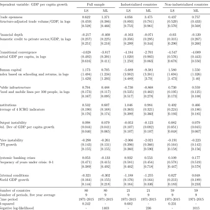
Table 4 provides the results of a linear model with two estimation methodologies. In the full sample, trade openness has a significant positive effect on growth under the maximum likelihood (ML) estimation, but not under the least squares (LS) estimation. Although the effect on economic growth seems to be inconclusive, when we split the sample into industrialized and non-industrialized countries we find that this positive and highly strong effect only occurs in industrialized countries, and that there are no effects in non-industrialized countries in either estimator.

As suggested by the theory, trade openness seems to have a differentiated effect on economic growth. We also find that financial development plays an enabling role on that effect –and indeed, we find that it consistently has a statistically significant effect on growth across estimators and samples. While there is no evidence that financial de-velopment has a direct effect on growth, it has an important indirect effect throughout trade openness.

3.2

Threshold effects

The first step is to test for the existence of a threshold effect in the relationship between GDP growth and trade openness using the F test of equation (14). This also involves estimating equation (2) and computing the residual sum of squares for the financial depth threshold. We conduct the test for the existence of threshold effects using a sample of 80 countries over nine five-year average periods between 1970 and 2015.3

The test for existence of threshold effects is shown in Table 5. The null hypothesis of no threshold effect against single threshold can be rejected at least at the 95 per cent significance level. The test statistics F for the single threshold are 23.057 and 18.711 with their corresponding bootstrapp-value of 0.005 and 0.042 for the static and dynamic methodologies, respectively. This indicates that the test for a single threshold is highly significant;4

thus, we conclude that there is strong evidence for threshold effects of financial depth in the trade and growth relationship.

3

These are the results when considering the full sample. The rejection of the null hypothesis also holds when considering other sub samples and different sets of control variables.

4

(15)

[image:15.612.81.509.76.503.2]

Table 4: Estimation results of the linear model

Dependent variable: GDP per capita growth Full sample Industrialized countries Non-industrialized countries

LS ML LS ML LS ML

Trade openness 0.622 1.371 4.056 3.475 0.437 0.757

Structure-adjusted trade volume/GDP, in logs (0.459) (0.386) (0.893) (0.781) (0.529) (0.433) [0.528] [0.466] [0.753] [0.961] [0.570] [0.568]

Financial depth -0.217 -0.460 -0.163 -0.071 -0.03 -0.120 Domestic credit to private sector/GDP, in logs (0.257) (0.225) (0.356) (0.295) (0.315) (0.267) [0.251] [0.216] [0.299] [0.344] [0.290] [0.260]

Transitional convergence -4.628 -3.817 -4.184 -2.701 -4.547 -4.009 Initial GDP per capita, in logs (0.492) (0.391) (1.020) (0.903) (0.576) (0.443) [0.616] [0.411] [1.250] [0.863] [0.678] [0.550]

Human capital 1.173 0.705 -5.689 -9.381 1.580 1.550

Index based on schooling and returns, in logs (1.494) (1.234) (3.982) (3.381) (1.694) (1.326) [1.429] [1.293] [4.489] [3.70] [1.473] [1.40]

Public infrastructure 0.704 0.488 -0.730 -0.868 0.730 0.559 Fixed and mobile lines per 100 people, in logs (0.173) (0.117) (0.535) (0.462) (0.195) (0.125)

[0.167] [0.095] [0.517] [0.278] [0.173] [0.108]

Institutions 0.532 0.607 1.046 0.984 0.402 0.466

Average of 4 ICRG indicators (0.190) (0.168) (0.363) (0.321) (0.224) (0.186) [0.176] [0.174] [0.399] [0.360] [0.193] [0.185]

Output instability 0.098 0.079 -0.053 -0.123 0.082 0.079 Std. Dev of GDP per capita growth (0.044) (0.041) (0.107) (0.082) (0.051) (0.045)

[0.046] [0.065] [0.107] [0.107] [0.048] [0.067]

Price instability -0.290 -0.261 -2.066 -2.021 -0.191 -0.223 CPI growth (0.143) (0.131) (0.396) (0.366) (0.164) (0.142) [0.155] [0.155] [0.360] [0.590] [0.158] [0.156]

Systemic banking crises 0.053 -0.133 0.932 0.553 0.109 0.177 Frequency of years under crisis: 0-1 (0.471) (0.415) (0.581) (0.454) (0.578) (0.519)

[0.389] [0.492] [0.402] [0.718] [0.447] [0.578]

External conditions -0.321 -0.302 -1.188 -1.255 0.027 0.048 World GDP growth (0.164) (0.155) (0.176) (0.164) (0.213) (0.189)

[0.144] [0.218] [0.164] [0.336] [0.183] [0.233]

Number of countries 80 80 21 21 59 59

Number of periods, five year average 9 9 9 9 9 9

Time period 1971-2015 1971-2015 1971-2015 1971-2015 1971-2015 1971-2015

R-squared 0.242 - 0.602 - 0.231

-Negative log-likelihood - 1403 - 236 - 1015

Notes: LS stands for (ordinary) least squares, and ML stands for maximum likelihood. Homoscedastic and heteroskedastic standard errors in parentheses and brackets, respectively.

3.3

Threshold estimate and its confidence interval

The second step is to compute the confidence intervals. The point estimate of the threshold and their asymptotic 90%, 95%, and 99% confidence intervals are reported in Table6. The two categories of countries and periods indicated by the point estimate are those with “low financial depth” and “high financial depth”. Moreover, the asymp-totic confidence intervals for the threshold are very tight, indicating low uncertainty regarding the nature of this division.

(16)

[image:16.612.115.472.79.207.2]

Table 5: Tests for threshold effects

Threshold Test Bootstrap Critical estimate (%) F p-value values Static methodology 27.429 23.057 0.005 13.7081/

15.6582/

21.3063/

Dynamic methodology 27.338 18.711 0.042 13.8021/

17.5572/

24.8163/

[image:16.612.70.510.270.336.2]

Note: 1/, 2/ and 3/ critical values at 10%, 5% and 1%, respectively. We used 1000 bootstrap replications for the test.

Table 6: Asymptotic confidence interval in threshold model

Threshold 90% confidence interval 95% confidence interval 99% confidence interval

Static

27.429 [26.306 ; 28.516] [26.193 ; 28.516] [25.939 ; 29.720] methodology

Dynamic

27.338 [26.183 ; 28.507] [25.924 ; 29.457] [22.925 ; 29.720] methodology

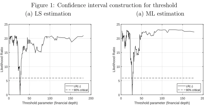
[image:16.612.88.487.435.640.2]

function is minimized at zero in the estimated threshold _bγ = 27.429 and _bγ = 27.338, corresponding to the static and dynamic methodologies with high precision and little uncertainty, since the confidence interval, the set of values below the dotted line, is very small.

Figure 1: Confidence interval construction for threshold (a) LS estimation (a) ML estimation

0 50 100 150 200

Threshold parameter (financial depth)

0 5 10 15 20 25

Likelihood Ratio

LR( ) 90% critical

0 50 100 150 200

Threshold parameter (financial depth)

0 5 10 15 20 25

Likelihood Ratio

(17)

3.4

Slope estimation results

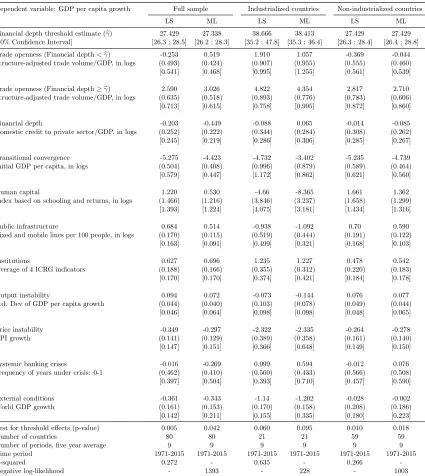
When considering a threshold model for the full sample (see Table7) the effect of trade openness on growth becomes differentiated between two regimes: countries with “low financial depth” –less than 27%– gain nothing from trade openness, while those with “high financial depth” benefit greatly from increased openness.5

Therefore, it can be concluded that there are two country regimes, and that trade openness has a different effect on growth for each according to financial depth level. The empirical literature supports these findings, as a poor level of financial development would not let domestic firms and economic sectors with scale economies to benefit from the potential lower costs and higher returns on capital, thus slowing development and growth. Conversely, greater financial depth level boosts economic growth.

To be sure, the marginal effect should not be the same for countries with different income levels and institutional quality. Table 7 also shows the results obtained for industrialized and non-industrialized countries.6

The results show that the estimated threshold around 38% domestic credit to the financial sector is considerably higher than that for non-industrialized countries (27%). But even though the level of financial development required for commercial openness to have a positive impact on growth is higher for industrialized countries, the marginal effect of trade on growth is also higher when the financial threshold is actually met: the elasticity for non-industrialized countries ranges from 2.7 to 2.8, while in industrialized countries it ranges from 4.4 to 4.8.

One might wonder whether the effect of openness when crossing the threshold in the case of industrialized countries is the same as in the case of non-industrialized countries; thus, we test the significance of the difference between the coefficients.7

The resulting range of the p-values of this test goes from 0.091 for the LS estimation to 0.095 for the ML estimation; the test favors the alternative hypothesis that the difference in the effects is statistically significant at a p-value less than 0.10. As to the null equality hypothesis of the thresholds of the industrialized and non-industrialized countries, we cannot apply an analogous test since the threshold parameter estimates do not converge to a normal distribution –but it might be expected that such estimates

5

Note that the null hypothesis of a linear model is rejected in all cases.

6

See AppendixAfor the classification based on United Nations.

7

As such coefficients come from different independent samples and regressions, we use the follow-ing Z test, followfollow-ing the approach of Clogg et al. (1995): Z = (βb2,Ind−βb2,N onind)/(SE(βb2,Ind)2+

SE(βb2,N onind))

0.5

, whereβb2,Indandβb2,N onindare the coefficients of trade openness once the threshold

(18)

[image:18.612.83.508.76.552.2]

Table 7: Estimation results of the threshold model

LS ML LS ML LS ML

Financial depth threshold estimate (bγ) 27.429 27.338 38.666 38.413 27.429 27.429 [90% Confidence Interval] [26.3 ; 28.5] [26.2 ; 28.3] [35.2 ; 47.8] [35.3 ; 46.4] [26.3 ; 28.4] [26.4 ; 28.8] Trade openness (Financial depth<bγ) -0.253 0.519 1.910 1.057 -0.369 -0.044 Structure-adjusted trade volume/GDP, in logs (0.493) (0.424) (0.907) (0.955) (0.555) (0.460) [0.541] [0.468] [0.995] [1.255] [0.561] [0.539]

Trade openness (Financial depth≥bγ) 2.590 3.026 4.822 4.354 2.817 2.710 Structure-adjusted trade volume/GDP, in logs (0.635) (0.518) (0.893) (0.776) (0.783) (0.606)

[0.713] [0.615] [0.758] [0.995] [0.872] [0.860]

Financial depth -0.203 -0.449 -0.088 0.065 -0.014 -0.085 Domestic credit to private sector/GDP, in logs (0.252) (0.222) (0.344) (0.284) (0.308) (0.262) [0.245] [0.219] [0.286] [0.306] [0.285] [0.267]

Transitional convergence -5.275 -4.423 -4.732 -3.402 -5.235 -4.739 Initial GDP per capita, in logs (0.504) (0.408) (0.996) (0.879) (0.589) (0.464) [0.579] [0.447] [1.172] [0.862] [0.621] [0.560]

Human capital 1.220 0.530 -4.66 -8.365 1.661 1.362

Index based on schooling and returns, in logs (1.466) (1.216) (3.846) (3.237) (1.658) (1.299) [1.393] [1.224] [4.075] [3.181] [1.434] [1.316]

[0.163] [0.091] [0.499] [0.321] [0.168] [0.103]

Institutions 0.627 0.696 1.235 1.227 0.478 0.542

[0.046] [0.064] [0.098] [0.098] [0.048] [0.065]

Price instability -0.349 -0.297 -2.322 -2.335 -0.264 -0.278 CPI growth (0.141) (0.129) (0.389) (0.358) (0.161) (0.140) [0.147] [0.151] [0.366] [0.648] [0.149] [0.150]

Systemic banking crises -0.016 -0.269 0.999 0.594 -0.012 0.076 Frequency of years under crisis: 0-1 (0.462) (0.410) (0.560) (0.433) (0.566) (0.508)

[0.397] [0.504] [0.393] [0.710] [0.457] [0.590]

External conditions -0.361 -0.343 -1.14 -1.202 -0.028 -0.002 World GDP growth (0.161) (0.153) (0.170) (0.158) (0.208) (0.186) [0.142] [0.211] [0.155] [0.335] [0.180] [0.223] Test for threshold effects (p-value) 0.005 0.042 0.060 0.095 0.010 0.018

Time period 1971-2015 1971-2015 1971-2015 1971-2015 1971-2015 1971-2015

R-squared 0.272 - 0.635 - 0.266

Notes: LS stands for (ordinary) least squares, and ML stands for maximum likelihood. Homoscedastic and heteroskedastic standard errors in parentheses and brackets, respectively. The test shows the probability value for the null hypothesis ofβb1=βb2. We used 1000 bootstrap

replications for the test.

are in fact different, since the confidence intervals of each do not overlap under any of the LS and ML estimations.

(19)

ex-port share of manufactured, high technology, and information and communication technology goods and services. Such sophisticated products –which include aerospace products, ICT goods and services, scientific products and instruments, and electrical machinery– have high capital, technology and R&D intensity.

Goods with a high level of sophistication require more technology and financial instruments to meet the needs of a more demanding industry; indeed, industrialized countries have better financial characteristics than non-industrialized ones in terms of financial institutions (depth, access, efficiency and stability) and financial markets (stock market capitalization, stock market turnover ratio, etc.). And industrialized countries are also associated with better developed infrastructure, higher human capital indexes, and higher quality institutions, making them well-suited to the production of technology-intensive goods.

3.5

Countries in each regime

The percentage of countries corresponding to low financial depth regime in the last quinquennium of the analysis is 30%, as shown in Table 8, indicating that with im-provements in their financial sector, these countries can take advantage of interna-tional specialization. It should be noted that the classifications of countries in Table

8are based on the dynamic methodology; the classifications with the static methodol-ogy estimates are the same, since the threshold estimates are rather similar for both methodologies.

Nevertheless, throughout the period of 1970-2015, the evolution in the level of fi-nancial development has not been the same across all countries: 31.3% remained in the regime of “high” financial depth, 20% stagnated in the “low” regime, and almost all the remaining countries enhanced their financial systems, with six exceptions –Algeria, Argentina, Cameroon, Cote d’Ivoire, Dominican Republic, and Venezuela– originally positioned in the “good” regime by their private credit levels, which have since de-creased to the extent that they have not been able to reach the required threshold level for the last 10 or 15 years at least.

These countries have been characterized by political instability, high export vulner-ability, dependence on oil exports, or even deep economic recessions. Thus, important preconditions for financial development to flourish –such as a robust institutional con-text or even trade openness, sufficient bureaucratic quality, and law and order– were absent (Chinn and Ito, 2006).

(20)

[image:20.612.76.513.78.365.2]

Table 8: Percentage of countries in each regime by quinquennium

Full sample

Regime 1971- 1976- 1981- 1986- 1991- 1996- 2001- 2006-

2011-1975 1980 1985 1990 1995 2000 2005 2010 2015

Financial depth<27.338% 57.5% 47.5% 41.3% 46.3% 55.0% 46.3% 43.8% 41.3% 30.0% Financial depth≥27.338% 42.5% 52.5% 58.8% 53.8% 45.0% 53.8% 56.3% 58.8% 70.0%

Industrialized countries

Regime 1971- 1976- 1981- 1986- 1991- 1996- 2001- 2006-

2011-1975 1980 1985 1990 1995 2000 2005 2010 2015

Non-industrialized countries

Regime 1971- 1976- 1981- 1986- 1991- 1996- 2001- 2006-

2011-1975 1980 1985 1990 1995 2000 2005 2010 2015

Non-industrialized countries under the industrialized threshold

Regime 1971- 1976- 1981- 1986- 1991- 1996- 2001- 2006-

2011-1975 1980 1985 1990 1995 2000 2005 2010 2015

countries, 40.7% of the countries still linger in the regime in which trade openness has a null marginal effect on economic growth (see Table 8). Furthermore, looking at the industrialized countries’ threshold for financial development, it can be seen that 60% of the countries do not comply with this requirement as of the last quinquennium in the sample.

3.6

Control variables results

Moving on to control variables, the initial GDP per capita was significant and negative as the neoclassic model predicts. Financial depth as a control variable is not significant, while institutions have a positive effect on GDP growth: a higher institutional quality of government increases GDP growth.8

Human capital has no additional statistically significant effect on economic growth, and public infrastructure, as measured by fixed and mobile telephones per 100 habitants, has a positive and statistically significant impact on growth.9

8

Similarly, Mauro(1995) finds that improving the control of corruption index in a standard devi-ation would make the annual growth rate rise by 1.3%.

9

(21)

Controls for stabilization policies in the estimation are output instability, price in-stability, and the frequency of systemic banking crises. Inflation has a negative and significant impact on GDP growth. This leads to the conclusion that higher macroe-conomic instability (approximated by the inflation rate) has a negative effect on the per capita GDP growth rate. Price instability negatively affected growth mainly in the 1980s, during which many countries recorded their highest levels of inflation. As a consequence, this period, characterized by high price instability leading to a reduced output growth rate, was known as “the lost decade”.

In the same way, the occurrence of banking crises may be detrimental to GDP growth. The indicator used states that a country is in crisis when significant signs of financial distress in the banking system (major bank runs, losses in the banking sys-tem, and/or bank liquidations); and if there are significant banking policy intervention measures in response to significant losses in the banking system (Laeven and Valencia,

2018), the effect on output growth is not significant. Similarly, the five-year average of output instability has no effect on long-term growth.

Finally, the world GDP growth variable as a control of external conditions in the estimation, incorporated as the five-year average of aggregate world GDP growth, has an overall negative impact on economies. The effects are higher in industrialized countries, while there are no effects in non-industrialized ones.

4

Robustness

4.1

Threshold location

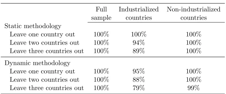
Even though the estimated threshold remains robust across methodologies in each subsample, we perform a sensitivity analysis of the threshold estimate; to this end, we estimate the threshold considering a leave-one-out, leave-two-out, and leave-three-out sample. We then analyze how many times these estimates fall within the 90% confidence interval of each sample estimation. This rules out the possibility of outliers in the sample, and evaluates the robustness of our estimates. The results of these tests indicate that the estimated threshold is robust to the changes in the sample, as none of the sub-sample estimates falls out of the confidence interval (see Table 9).

(22)

[image:22.612.108.476.93.246.2]

Table 9: Robustness of the threshold estimate

% of threshold estimates that fall in 90% confidence interval

Full Industrialized Non-industrialized sample countries countries Static methodology

Leave one country out 100% 100% 100% Leave two countries out 100% 94% 100% Leave three countries out 100% 89% 100%

Dynamic methodology

Leave one country out 100% 95% 100% Leave two countries out 100% 88% 100% Leave three countries out 100% 79% 99%

Note: for the leave two and three countries out tests, we used 200 draws from all possible combinations in each sample.

4.2

Additional control variables

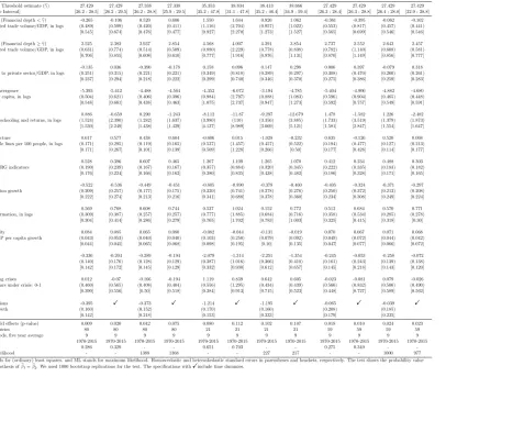
Several other control variables are considered in the empirical economic growth lit-erature; thus, in addition to the baseline specification in Table 10, we also employ the investment to GDP ratio and population growth as additional control variables. These variables also serve as a source of growth through capital and labor in a growth accounting exercise.

In regard to external conditions, the measurement variables used in the literature are international interest rates, international movement in capital flows, oil prices, commodity prices, global uncertainty, among others; in order to capture those external condition movements over the time period, we include time dummy variables instead of world GDP growth.

Table 7shows the results by including more control variables and, overall, the finan-cial depth threshold estimate and slope trade openness effects are quite robust. Finally, we include other country control variables like terrestrial precipitation, the Chinn-Ito index of financial openness (Chinn and Ito, 2006), and the debt to GDP ratio; but apart from reducing our availability of countries in the sample, such variables turn out to be non-significant in the regressions, so we decided not to include in the robustness exercise.

4.3

Comparison with other nonlinear models

(23)

[image:23.612.135.680.70.510.2]

Table 10: Estimation results with more control variables

LS ML LS ML LS ML

Financial depth Threshold estimate (bγ) 27.429 27.429 27.338 27.338 35.353 38.834 38.413 38.666 27.429 27.429 27.429 27.429 [90% Confidence Interval] [26.2 ; 28.5] [26.2 ; 29.5] [26.2 ; 28.8] [25.9 ; 29.5] [35.2 ; 47.8] [31.1 ; 47.8] [35.2 ; 46.4] [34.9 ; 59.4] [26.3 ; 28.4] [26.3 ; 28.8] [26.4 ; 28.8] [22.9 ; 28.8]

Trade openness (Financial depth<bγ) -0.265 -0.106 0.520 0.606 1.550 1.644 0.926 1.062 -0.361 -0.395 -0.062 -0.102 Structure-adjusted trade volume/GDP, in logs (0.489) (0.599) (0.420) (0.411) (1.116) (2.704) (0.957) (1.022) (0.553) (0.817) (0.457) (0.441)

[0.545] [0.674] [0.476] [0.477] [0.927] [2.270] [1.273] [1.527] [0.565] [0.699] [0.546] [0.546]

Trade openness (Financial depth≥bγ) 2.525 2.382 2.937 2.854 4.568 4.007 4.291 3.854 2.737 2.552 2.643 2.457 Structure-adjusted trade volume/GDP, in logs (0.631) (0.774) (0.514) (0.509) (0.880) (2.229) (0.778) (0.838) (0.782) (1.140) (0.608) (0.581)

[0.706] [0.855] [0.608] [0.610] [0.777] [1.916] [0.976] [1.131] [0.870] [1.149] [0.856] [0.777]

Financial depth -0.135 0.036 -0.390 -0.178 0.158 0.096 0.147 0.298 0.006 0.397 -0.079 0.318 Domestic credit to private sector/GDP, in logs (0.251) (0.315) (0.221) (0.221) (0.349) (0.818) (0.289) (0.297) (0.308) (0.470) (0.260) (0.261)

[0.237] [0.294] [0.218] [0.222] [0.299] [0.740] [0.346] [0.370] [0.275] [0.386] [0.259] [0.283]

Transitional convergence -5.393 -5.412 -4.488 -4.564 -4.352 -6.072 -3.194 -4.785 -5.404 -4.900 -4.882 -4.680 Initial GDP per capita, in logs (0.504) (0.621) (0.406) (0.396) (0.984) (2.797) (0.888) (1.083) (0.596) (0.904) (0.465) (0.448)

[0.548] [0.661] [0.438] [0.463] [1.075] [2.737] [0.947] [1.273] [0.592] [0.757] [0.549] [0.591]

Human capital 0.886 -0.659 0.290 -1.243 -8.112 -11.87 -9.297 -12.679 1.478 -1.582 1.226 -2.482 Index based on schooling and returns, in logs (1.524) (2.390) (1.282) (1.637) (3.980) (110) (3.356) (3.885) (1.733) (3.519) (1.379) (1.873)

[1.530] [2.249] [1.438] [1.429] [4.137] [8.989] [3.069] [5.121] [1.581] [2.847] [1.554] [1.647]

Public infrastructure 0.617 0.577 0.438 0.604 -0.606 0.015 -1.028 -0.232 0.635 -0.126 0.520 0.068 Fixed and mobile lines per 100 people, in logs (0.171) (0.295) (0.119) (0.165) (0.537) (1.457) (0.457) (0.522) (0.194) (0.477) (0.127) (0.213)

[0.171] [0.267] [0.101] [0.139] [0.509] [1.228] [0.266] [0.50] [0.177] [0.428] [0.114] [0.177]

Institutions 0.528 0.396 0.607 0.465 1.267 1.109 1.265 1.070 0.412 0.234 0.488 0.303 Average of 4 ICRG indicators (0.190) (0.239) (0.167) (0.167) (0.357) (0.884) (0.320) (0.345) (0.222) (0.335) (0.183) (0.182)

[0.176] [0.224] [0.166] [0.162] [0.380] [0.835] [0.438] [0.482] [0.186] [0.328] [0.171] [0.165]

Demographics -0.522 -0.536 -0.449 -0.451 -0.805 -0.890 -0.378 -0.460 -0.405 -0.324 -0.371 -0.297 Rate of population growth (0.209) (0.257) (0.177) (0.175) (0.320) (0.741) (0.278) (0.276) (0.250) (0.372) (0.213) (0.208)

[0.222] [0.274] [0.213] [0.216] [0.341] [0.688] [0.378] [0.360] [0.234] [0.308] [0.249] [0.224]

Investment 0.569 0.768 0.608 0.744 0.537 1.024 0.152 0.772 0.512 0.684 0.570 0.771 Gross capital formation, in logs (0.309) (0.387) (0.257) (0.257) (0.777) (1.885) (0.684) (0.716) (0.358) (0.534) (0.285) (0.278)

[0.304] [0.414] [0.286] [0.279] [0.765] [1.702] [0.783] [1.003] [0.325] [0.415] [0.318] [0.30]

Output instability 0.084 0.085 0.065 0.080 -0.082 -0.044 -0.131 -0.019 0.070 0.067 0.071 0.068 Std. Dev of GDP per capita growth (0.043) (0.053) (0.040) (0.040) (0.103) (0.250) (0.079) (0.092) (0.049) (0.072) (0.044) (0.042)

[0.044] [0.045] [0.065] [0.068] [0.098] [0.195] [0.10] [0.135] [0.047] [0.077] [0.066] [0.072]

Price instability -0.336 -0.204 -0.289 -0.194 -2.079 -1.314 -2.251 -1.354 -0.245 -0.053 -0.258 -0.072 CPI growth (0.140) (0.176) (0.128) (0.129) (0.387) (1.016) (0.366) (0.410) (0.161) (0.243) (0.139) (0.138)

[0.142] [0.172] [0.145] [0.129] [0.332] [0.930] [0.612] [0.657] [0.145] [0.218] [0.143] [0.120]

Systemic banking crises 0.012 -0.07 -0.166 -0.194 1.119 0.839 0.642 0.605 -0.023 -0.081 0.079 -0.026 Frequency of years under crisis: 0-1 (0.460) (0.565) (0.408) (0.404) (0.556) (1.295) (0.434) (0.439) (0.566) (0.832) (0.506) (0.490)

[0.390] [0.556] [0.50] [0.518] [0.384] [0.913] [0.715] [0.523] [0.448] [0.727] [0.589] [0.562]

External conditions -0.395 ✦ -0.373 ✦ -1.214 ✦ -1.195 ✦ -0.065 ✦ -0.039 ✦

World GDP growth (0.160) (0.152) (0.170) (0.160) (0.208) (0.185)

[0.142] [0.218] [0.153] [0.333] [0.179] [0.235]

Test for threshold effects (p-value) 0.009 0.020 0.042 0.075 0.080 0.112 0.102 0.107 0.018 0.010 0.024 0.023

Number of countries 80 80 80 80 21 21 21 21 59 59 59 59

Number of periods, five year average 9 9 9 9 9 9 9 9 9 9 9 9

Time period 1970-2015 1970-2015 1970-2015 1970-2015 1970-2015 1970-2015 1970-2015 1970-2015 1970-2015 1970-2015 1970-2015 1970-2015

R-squared 0.286 0.329 - - 0.651 0.703 - - 0.275 0.349 -

-Negative log-likelihood - - 1388 1368 - - 227 217 - - 1000 977

Notes: LS stands for (ordinary) least squares, and ML stands for maximum likelihood. Homoscedastic and heteroskedastic standard errors in parentheses and brackets, respectively. The test shows the probability value for the null hypothesis ofbβ1=βb2. We used 1000 bootstrap replications for the test. The specifications with✦include time dummies.

(24)

[image:24.612.83.501.175.613.2]

and Abida(2014). These results suggest that the effect of trade openness on growth is different for different values of financial depth, while the unique effect of trade openness is not significant. We can again see a differentiated marginal effect of trade openness on growth when we split the full sample into two sub samples (industrialized and non-industrialized countries).

Table 11: Estimation results of the interaction model

LS ML LS ML LS ML

Trade openness -1.635 -0.495 -2.390 -5.991 -1.850 -1.276 Structure-adjusted trade volume/GDP, in logs (1.008) (0.852) (3.096) (2.550) (1.166) (0.969)

[1.016] [0.799] [2.970] [3.688] [1.081] [0.992]

Trade openness*financial depth 0.787 0.625 1.465 2.159 0.839 0.717 (0.314) (0.255) (0.675) (0.556) (0.382) (0.306) [0.297] [0.226] [0.621] [0.798] [0.355] [0.325]

Financial depth -0.143 -0.414 -0.197 -0.091 0.066 -0.034 Domestic credit to private sector/GDP, in logs (0.257) (0.225) (0.351) (0.283) (0.317) (0.268)

[0.255] [0.220] [0.295] [0.317] [0.299] [0.268]

Transitional convergence -5.127 -4.208 -4.426 -3.252 -5.093 -4.506 Initial GDP per capita, in logs (0.528) (0.421) (1.010) (0.876) (0.625) (0.489)

[0.614] [0.442] [1.185] [0.696] [0.674] [0.581]

Human capital 1.305 0.638 -5.679 -8.661 1.737 1.499 Index based on schooling and returns, in logs (1.487) (1.228) (3.920) (3.244) (1.687) (1.318)

[1.401] [1.267] [4.494] [3.187] [1.444] [1.369]

[0.164] [0.094] [0.518] [0.312] [0.169] [0.108]

Institutions 0.609 0.673 1.132 1.106 0.470 0.524

[0.047] [0.065] [0.101] [0.095] [0.049] [0.067]

Price instability -0.326 -0.281 -2.210 -2.251 -0.224 -0.246 CPI growth (0.143) (0.130) (0.395) (0.356) (0.164) (0.142)

[0.154] [0.157] [0.364] [0.603] [0.156] [0.157]

Systemic banking crises 0.006 -0.213 1.047 0.649 0.014 0.102 Frequency of years under crisis: 0-1 (0.468) (0.414) (0.575) (0.435) (0.577) (0.517)

[0.392] [0.501] [0.411] [0.704] [0.451] [0.582]

External conditions -0.318 -0.304 -1.216 -1.285 0.033 0.050 World GDP growth (0.163) (0.154) (0.173) (0.158) (0.211) (0.188)

[0.143] [0.217] [0.162] [0.347] [0.182] [0.231]

Time period 1971-2015 1971-2015 1971-2015 1971-2015 1971-2015 1971-2015

R-squared 0.252 - 0.618 - 0.241

Notes: LS stands for (ordinary) least squares, and ML stands for maximum likelihood. Homoscedastic and heteroskedastic standard errors in parentheses and brackets, respectively.

(25)

ad-dition, both the R-squared and the negative log-likelihood favor the threshold model against the interaction model; that is, the threshold model fits the data better than the interaction model in the full, industrialized, and non-industrialized samples.

5

Conclusion

In this paper, we examine the implications of financial sector development for the trade openness and growth nexus. We find that financial sector development, from a clearly identifiable threshold, is a key enabler of the growth benefits of trade. This finding is consistent with the recent literature suggesting that the indirect effects of financial development on growth might be as strong as the direct effects, and that these effects are concentrated on trade. We find that these results are robust to changes in specification and to the sequential elimination of three countries from the sample at a time. This finding provides evidence that financial sector development is itself a source of comparative advantage. The use of a dynamic panel regression is justified as it allows us to clearly identify the financial sector development threshold within a tractable framework.

We also find that the financial-sector-threshold enablers of growth benefits from trade are greater for industrialized than for non-industrialized economies. This is consistent with the literature’s conjecture that countries that export more capital-intensive and finance-dependent sectors need deeper financial sectors. Importantly, the financial development thresholds we estimate are much lower than the 80-100 percent of GDP thresholds found to be detrimental to economic growth elsewhere in the literature. Furthermore, industrialized economies also gain considerably more once their threshold is met.

(26)

References

Aghion, P., P. Bacchetta, R. Ranciere and K. Rogoff (2009). “Exchange rate volatility and productivity growth: The role of financial development.” Journal of Monetary Economics, 56(4), 494-513.

Arcand, J., E. Berkes and U. Panizza (2015). “Too much finance?” Journal of Eco-nomic Growth, 20(2), 105-148.

Beck, T. (2002). “Financial development and international trade: is there a link?”

Journal of International Economics, 57(1), 107-131.

Blyde, J. and E. Fern´andez-Arias (2005) “Why Latin America is falling behind.” In: Manuelli, R., J. Blyde and E. Fern´andez-Arias (eds.), Sources of growth in Latin America: what is missing?. Washington D.C.: Inter-American Development Bank.

Buera, F., J. Kaoshki and Y. Shin (2011). “Finance and development: a tale of two sectors.”American Economic Review, 101(5), 1964-2002.

Chaney, T. (2016). “Liquidity constrained exporters.” Journal of Economic Dynamics and Control, 72(C), 141-154.

Chang, R., L. Kaltani and N. Loayza (2009). “Openness can be good for growth: the role of policy complementarities.”Journal of Development Economics, 90(1), 33-49.

Chinn, M. and H. Ito (2006). “What matters for financial development? Capital con-trols, institutions, and interactions.”Journal of Development Economics, 81(1), 163-192.

Clogg, C., E. Petkova and A. Haritou (1995). “Statistical methods for comparing regres-sion coefficients between models.”American Journal of Sociology, 100(5), 1261-1293.

Dollar, D. (1992). “Outward-oriented developing economies really grow more rapidly: evidence from 95 LDCs, 1976-85.” Economic Development and Cultural Change, 40(3), 523-544.

Edwards, S. (1998). “Openness, productivity, and growth: what do we really know?”

Economic Journal, 108(447), 383-398.

(27)

Frankel, A. and D. Romer (1999). “Does trade cause growth?” American Economic Review, 89(3), 379-399.

Grossman, G. and E. Helpman (1991). Innovation and growth in the global economy.

Cambridge, Mass.: MIT Press.

Hansen, B. (1999). “Threshold effects in non-dynamic panels: estimation, testing and inference.” Journal of Econometrics, 93(2), 345-368.

Hansen, B. (2000). “Sample splitting and threshold estimation.”Econometrica, 68(2), 575-603.

Hausmann, R., J. Hwang and D. Rodrik (2007). “What you export matters”. Journal of Economic Growth, 12(1), 1-25.

Hsiao, C., M. Pesaran and K. Tahmiscioglu (2002). “Maximum likelihood estimation of fixed effects dynamic panel data models covering short time periods.” Journal of Econometrics, 109(1), 107-150.

Jones, C. and P. Romer (2010). “The new Kaldor facts: ideas, institutions, population, and human capital.”American Economic Journal: Macroeconomics, 2(1), 224-245.

Kim, D., S. Lin and Y. Suen (2010). “Are financial development and trade openness complements or substitutes?” Southern Economic Journal, 76(3), 827-845.

Kletzer, K. and P. Bardhan (1987). “Credit markets and patterns of international trade.”Journal of Development Economics 27(1-2), 57-70.

Kohn, D., F. Leibovici and M. Szkup (2017). “Financial frictions, trade, and misallo-cation.” CAF - Working paper, 2017/19.

Laeven, L. and F. Valencia (2018). “Systemic banking crises revisited.” IMF Working Paper 18/206.

Lee, H., L. Ricci and R. Rigobon (2004). “Once again, is openness good for growth?”

Journal of Development Economics, 75(2), 451-472.

Leibovici, F. (2018). “Financial development and international trade.” Working Paper 15, Federal Reserve Bank of St. Louis.

(28)

Loayza, N., P. Fajnzylber and C. Calder´on (2005).Economic growth in Latin America and the Caribbean. Stylized Facts, explanations and forecasts. World Bank Publica-tions 7315, The World Bank.

Matsuyama, K. (1992). “Agricultural productivity, comparative advantage, and eco-nomic growth.”Journal of Economic Theory, 58(2), 317-334.

Mauro, P. (1995). “Corruption and growth.” Quarterly Journal of Economics, 110(3), 681-712.

McKinnon, R. (1973). “Money and capital in economic development.” Washington D.C.: Brookings Institution.

Levine, R., N. Loayza and T. Beck (2000). “Financial intermediation and growth: Causality and causes.”Journal of Monetary Economics, 46(1), 31-77.

Nunn, N. and D. Trefler (2014). “Domestic institutions as a source of comparative advantage.” In: Gopinath, G., E. Helpman and K. Rogoff (eds.), Handbook of In-ternational Economics, 263-315.

Pritchett, L. (1996). “Measuring outward orientation in LDCs: can it be done?” Jour-nal of Development Economics, 49(2), 307-335.

Ram´ırez-Rond´an, N. (2015). “Maximum likelihood estimation of dynamic panel thresh-old models.” Peruvian Economic Association Working Paper 32.

Rajan, R. and L. Zingales (1998). “Financial dependence and growth.”American Eco-nomic Review, 88(3), 559-586.

Rodr´ıguez, F. (2007). “Openness and growth: what have we learned?” DESA Working Paper 51.

Rodr´ıguez, F. and D. Rodrik (2001). “Trade policy and economic growth: a skeptics guide to the cross-national evidence.” in Bernanke, B. and K. Rogoff (eds.), NBER

Macroeconomics Annual 2000, 15, MIT Press, 261-325.

Rousseau, P. and P. Wachtel (2011). “What is happening to the impact of financial deepening on economic growth?” Economic Inquiry, 49(1), 276-288.

(29)

Ula¸san, B. (2015). “Trade openness and economic growth: panel evidence.” Applied Economics Letters, 22(2), 163-167.

Wacziarg, R. and K. Welch (2008). “Trade liberalization and growth: new evidence.”

World Bank Economic Review, 22(2), 187-231.

Young, A. (1991). “Learning by doing and the dynamic effects of international trade.”

Quarterly Journal of Economics, 106(2), 369-405.

Zghidi, N. and Z. Abida (2014). “Financial development, trade openness and economic growth in North African countries.” The Romanian Economic Journal, 17(53), 91-120.

[image:29.612.85.502.347.624.2]

A