Learning Word Meta-Embeddings
Wenpeng YinandHinrich Sch¨utze
Center for Information and Language Processing LMU Munich, Germany
Abstract
Word embeddings – distributed represen-tations of words – in deep learning are beneficial for many tasks in NLP. How-ever, different embedding sets vary greatly in quality and characteristics of the cap-tured information. Instead of relying on a more advanced algorithm for embed-ding learning, this paper proposes an en-semble approach of combining different public embedding sets with the aim of learning metaembeddings. Experiments on word similarity and analogy tasks and on part-of-speech tagging show better per-formance of metaembeddings compared to individual embedding sets. One advan-tage of metaembeddings is the increased vocabulary coverage. We release our metaembeddings publicly at http:// cistern.cis.lmu.de/meta-emb.
1 Introduction
Recently, deep neural network (NN) models have achieved remarkable results in NLP (Collobert and Weston, 2008; Sutskever et al., 2014; Yin and Sch¨utze, 2015). One reason for these results are word embeddings, compact distributed word representations learned in an unsupervised manner from large corpora (Bengio et al., 2003; Mnih and Hinton, 2009; Mikolov et al., 2013a; Pennington et al., 2014).
Some prior work has studied differences in per-formance of different embedding sets. For exam-ple, Chen et al. (2013) show that the embedding sets HLBL (Mnih and Hinton, 2009), SENNA (Collobert and Weston, 2008), Turian (Turian et al., 2010) and Huang (Huang et al., 2012) have great variance in quality and characteristics of the semantics captured. Hill et al. (2014; 2015a) show
that embeddings learned by NN machine transla-tion models can outperform three representative monolingual embedding sets: word2vec (Mikolov et al., 2013b), GloVe (Pennington et al., 2014) and CW (Collobert and Weston, 2008). Bansal et al. (2014) find that Brown clustering, SENNA, CW, Huang and word2vec yield significant gains for dependency parsing. Moreover, using these repre-sentations together achieved the best results, sug-gesting their complementarity. These prior stud-ies motivate us to explore an ensemble approach. Each embedding set is trained by a different NN on a different corpus, hence can be treated as a distinct description of words. We want to lever-age thisdiversityto learn better-performing word embeddings. Our expectation is that the ensemble contains more information than each component embedding set.
The ensemble approach has two benefits. First,
enhancement of the representations: metadings perform better than the individual embed-ding sets. Second, coverage: metaembeddings cover more words than the individual embedding sets. The first three ensemble methods we intro-duce are CONC, SVD and 1TON and they directly only have the benefit of enhancement. They learn metaembeddings on the overlapping vocabulary of the embedding sets. CONC concatenates the vec-tors of a word from the different embedding sets. SVD performs dimension reduction on this con-catenation. 1TON assumes that a metaembedding for the word exists, e.g., it can be a randomly initialized vector in the beginning, and uses this metaembedding to predict representations of the word in the individual embedding sets by projec-tions – the resulting fine-tuned metaembedding is expected to contain knowledge from all individual embedding sets.
To also address the objective of increased cov-erage of the vocabulary, we introduce 1TON+,
a modification of 1TON that learns metaembed-dings for all words in thevocabulary unionin one step. Let an out-of-vocabulary (OOV) word w of embedding set ES be a word that is not cov-ered by ES (i.e., ES does not contain an embed-ding forw).1 1TON+first randomly initializes the embeddings for OOVs and the metaembeddings, then uses a prediction setup similar to 1TON to update metaembeddings as well as OOV embed-dings. Thus, 1TON+simultaneously achieves two goals: learning metaembeddings and extending the vocabulary (for both metaembeddings and in-vidual embedding sets).
An alternative method that increases cover-age is MUTUALLEARNING. MUTUALLEARNING learns the embedding for a word that is an OOV in embedding set from its embeddings in other em-bedding sets. We will use MUTUALLEARNING to increase coverage for CONC, SVD and 1TON, so that these three methods (when used together with MUTUALLEARNING) have the advantages of both performance enhancement and increased coverage.
In summary, metaembeddings have two benefits compared to individual embedding sets: enhance-ment of performance and improved coverage of the vocabulary. Below, we demonstrate this ex-perimentally for three tasks: word similarity, word analogy and POS tagging.
If we simply view metaembeddings as a way of coming up with better embeddings, then the alter-native is to develop a single embedding learning algorithm that produces better embeddings. Some improvements proposed before have the disadvan-tage of increasing the training time of embedding learning substantially; e.g., the NNLM presented in (Bengio et al., 2003) is an order of magnitude less efficient than an algorithm like word2vec and, more generally, replacing a linear objective func-tion with a nonlinear objective funcfunc-tion increases training time. Similarly, fine-tuning the hyperpa-rameters of the embedding learning algorithm is complex and time consuming. In terms of cover-age, one might argue that we can retrain an ex-isting algorithm like word2vec on a bigger cor-pus. However, that needs much longer training time than our simple ensemble approaches which achieve coverage as well as enhancement with less effort. In many cases, it is not possible to retrain
1We do not consider words in this paper that are not
cov-ered by any of the individual embedding sets. OOV refers to a word that is covered by a proper subset of ESs.
using a different algorithm because the corpus is not publicly available. But even if these obsta-cles could be overcome, it is unlikely that there ever will be a single “best” embedding learn-ing algorithm. So the current situation of multi-ple embedding sets with different properties be-ing available is likely to persist for the forseeable future. Metaembedding learning is a simple and efficient way of taking advantage of this diver-sity. As we will show below they combine several complementary embedding sets and the resulting metaembeddings are stronger than each individual set.
2 Related Work
Related work has focused on improving perfor-mance on specific tasks by using several embed-ding sets simultaneously. To our knowledge, there is no work that aims to learn generally useful metaembeddings from individual embedding sets. Tsuboi (2014) incorporates word2vec and GloVe embeddings into a POS tagging system and finds that using these two embedding sets together is better than using them individually. Similarly, Turian et al. (2010) find that using Brown clus-ters, CW embeddings and HLBL embeddings for Name Entity Recognition and chunking tasks to-gether gives better performance than using these representations individually.
Luo et al. (2014) adapt CBOW (Mikolov et al., 2013a) to train word embeddings on differ-ent datasets – a Wikipedia corpus, search click-through data and user query data – for web search ranking and for word similarity. They show that using these embeddings together gives stronger re-sults than using them individually.
Both (Yin and Sch¨utze, 2015) and (Zhang et al., 2016) try to incorporate multiple embedding sets into channels of convolutional neural network system for sentence classification tasks. The bet-ter performance also hints the complementarity of component embedding sets, however, such kind of incorporation brings large numbers of training pa-rameters.
Vocab Size Dim Training Data
HLBL (Mnih and Hinton, 2009) 246,122 100 Reuters English newswire August 1996-August 1997 Huang (Huang et al., 2012) 100,232 50 April 2010 snapshot of Wikipedia Glove (Pennington et al., 2014) 1,193,514 300 42 billion tokens of web data, from Common Crawl CW (Collobert and Weston, 2008) 268,810 200 Reuters English newswire August 1996-August 1997 word2vec (Mikolov et al., 2013b) 929,022 300 About 100 billion tokens from Google News
Table 1: Embedding Sets (Dim: dimensionality of word embeddings).
Sch¨utze, 2015; Zhang et al., 2016). In our work, we can leverage any publicly available embed-ding set learned by any learning algorithm. Our metaembeddings (i) do not require access to re-sources such as large computing infrastructures or proprietary corpora; (ii) are derived by fast and simple ensemble learning from existing embed-ding sets; and (iii) have much lower dimensional-ity than a simple concatentation, greatly reducing the number of parameters in any system that uses them.
An alternative to learning metaembeddings from embeddings is the MVLSA method that learns powerful embeddings directly from multi-ple data sources (Rastogi et al., 2015). Rastogi et al. (2015) combine a large number of data sources and also run two experiments on the embedding sets Glove and word2vec. In contrast, our fo-cus is on metaembeddings, i.e., embeddings that are exclusively based on embeddings. The ad-vantages of metaembeddings are that they outper-form individual embeddings in our experiments, that few computational resources are needed, that no access to the original data is required and that embeddings learned by new powerful (includ-ing nonlinear) embedd(includ-ing learn(includ-ing algorithms in the future can be immediately taken advantage of without any changes being necessary to our basic framework. In future work, we hope to compare MVLSA and metaembeddings in effectiveness (Is using the original corpus better than using embed-dings in some cases?) and efficiency (Is using SGD or SVD more efficient and in what circum-stances?).
3 Experimental Embedding Sets
In this work, we use five released embedding sets.
(i) HLBL. Hierarchical log-bilinear (Mnih and
Hinton, 2009) embeddings released by Turian et al. (2010);2 246,122 word embeddings, 100
di-mensions; training corpus: RCV1 corpus (Reuters English newswire, August 1996 – August 1997).
2metaoptimize.com/projects/wordreprs
(ii) Huang.3 Huang et al. (2012) incorporate
global context to deal with challenges raised by words with multiple meanings; 100,232 word em-beddings, 50 dimensions; training corpus: April 2010 snapshot of Wikipedia. (iii) GloVe4
(Pen-nington et al., 2014). 1,193,514 word embed-dings, 300 dimensions; training corpus: 42 billion tokens of web data, from Common Crawl. (iv)
CW (Collobert and Weston, 2008). Released by Turian et al. (2010);5 268,810 word embeddings,
200 dimensions; training corpus: same as HLBL.
(v) word2vec (Mikolov et al., 2013b) CBOW;6
929,022 word embeddings (we discard phrase embeddings), 300 dimensions; training corpus: Google News (about 100 billion words). Table 1 gives a summary of the five embedding sets.
The intersection of the five vocabularies has size 35,965, the union has size 2,788,636.
4 Ensemble Methods
This section introduces the four ensemble meth-ods: CONC, SVD, 1TON and 1TON+.
4.1 CONC: Concatenation
In CONC, the metaembedding of w is the con-catenation of five embeddings, one each from the five embedding sets. For GloVe, we perform L2 normalization for each dimension across the vo-cabulary as recommended by the GloVe authors. Then each embedding of each embedding set is L2-normalized. This ensures that each embedding set contributes equally (a value between -1 and 1) when we compute similarity via dot product.
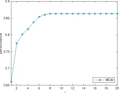
We would like to make use of prior knowl-edge and give more weight to well performing em-bedding sets. In this work, we give GloVe and word2vec weighti > 1and weight 1 to the other three embedding sets. We use MC30 (Miller and Charles, 1991) as dev set, since all embedding sets fully cover it. We seti= 8, the value in Figure 1
3ai.stanford.edu/˜ehhuang
where performance reaches a plateau. After L2 normalization, GloVe and word2vec embeddings are multiplied byiand remaining embedding sets are left unchanged.
The dimensionality of CONC metaembeddings
isk= 100+50+300+200+300 = 950. We also
tried equal weighting, but the results were much worse, hence we skip reporting it. It nevertheless gives us insight that simple concatenation, without studying the difference among embedding sets, is unlikely to achieve enhancement. The main disad-vantage of simple concatenation is that word em-beddings are commonly used to initialize words in DNN systems; thus, the high-dimensionality of concatenated embeddings causes a great increase in training parameters.
4.2 SVD: Singular Value Decomposition
We do SVD on above weighted concatenation vec-tors of dimensionk= 950.
Given a set of CONC representations for n words, each of dimensionality k, we compute an SVD decomposition C = USVT of the
corre-spondingn×kmatrixC. We then useUd, the first
ddimensions ofU, as the SVD metaembeddings of the n words. We apply L2-normalization to embeddings; similarities of SVD vectors are com-puted as dot products.
d denotes the dimensionality of metaembed-dings in SVD, 1TON and 1TON+. We use d =
200throughout and investigate the impact ofd be-low.
[image:4.595.310.524.127.190.2]4.3 1TON
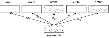
Figure 2 depicts the simple neural network we em-ploy to learn metaembeddings in 1TON. White
i
2 4 6 8 10 12 14 16 18 20
performance
0.65 0.7 0.75 0.8 0.85 0.9
MC30
Figure 1: Performance vs. Weight scalari
rectangles denote known embeddings. The target to learn is the metaembedding (shown as shaded rectangle). Metaembeddings are initialized ran-domly.
Figure 2: 1toN
Let c be the number of embedding sets under consideration, V1, V2, . . . , Vi, . . . , Vc their
vocab-ularies and V∩ = ∩c
i=1Vi the intersection, used
as training set. LetV∗ denote the metaembedding space. We define a projectionf∗ifrom spaceV∗to spaceVi(i= 1,2, . . . , c) as follows:
ˆ
wi =M∗iw∗ (1) whereM∗i ∈Rdi×d,w∗ ∈Rdis the metaembed-ding of wordwin space V∗ andwˆi ∈ Rdi is the
projected (or learned) representation of wordwin spaceVi. The training objective is as follows:
E =Xc i=1
ki·( X
w∈V∩
|wˆi−wi|2+l2· |M∗i|2) (2)
In Equation 2,kiis the weight scalar of theith
em-bedding set, determined in Section 4.1, i.e,ki = 8
for GloVe and word2vec embedding sets, other-wiseki= 1;l2is the weight of L2 normalization. The principle of 1TON is that we treat each in-dividual embedding as a projection of the metaem-bedding, similar to principal component analysis. An embedding is a description of the word based on the corpus and the model that were used to cre-ate it. The metaembedding tries to recover a more comprehensive description of the word when it is trained to predict the individual descriptions.
[image:4.595.83.280.577.731.2]4.4 1TON+
Recall that an OOV (with respect to embedding set ES) is defined as a word unknown in ES. 1TON+ is an extension of 1TON that learns embeddings for OOVs; thus, it does not have the limitation that it can only be run on overlapping vocabulary.
[image:5.595.310.524.63.107.2]Figure 3: 1toN+
Figure 3 depicts 1TON+. In contrast to Figure 2, we assume that the current word is an OOV in embedding sets 3 and 5. Hence, in the new learn-ing task, embeddlearn-ings 1, 2, 4 are known, and em-beddings 3 and 5 and the metaembedding are tar-gets to learn.
We initialize all OOV representations and metaembeddings randomly and use the same map-ping formula as for 1TON to connect a metaem-bedding with the individual emmetaem-beddings. Both metaembedding and initialized OOV embeddings are updated during training.
Each embedding set contains information about only a part of the overall vocabulary. However, it can predict what the remaining part should look like by comparing words it knows with the infor-mation other embedding sets provide about these words. Thus, 1TON+ learns a model of the de-pendencies between the individual embedding sets and can use these dependencies to infer what the embedding of an OOV should look like.
CONC, SVD and 1TON compute metaembed-dings only for the intersection vocabulary. 1TON+ computes metaembeddings for the union of all in-dividual vocabularies, thus greatly increasing the coverage of individual embedding sets.
5 MUTUALLEARNING
MUTUALLEARNING is a method that extends CONC, SVD and 1TON such that they have in-creased coverage of the vocabulary. With MU -TUALLEARNING, all four ensemble methods – CONC, SVD, 1TON and 1TON+– have the ben-efits of both performance enhancement and in-creased coverage and we can use criteria like per-formance, compactness and efficiency of training
bs lr l2
1TON 200 0.005 5×10⁻⁴
[image:5.595.78.285.161.233.2]MUTUALLEARNING(ml) 200 0.01 5×10⁻⁸ 1TON+ 2000 0.005 5×10⁻⁴
Table 2: Hyperparameters. bs: batch size; lr: learning rate;l2: L2 weight.
to select the best ensemble method for a particular application.
MUTUALLEARNING is applied to learn OOV embeddings for all c embedding sets; however, for ease of exposition, let us assume we want to compute embeddings for OOVs for embedding set j only, based on known embeddings in the other c−1embedding sets, with indexesi∈ {1. . . j−
1, j+ 1. . . c}. We do this by learningc−1 map-pings fij, each a projection from embedding set
Eito embedding setEj.
Similar to Section 4.3, we train mapping fij
on the intersection Vi ∩ Vj of the vocabularies
covered by the two embedding sets. Formally,
ˆ
wj = fij(wi) = Mijwi whereMij ∈ Rdj×di,
wi ∈ Rdi denotes the representation of word w
in space Vi and wˆj is the projected
metaembed-ding of wordwin spaceVj. Training loss has the
same form as Equation 2 except that there is no “Pci=1ki” term. A total ofc−1projectionsfij
are trained to learn OOV embeddings for embed-ding setj.
Letwbe a word unknown in the vocabularyVj
of embedding setj, but known inV1, V2, . . . , Vk.
To compute an embedding for w in Vj, we first
compute thekprojectionsf1j(w1),f2j(w2),. . ., fkj(wk)from the source spacesV1, V2, . . . , Vk to
the target spaceVj. Then, the element-wise
aver-age off1j(w1), f2j(w2), . . ., fkj(wk) is treated
as the representation ofwinVj. Our motivation is
that – assuming there is a true representation ofw inVj and assuming the projections were learned
well – we would expect all the projected vectors to be close to the true representation. Also, each source space contributes potentially complemen-tary information. Hence averaging them is a bal-ance of knowledge from all source spaces.
6 Experiments
We train NNs by back-propagation with AdaGrad (Duchi et al., 2011) and mini-batches. Table 2 gives hyperparameters.
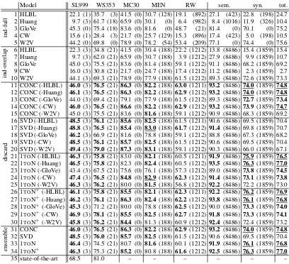
Model SL999 WS353 MC30 MEN RW sem. syn. tot.
ind-full
1 HLBL 22.1 (1) 35.7 (3) 41.5 (0) 30.7 (128) 19.1 (892) 27.1 (423) 22.8 (198) 24.7 2 Huang 9.7 (3) 61.7 (18) 65.9 (0) 30.1 (0) 6.4 (982) 8.4 (1016) 11.9 (326) 10.4 3 GloVe 45.3 (0) 75.4 (18) 83.6 (0) 81.6 (0) 48.7 (21) 81.4 (0) 70.1 (0) 75.2 4 CW 15.6 (1) 28.4 (3) 21.7 (0) 25.7 (129) 15.3 (896) 17.4 (423) 5.0 (198) 10.5 5 W2V 44.2 (0) 69.8 (0) 78.9 (0) 78.2 (54) 53.4 (209) 77.1 (0) 74.4 (0) 75.6
ind-o
verlap
6 HLBL 22.3 (3) 34.8 (21) 41.5 (0) 30.4 (188) 22.2 (1212) 13.8 (8486) 15.4 (1859) 15.4 7 Huang 9.7 (3) 62.0 (21) 65.9 (0) 30.7 (188) 3.9 (1212) 27.9 (8486) 9.9 (1859) 10.7 8 GloVe 45.0 (3) 75.5 (21) 83.6 (0) 81.4 (188) 59.1 (1212) 91.1 (8486) 68.2 (1859) 69.2 9 CW 16.0 (3) 30.8 (21) 21.7 (0) 24.7 (188) 17.4 (1212) 11.2 (8486) 2.3 (1859) 2.7 10 W2V 44.1 (3) 69.3 (21) 78.9 (0) 77.9 (188) 61.5 (1212) 89.3 (8486) 72.6 (1859) 73.3
discard
11 CONC (-HLBL) 46.0 (3)76.5 (21) 86.3 (0)82.2 (188) 63.0(1211) 93.2 (8486) 74.0(1859) 74.8
12 CONC (-Huang) 46.1 (3)76.5 (21) 86.3 (0)82.2 (188) 62.9(1212) 93.2 (8486) 74.0(1859) 74.8
13 CONC (-GloVe) 44.0 (3) 69.4 (21) 79.1 (0) 77.9 (188) 61.5 (1212) 89.3 (8486) 72.7(1859) 73.4
14 CONC (-CW) 46.0 (3)76.5 (21) 86.6 (0)82.2 (188) 62.9(1212) 93.2 (8486) 73.9(1859) 74.7
15 CONC (-W2V) 45.0 (3) 75.5 (21) 83.6 (0) 81.6 (188) 59.1 (1212) 90.9 (8486) 68.3 (1859) 69.2 16 SVD (-HLBL) 48.5 (3)76.1 (21) 85.6 (0)82.5 (188) 61.5 (1211) 90.6 (8486) 69.5 (1859) 70.4 17 SVD (-Huang) 48.8 (3)76.5 (21) 85.4 (0)83.0 (188) 61.7(1212) 91.4 (8486) 69.8 (1859) 70.7 18 SVD (-GloVe) 46.2 (3) 66.9 (21) 81.6 (0) 78.8 (188) 59.1 (1212) 88.8 (8486) 67.3 (1859) 68.2 19 SVD (-CW) 48.5 (3)76.1 (21) 85.7 (0)82.5 (188) 61.5 (1212) 90.6 (8486) 69.5 (1859) 70.4 20 SVD (-W2V) 49.4 (3)79.0 (21) 87.3 (0)83.1 (188) 59.1 (1212) 90.3 (8486) 66.0 (1859) 67.1 21 1TON (-HLBL) 46.3 (3)75.8 (21) 83.0 (0)82.1 (188) 60.5 (1211) 91.9 (8486) 75.9(1859) 76.5
22 1TON (-Huang) 46.5 (3)75.8 (21) 82.3 (0)82.4 (188) 60.5 (1212) 93.5 (8486) 76.3(1859) 77.0 23 1TON (-GloVe) 43.4 (3) 67.5 (21) 75.6 (0) 76.1 (188) 57.3 (1212) 89.0 (8486) 73.8(1859) 74.5 24 1TON (-CW) 47.4 (3)76.5 (21) 84.8 (0)82.9 (188) 62.3(1212) 91.4 (8486) 73.1(1859) 73.8 25 1TON (-W2V) 46.3 (3)76.2 (21) 80.0 (0)81.5 (188) 56.8 (1212) 92.2 (8486) 72.2 (1859) 73.0 26 1TON+(-HLBL) 46.1 (3)75.8 (21) 85.5 (0)82.1 (188) 62.3(1211) 92.2 (8486) 76.2(1859) 76.9 27 1TON+(-Huang) 46.2 (3)76.1 (21) 86.3 (0)82.4 (188) 62.2(1212) 93.8 (8486) 76.1(1859) 76.8 28 1TON+(-GloVe) 45.3 (3) 71.2 (21) 80.0 (0) 78.8 (188) 62.5(1212) 90.0 (8486) 73.3(1859) 74.0 29 1TON+(-CW) 46.9 (3)78.1 (21) 85.5 (0)82.5 (188) 62.7(1212) 91.8 (8486) 73.3(1859) 74.1 30 1TON+(-W2V) 45.8 (3)76.2 (21) 84.4 (0) 81.3 (188) 60.9 (1212)92.4 (8486) 72.4 (1859) 73.2
ensemble
31 CONC 46.0 (3)76.5 (21) 86.3 (0)82.2 (188) 62.9(1212) 93.2 (8486) 74.0(1859) 74.8
32 SVD 48.5 (3)76.0 (21) 85.7 (0)82.5 (188) 61.5 (1212) 90.6 (8486) 69.5 (1859) 70.4 33 1TON 46.4 (3) 74.5 (21) 80.7 (0)81.6 (188) 60.1 (1212) 91.9 (8486) 76.1(1859) 76.8 34 1TON+ 46.3 (3) 75.3 (21)85.2 (0) 80.8 (188) 61.6(1212) 92.5 (8486) 76.3(1859) 77.0
[image:6.595.93.501.80.452.2]35 state-of-the-art 68.5 81.0 – – – – – –
Table 3: Results on five word similarity tasks (Spearman correlation metric) and analogical reasoning (accuracy). The number of OOVs is given in parentheses for each result. “ind-full/ind-overlap”: indi-vidual embedding sets with respective full/overlapping vocabulary; “ensemble”: ensemble results using all five embedding sets; “discard”: one of the five embedding sets is removed. If a result is better than all methods in “ind-overlap”, then it is bolded. Significant improvement over the best baseline in “ind-overlap” is underlined (online toolkit fromhttp://vassarstats.net/index.htmlfor Spearman correlation metric, test of equal proportions for accuracy, p<.05).
RW(21) semantic syntactic total
RND AVG ml 1TON+ RND AVG ml 1TON+ RND AVG ml 1TON+ RND AVG ml 1TON+
ind
HLBL 7.4 6.9 17.3 17.5 26.3 26.4 26.3 26.4 22.4 22.4 22.7 22.9 24.1 24.2 24.4 24.5 Huang 4.4 4.3 6.4 6.4 1.2 2.7 21.8 22.0 7.7 4.1 10.9 11.4 4.8 3.3 15.8 16.2 CW 7.1 10.6 17.3 17.7 17.2 17.2 16.7 18.4 4.9 5.0 5.0 5.5 10.5 10.5 10.3 11.4
ensemble
CONC 14.2 16.5 48.3 – 4.6 18.0 88.1 – 62.4 15.1 74.9 – 36.2 16.3 81.0 – SVD 12.4 15.7 47.9 – 4.1 17.5 87.3 – 54.3 13.6 70.1 – 31.5 15.4 77.9 – 1TON 16.7 11.7 48.5 – 4.2 17.6 88.2 – 60.0 15.0 76.8 – 34.7 16.1 82.0 –
1TON+ – – – 48.8 – – – 88.4 – – – 76.3 – – – 81.1
[image:6.595.81.515.599.695.2]6.1 Word Similarity and Analogy Tasks
We evaluate on SimLex-999 (Hill et al., 2015b), WordSim353 (Finkelstein et al., 2001), MEN (Bruni et al., 2014) and RW (Luong et al., 2013). For completeness, we also show results for MC30, the validation set.
The word analogy task proposed in (Mikolov et al., 2013b) consists of questions like, “ais tobas cis to ?”. The dataset contains 19,544 such ques-tions, divided into a semantic subset of size 8869 and a syntactic subset of size 10,675. Accuracy is reported.
We also collect the state-of-the-art report for each task. SimLex-999: (Wieting et al., 2015), WS353: (Halawi et al., 2012). Not all state-of-the-art results are included in Table 3. One reason is that a fair comparison is only possible on the shared vocabulary, so methods without released embeddings cannot be included. In addition, some prior systems can possibly generate better per-formance, but those literature reported lower re-sults than ours because different hyperparameter setup, such as smaller dimensionality of word em-beddings or different evaluation metric. In any case, our main contribution is to present ensem-ble frameworks which show that a combination of complementary embedding sets produces better-performing metaembeddings.
Table 3 reportsresults on similarity and anal-ogy. Numbers in parentheses are the sizes of words in the datasets that are uncovered by inter-section vocabulary. We do not consider them for fair comparison. Block “ind-full” (1-5) lists the performance of individual embedding sets on the
full vocabulary. Results on lines 6-34 are for the intersection vocabulary of the five embedding sets: “ind-overlap” contains the performance of individ-ual embedding sets, “ensemble” the performance of our four ensemble methods and “discard” the performance when one component set is removed. The four ensemble approaches are very promis-ing (31-34). For CONC, discardpromis-ing HLBL, Huang or CW does not hurt performance: CONC (31), CONC(-HLBL) (11), CONC(-Huang) (12) and CONC(-CW) (14) beat each individual embedding set (6-10) in all tasks. GloVe contributes most in SimLex-999, WS353, MC30 and MEN; word2vec contributes most in RW and word analogy tasks.
SVD (32) reduces the dimensionality of CONC from 950 to 200, but still gains performance in SimLex-999 and MEN. GloVe contributes most in
SVD (larger losses on line 18 vs. lines 16-17, 19-20). Other embeddings contribute inconsistently.
1TON performs well only on word analogy, but it gains great improvement when discarding CW embeddings (24). 1TON+ performs better than 1TON: it has stronger results when considering all embedding sets, and can still outperform individ-ual embedding sets while discarding HLBL (26), Huang (27) or CW (29).
These results demonstrate that ensemble meth-ods using multiple embedding sets produce stronger embeddings. However,it does not mean the more embedding sets the better. Whether an embedding set helps, depends on the complemen-tarity of the sets and on the task.
CONC, the simplest ensemble, has robust per-formance. However, size-950 embeddings as input means a lot of parameters to tune for DNNs. The other three methods (SVD, 1TON, 1TON+) have the advantage of smaller dimensionality. SVD re-duces CONC’s dimensionality dramatically and still is competitive, especially on word similar-ity. 1TON is competitive on analogy, but weak on word similarity. 1TON+performs consistently strongly on word similarity and analogy.
Table 3 uses the metaembeddings of intersec-tion vocabulary, hence it shows directly the qual-ity enhancementby our ensemble approaches; this enhancement is not due to bigger coverage.
System comparison of learning OOV
embed-dings. In Table 4, we extend the vocabularies of
each individual embedding set (“ind” block) and our ensemble approaches (“ensemble” block) to the vocabulary union, reporting results on RW and analogy – these tasks contain the most OOVs. As both word2vec and GloVe have full coverage on analogy, we do not rereport them in this table. This subtask is specific to “coverage” property. Appar-ently, our mutual learning and 1TON+can cover the union vocabulary, which is bigger than each in-dividual embedding sets. But the more important issue is that we should keep or even improve the embedding quality, compared with their original embeddings in certain component sets.
50 100 150 200 250 300 350 400 450 500 55
60 65 70 75 80 85 90
Dimension of svd
Performance (%)
WC353 MC RG SCWS RW
(a) Performance vs.dof SVD
Dimension of O2M
50 100 150 200 250 300 350 400 450 500
Performance (%)
50 55 60 65 70 75 80 85
WC353 MC RG SCWS RW
(b) Performance vs.dof 1TON
Dimension of O2M+
50 100 150 200 250 300 350 400 450 500
Performance (%)
50 55 60 65 70 75 80 85 90
WC353 MC RG SCWS RW
[image:8.595.359.510.68.173.2](c) Performance vs.dof 1TON+
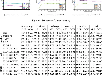
Figure 4: Influence of dimensionality
newsgroups reviews weblogs answers emails wsj
ALL OOV ALL OOV ALL OOV ALL OOV ALL OOV ALL OOV
baselines
TnT 88.66 54.73 90.40 56.75 93.33 74.17 88.55 48.32 88.14 58.09 95.76 88.30 Stanford 89.11 56.02 91.43 58.66 94.15 77.13 88.92 49.30 88.68 58.42 96.83 90.25 SVMTool 89.14 53.82 91.30 54.20 94.21 76.44 88.96 47.25 88.64 56.37 96.63 87.96 C&P 89.51 57.23 91.58 59.67 94.41 78.46 89.08 48.46 88.74 58.62 96.78 88.65 FLORS 90.86 66.42 92.95 75.29 94.71 83.64 90.30 62.15 89.44 62.61 96.59 90.37
+indi
v FLORS+HLBL 90.01 62.64 92.54 74.19 94.19 79.55 90.25 62.06 89.33 62.32 96.53 91.03FLORS+Huang 90.68 68.53 92.86 77.88 94.71 84.66 90.62 65.04 89.62 64.46 96.65 91.69 FLORS+GloVe 90.99 70.64 92.84 78.19 94.69 86.16 90.54 65.16 89.75 65.61 96.65 92.03 FLORS+CW 90.37 69.31 92.56 77.65 94.62 84.82 90.23 64.97 89.32 65.75 96.58 91.36 FLORS+W2V 90.72 72.74 92.50 77.65 94.75 86.69 90.26 64.91 89.19 63.75 96.40 91.03
+meta
FLORS+CONC 91.8772.64 92.92 78.34 95.37 86.6990.69 65.77 89.94 66.90 97.31 92.69
FLORS+SVD 90.98 70.94 92.47 77.88 94.50 86.4990.75 64.8589.88 65.99 96.42 90.36 FLORS+1TON 91.53 72.84 93.58 78.19 95.65 87.62 91.36 65.36 90.31 66.48 97.66 92.86 FLORS+1TON+ 91.5272.34 93.14 78.32 95.65 87.29 90.77 65.28 89.93 66.72 97.14 92.55 Table 5: POS tagging results on six target domains. “baselines” lists representative systems for this task, including FLORS. “+indiv / +meta”: FLORS with individual embedding set / metaembeddings. Bold means higher than “baselines” and “+indiv”.
would not make sense to replace these OOV em-beddings computed by 1TON+ with embeddings computed by “RND/AVG/ml”. Hence, we do not report “RND/AVG/ml” results for 1TON+.
Table 4 shows four interesting aspects. (i) MU -TUALLEARNINGhelps much if an embedding set has lots of OOVs in certain task; e.g., MUTUAL -LEARNING is much better than AVG and RND on RW, and outperforms RND considerably for CONC, SVD and 1TON on analogy. However, it cannot make big difference for HLBL/CW on analogy, probably because these two embedding sets have much fewer OOVs, in which case AVG and RND work well enough. (ii) AVG produces bad results for CONC, SVD and 1TON on anal-ogy, especially in the syntactic subtask. We notice that those systems have large numbers of OOVs in word analogy task. If for analogy “ais tobascis
[image:8.595.80.516.120.444.2]met-rics. Comparing 1TON-ml with 1TON+, 1TON+ is better than “ml” on RW and semantic task, while performing worse on syntactic task.
Figure 4 shows theinfluence of dimensionality
dfor SVD, 1TON and 1TON+. Peak performance for different data sets and methods is reached for d ∈ [100,500]. There are no big differences in the averages across data sets and methods for high enough d, roughly in the interval [150,500]. In summary, as long asdis chosen to be large enough (e.g.,≥150), performance is robust.
6.2 Domain Adaptation for POS Tagging
In this section, we test the quality of those individ-ual embedding embedding sets and our metaem-beddings in a Part-of-Speech (POS) tagging task. For POS tagging, we add word embeddings into FLORS7 (Schnabel and Sch¨utze, 2014) which is
the state-of-the-art POS tagger for unsupervised domain adaptation.
FLORS tagger. It treats POS tagging as a
window-based (as opposed to sequence classifica-tion), multilabel classification problem using LIB-LINEAR,8a linear SVM. A word’s representation
consists of four feature vectors: one each for its suffix, its shape and its left and right distributional neighbors. Suffix and shape features are standard features used in the literature; our use of them in FLORS is exactly as described in (Schnabel and Sch¨utze, 2014).
Letf(w)be the concatenation of the two distri-butional and suffix and shape vectors of wordw. Then FLORS represents tokenvi as follows:
f(vi−2)⊕f(vi−1)⊕f(vi)⊕f(vi+1)⊕f(vi+2) where⊕is vector concatenation. Thus, tokenviis
tagged based on a 5-word window.
FLORS is trained on sections 2-21 of Wall Street Journal (WSJ) and evaluate on the devel-opment sets of six different target domains: five SANCL (Petrov and McDonald, 2012) domains – newsgroups, weblogs, reviews, answers, emails – and sections 22-23 of WSJ for in-domain testing.
Original FLORS mainly depends on distribu-tional features. We insert word’s embedding as thefifthfeature vector. All embedding sets (except for 1TON+) are extended to the union vocabulary by MUTUALLEARNING. We test if this additional feature can help this task.
Table 5 gives results for some
representa-7cistern.cis.lmu.de/flors(Yin et al., 2015) 8liblinear.bwaldvogel.de(Fan et al., 2008)
tive systems (“baselines”), FLORS with individ-ual embedding sets (“+indiv”) and FLORS with metaembeddings (“+meta”). Following conclu-sions can be drawn. (i) Not all individual embed-ding sets are beneficial in this task; e.g., HLBL embeddings make FLORS perform worse in 11 out of 12 cases. (ii) However, in most cases, embeddings improve system performance, which is consistent with prior work on using embed-dings for this type of task (Xiao and Guo, 2013; Yang and Eisenstein, 2014; Tsuboi, 2014). (iii) Metaembeddings generally help more than the in-dividual embedding sets, except for SVD (which only performs better in 3 out of 12 cases).
7 Conclusion
This work presented four ensemble methods for learning metaembeddings from multiple embed-ding sets: CONC, SVD, 1TON and 1TON+. Experiments on word similarity and analogy and POS tagging show the high quality of the metaembeddings; e.g., they outperform GloVe and word2vec on analogy. The ensemble meth-ods have the added advantage of increasing vo-cabulary coverage. We make our metaem-beddings available athttp://cistern.cis. lmu.de/meta-emb.
Acknowledgments
We gratefully acknowledge the support of Deutsche Forschungsgemeinschaft (DFG): grant SCHU 2246/8-2.
References
Mohit Bansal, Kevin Gimpel, and Karen Livescu. 2014. Tailoring continuous word representations for
dependency parsing. InProceedings of ACL, pages
809–815.
Yoshua Bengio, R´ejean Ducharme, Pascal Vincent, and Christian Janvin. 2003. A neural probabilistic
lan-guage model.JMLR, 3:1137–1155.
Elia Bruni, Nam-Khanh Tran, and Marco Baroni.
2014. Multimodal distributional semantics. JAIR,
49(1-47).
Yanqing Chen, Bryan Perozzi, Rami Al-Rfou, and Steven Skiena. 2013. The expressive power of word
embeddings. InICML Workshop on Deep Learning
for Audio, Speech, and Language Processing. Ronan Collobert and Jason Weston. 2008. A unified
architecture for natural language processing: Deep
neural networks with multitask learning. In
John Duchi, Elad Hazan, and Yoram Singer. 2011. Adaptive subgradient methods for online learning
and stochastic optimization. JMLR, 12:2121–2159.
Rong-En Fan, Kai-Wei Chang, Cho-Jui Hsieh, Xiang-Rui Wang, and Chih-Jen Lin. 2008.
LIBLIN-EAR: A library for large linear classification. JMLR,
9:1871–1874.
Lev Finkelstein, Evgeniy Gabrilovich, Yossi Matias, Ehud Rivlin, Zach Solan, Gadi Wolfman, and Ey-tan Ruppin. 2001. Placing search in context: The
concept revisited. In Proceedings of WWW, pages
406–414.
Guy Halawi, Gideon Dror, Evgeniy Gabrilovich, and Yehuda Koren. 2012. Large-scale learning of
word relatedness with constraints. InProceedings
of KDD, pages 1406–1414.
Felix Hill, KyungHyun Cho, Sebastien Jean, Coline Devin, and Yoshua Bengio. 2014. Not all neural
embeddings are born equal. In NIPS Workshop on
Learning Semantics.
Felix Hill, Kyunghyun Cho, Sebastien Jean, Coline Devin, and Yoshua Bengio. 2015a. Embedding word similarity with neural machine translation. In Proceedings of ICLR Workshop.
Felix Hill, Roi Reichart, and Anna Korhonen. 2015b. Simlex-999: Evaluating semantic models with
(gen-uine) similarity estimation. Computational
Linguis-tics, pages 665–695.
Eric H Huang, Richard Socher, Christopher D Man-ning, and Andrew Y Ng. 2012. Improving word representations via global context and multiple word
prototypes. InProceedings of ACL, pages 873–882.
Quoc V Le and Tomas Mikolov. 2014. Distributed
representations of sentences and documents. In
Pro-ceedings of ICML, pages 1188–1196.
Yong Luo, Jian Tang, Jun Yan, Chao Xu, and Zheng Chen. 2014. Pre-trained multi-view word
embed-ding using two-side neural network. InProceedings
of AAAI, pages 1982–1988.
Minh-Thang Luong, Richard Socher, and Christo-pher D Manning. 2013. Better word representa-tions with recursive neural networks for
morphol-ogy. InProceedings of CoNLL, volume 104, pages
104–113.
Tomas Mikolov, Kai Chen, Greg Corrado, and Jeffrey Dean. 2013a. Efficient estimation of word
repre-sentations in vector space. InProceedings of ICLR
Workshop.
Tomas Mikolov, Ilya Sutskever, Kai Chen, Greg S Cor-rado, and Jeff Dean. 2013b. Distributed representa-tions of words and phrases and their
compositional-ity. InProceedings of NIPS, pages 3111–3119.
George A Miller and Walter G Charles. 1991.
Contex-tual correlates of semantic similarity. Language and
cognitive processes, 6(1):1–28.
Andriy Mnih and Geoffrey E Hinton. 2009. A scalable
hierarchical distributed language model. In
Pro-ceedings of NIPS, pages 1081–1088.
Jeffrey Pennington, Richard Socher, and Christopher D Manning. 2014. Glove: Global vectors for word
representation. Proceedings of EMNLP, 12:1532–
1543.
Slav Petrov and Ryan McDonald. 2012. Overview of
the 2012 shared task on parsing the web. In
Pro-ceedings of SANCL, volume 59.
Pushpendre Rastogi, Benjamin Van Durme, and Raman Arora. 2015. Multiview LSA: Representation
learn-ing via generalized CCA. InProceedings of NAACL,
pages 556–566.
Tobias Schnabel and Hinrich Sch¨utze. 2014. FLORS: Fast and simple domain adaptation for
part-of-speech tagging. TACL, 2:15–26.
Ilya Sutskever, Oriol Vinyals, and Quoc VV Le. 2014. Sequence to sequence learning with neural
net-works. InProceedings of NIPS, pages 3104–3112.
Yuta Tsuboi. 2014. Neural networks leverage
corpus-wide information for part-of-speech tagging. In
Pro-ceedings of EMNLP, pages 938–950.
Joseph Turian, Lev Ratinov, and Yoshua Bengio. 2010. Word representations: a simple and general method
for semi-supervised learning. In Proceedings of
ACL, pages 384–394.
John Wieting, Mohit Bansal, Kevin Gimpel, and Karen
Livescu. 2015. From paraphrase database to
compositional paraphrase model and back. TACL,
3:345–358.
Min Xiao and Yuhong Guo. 2013. Domain adaptation for sequence labeling tasks with a probabilistic
lan-guage adaptation model. InProceedings of ICML,
pages 293–301.
Yi Yang and Jacob Eisenstein. 2014. Unsupervised
domain adaptation with feature embeddings. In
Pro-ceedings of ICLR Workshop.
Wenpeng Yin and Hinrich Sch¨utze. 2015. Multichan-nel variable-size convolution for sentence
classifica-tion. InProceedings of CoNLL, pages 204–214.
Wenpeng Yin, Tobias Schnabel, and Hinrich Sch¨utze. 2015. Online updating of word representations for
part-of-speech taggging. InProceedings of EMNLP,
pages 1329–1334.