Analysis of flow processes at the downstream side of various river measures using 1D and 2D flow models

(1)

Anal

ys

i

s

of

ow

pr

oces

s

es

at

t

he

down-s

t

r

eam

s

i

de

of

var

i

ous

r

i

ver

meas

ur

es

us

i

ng

1D-

and

2D ow

model

s

Mas

t

er

Thes

i

s

Mi

chi

el

Cl

ement

s

(2)

(3)

Analysis of flow process at the

downstream side of various

river measures using 1D- and

2D flow models

Master Thesis Michiel Clements

August 2016

Graduation Committee:

Ir. R.P. van Denderen

University of Twente

Dr. Ir. J.S. Ribberink

University of Twente

Dr. A.P. Tuijnder

Arcadis

(4)

(5)

Preface

In this report the result of the research project that I did during 6 months at Arcadis can be found. During this time I have learned many different subjects regarding river flow modeling, river flow processes and clarifying these complicated subjects in a report. Furthermore, I have learned about what it is like to work in the civil engineering field and more specifically to work at Arcadis. I have enjoyed my time very much and I therefore want to thank the company for giving me this opportunity.

I also want to thank Arjan Tuijnder as my daily supervisor at Arcadis. Thank you for being there almost every day to answer my questions. I have learned a lot from you. You always required to formulate complicated questions as clear as possible. This has helped me a lot in writing the report. Thank you Pepijn for your help during this period too. You were always willing to help and check formulas if I asked to. We were both situated in a different location so our communication was mainly by email. And yet your response was always very quick which is very much appreciated. Thank you Bart for your help. You always were able to clearly explain questions regarding complicated subjects such as turbulence or non-hydrostatic flow. I want to thank dhr. Ribberink. Your feedback was very constructive and has helped to reshape my report in a structured way. Your flexibility regarding the research process is very much appreciated. I finally want to thank my lovely wife Jacomijn for her support. Especially in the last stage of my research almost my whole life was devoted to it. And still you always helped and supported me and never complained about me doing my work. I’m very grateful and astonished by the way you have helped me through.

I want to thank you all very much. Above all I want to thank God for His help. He has helped and supported me day after day. I have always wanted to do a research about rivers because these creations have always been very intriguing to me. Therefore, my greatest desire is to adore the most amazing river there ever will be, which is the river in heaven:

Revelation 22:10. Then the angel showed me the river of the water of life, as clear as crystal, flowing from the throne of God and of the Lamb

(6)

Summary

After implementation of river measures in sub-critical flow, the water level upstream of the measure decreases. However, at the downstream boundary of these measures the water level tends to increase. This is observed as a local peak. In this research the existence of this peak is investigated.

This is undertaken by introducing two schematized river measures: a widening measure and a deepening measure. The focus was mainly on the downstream side of these measures.

It is shown that the flow processes that cause the peak at the downstream boundary of the both measures can be explained by the Bernoulli equation. Bernoulli states that when the flow decelerates, the water level increases. In sub-critical flow, the effects of the river measures are only experienced upstream. Implementing the deepening measure, no changes thus occur far downstream of this measure. When going from that point in upstream direction, the flow decelerates since the river profile expands. Bernoulli explains that due to this deceleration the water level increases in upstream direction.

A similar process occurs at the downstream side of the schematized widening measure. However, at the downstream boundary of the measure, the lateral change of the river profile causes lateral flow velocities towards the axis of the river. This has a significant influence on the shape of the peak. Furthermore, turbulence tends to be an important flow process and has an increasing effect on the peak.

There is also an analysis undertaken on the used grid size in flow models. Regarding the deepening measure, using a smaller grid size then length of the step in the bed, no significant changes occur. However, using a larger grid than this length results in a smaller peak and should therefore not be used. Regarding the lateral flow constriction, when a grid size is used that is smaller than 1 * db/dx, no significant change occurs. When using a larger grid size the peak is overestimated.

(7)

1 Introduction

1.1 Background

The Netherlands is located in the middle of a delta, therefore the Dutch have had to deal with water for many centuries. They have to fight and work with water coming from upstream countries in the east as well as water from the sea in the west. Furthermore, as is shown in Figure 1, the country is subsiding while the level of the sea is rising causing many parts of the Netherlands to be below sea level. This has caused many floods such as in the ‘Zuiderzeegebied’ (1916) and in Zeeland (1953), for example. The latter led to the establishment of the ‘Delta-committee’ in 1958 which was assigned to come up with measures necessary to preventing further floods, especially of the same magnitude.

Figure 1; Schematic representation of subsidence and sea level rise throughout the years (Verhallen, 2001)

Since the establishment of this committee, many measures have been applied to protect the country. There have been many developments near the coast to prevent the inundation of sea water, and inland likewise for river water. Some examples of these measures are shown in Figure 2.

Figure 2; examples of measures in rivers

(10)

flow processes included in calculations. This, in turn, has led to more predictions and a better understanding of flow behavior in river systems. However, despite the advantages of using advanced models, the overview of all processes in the model can be obscured. This might mean some effects in the model output are much less easily understood.

1.2 The downstream peak

Most flow models used to analyze the effect of river measures are based on the Shallow Water Equations, or Saint Vanant equations. After the implementation of various river measures in these flow models, a peak occurs at the downstream side of the river measure in the results of these models. This occurs after examining the implementation of various measures such as constructing a side-channel (Herik & Rooy, 2007), widening measures (Diermanse, 2004b) and deepening measures (Linde, 2008).

All these measures have one common characteristic: the peak exists at the location where the flow is constricted, either horizontally or vertically. An example of this peak is shown in Figure 3.

Figure 3; water level difference after implementing side channel

In this Figure the difference of the water level is shown between the situation with and without the implementation of the side channel. In this case, the side channel flows into the river at rkm 980. It is clearly visible that a peak occurs at rkm 980 which is exactly at the constricted location. The peak is thus defined as the increased part of the water level after implementation of a river measure compared to the situation without this measure. In this report, the situation without the measure is called the reference situation.

1.3 Policy regarding the downstream peak

The downstream peak is limited by the ‘Rivierkundig beoordelingskader’ (RBK) or ‘hydraulics assessment framework’ (Kroekenstoel, 2014). This policy document is decisive when river interventions are implemented in the Netherlands. According to this document, the increase of water level after implementing measures is only allowed if:

(11)

 The design is ‘optimized’, which means that the most optimal design is chosen in order to reduce the peak as much as possible without significantly changing the decreasing effect of the water level of the intervention.

 The surface of the increased triangle is much smaller than the decreased triangle (see Figure 4). In practice this means that the decreasing effect must be 50 to 100 times larger than the increasing effect.

 The peak does not reach outside the boundaries of the intervention.

Figure 4; increased triangle and decreased triangle

1.4 Research motivation and questions

As stated above, the peak occurs in the result of flow models. However, until now it has been uncertain whether this peak is accurately represented. The flow models are based on several simplifications. For example, there are certain assumptions about the way turbulence due to friction or changes in the river profile are modeled. It is also assumed that the pressure distribution is hydrostatic in all circumstances. Furthermore, the analytical equations which are the basis of these flow models are discretized using a specific step size. In practice, the minimum step size is 20 m, which might leave out detailed information about the dimensions of the river measure. Until now it is uncertain to what extent this influences the way the peak is represented. Therefore, a more detailed research on these processes and their relation to the peak is necessary.

1.4.1 Problem definition

Considering the different aspects above, the problem definition is as follows: It is uncertain whether a peak occurring in the result of flow models at the downstream side of river measures is accurately represented since, on the one hand, these flow models are based on several simplifications and, on the other hand, spatial detailed information of the river measures is left out.

1.4.2 Objective and Research questions

The objective of this study is to gain insight into the relation between flow processes around the downstream side of river measures and the downstream peak, and also how this can be used to reduce the dimensions of the peak in the preliminary design phase of constructing a side channel.

For this research, two research questions are examined. The first question focuses on the cause of the peak and the second question focuses on different ways to reduce the dimensions of the peak.

1. Is the downstream peak accurately represented in the flow models that are applied to design river measures?

a. What flow process(es) are of importance at the downstream side of various river measures?

b. What is the effect of the step size in the discretized equations on the representation of these flow processes?

(12)

1.5 Research approach

1.5.1 Schematized river measures

According to several reports, the downstream peak appears at the downstream boundary of different river measures i.e. at the location where the flow is constricted (see introduction, subsection 1.2). In order to examine the flow at the location of the constriction, two basic types of measures are introduced: a widening measure and a deepening. In both measures, the flow is constricted at the downstream boundary.

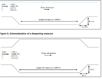
The analysis of this research is done for a river section with typical dimensions of a river in the Netherlands. These dimensions are inspired by the Waal river, which discharges 2/3 of the discharge entering the river Rhine near Lobith. Since the design-discharge is 16000 m3/s at Lobith, the discharge of the Waal in that scenario is 10667 m3/s. Furthermore, the average width of the Waal-river is approximately 360 m. The typical bed slope of rivers in the Netherlands is 1m / 10 km. Furthermore, a Chézy roughness value of 50 m1/2/s is chosen as a typical roughness value for the river Waal.

[image:12.612.73.431.297.575.2]

The deepening measure concerns the deepening of the river bed of 1 m over a section of 1000 m (see Figure 5), while the widening measure concerns an expansion of the summer bed of 20 meters at both sides of the river over a section of 1000 m (see Figure 6).

Figure 5; Schematization of a deepening measure

Figure 6; Schematization of a widening measure

1.5.2 Analysis of flow processes around the downstream side of various river measures

For this research, three different model configurations are introduced. Each model configuration represents a set of different terms of the Reynolds Averaged Navier Stokes equations. By subsequently applying each model configuration to the schematized river measures, it is analyzed what terms and therefore what flow processes are of importance at the downstream side of these measures. The model configurations that are examined are as follows:

(13)

Model configuration I: 1D - Bernoulli

In this research, effects on the flow around sudden changes of the river profile are examined. These sudden changes cause the water flow to accelerate locally. This might cause the acceleration term to be more important than the bottom friction term. If this is the case, the flow is described by the Bernoulli equation without head loss. This is applied to both schematized river measures.

Model configuration II: 1D – Bélanger

In model configuration II the influence of the friction term is examined. This is done by adding the friction term to the previous configuration. The flow is then described with the Bélanger equation or ‘Back-water curve method’. After applying this to both schematized river measures, the model results are compared to the results of the previous configuration. This way it is examined whether the Bernoulli equation is still the right way of describing the flow at the schematized river measure (and more importantly around the downstream side), or that the friction term plays an important role and may thus not be neglected.

Model configuration III: 2D modeling

In configuration III the effect of adding a second dimension to the flow model is studied. Instead of using a 1D model a 2D model is applied.

For the deepening measure two effects are studied: 1) the influence of turbulence and 2) the influence of the hydrostatic pressure assumption

First the effect of turbulence is examined. This is done by introducing the vertical k – epsilon turbulence model. By comparing the results with k- epsilon model to the results of the previous configuration, conclusions will be drawn on the influence of turbulence. Secondly, it is examined whether the hydrostatic assumption is valid. When vertical velocities are large, the pressure distribution is non-hydrostatic. It is uncertain what the magnitudes of the vertical flow velocities at the step in the bed are. Therefore it is also uncertain whether the hydrostatic pressure assumption is still right. It is thus examined what the behavior of the flow is when non – hydrostatic effects are also included. Both the effect of vertical mixing and the non – hydrostatic effect will be analyzed in a 2DV model by introducing space steps in x – direction and several layers in z – direction.

Regarding the widening measure, two effects are studied 1) the influence of lateral flow velocities and 2) the influence of the horizontal mixing term.

First the effect of the lateral flow component is examined. This is done by including both the longitudinal as well as the lateral flow velocities in a 2DH flow model with a grid with cells of 2 m x 2 m. As will be shown in the report, with this grid size the results of the flow are converged, i.e. using a smaller grid size does not have a significant influence on the results anymore. By comparing these results to the results generated with the 1D model, conclusions will be drawn on the influence of the lateral flow velocities.

Secondly, the influence of the horizontal mixing term is examined. This is done in two ways. First a spatially variable horizontal eddy viscosity is used, namely the Horizontal Large Eddy Simulation model (HLES). This is the most advanced way of estimating the horizontal eddy viscosity in this research. Comparing the results of the model run with HLES included to the model run without turbulence model thus gives insight into the effect of turbulence. However, in practice, performing a HLES simulation is very computationally intensive. Therefore often a spatially constant horizontal eddy viscosity is used. This is also done in this research and this is the second way of examining the mixing term. The magnitude of the constant horizontal eddy viscosity is based on an estimation presented by Madsen et al (1988). By comparing these results to the results obtained with HLES, it is investigated how well the turbulence is represented by the second turbulence model.

(14)

Deepening measure

Model

Dimensions

taken Turbulence Investigated Configuration into account model

(vertical)

subject

I 1D - Bernoulli II 1D - Belanger

III Quasi - 2DV k - epsilon Influence of turbulence Full - 2DV k - epsilon Non - hydrostatic effects

Table 1; over view of model configurations applied to the deepening measure

Widening measure

Model

Dimensions

taken Turbulence Investigated Configuration into account model (horizontal) subject

I 1D - Bernoulli II 1D - Belanger

III

2DH Constant, = 0 m/s2 _{Influence of lateral flow} 2DH HLES Influence of turbulence

2DH

Constant = 0.6 m/s2, estimated with Madsen et al (1988)

Reliability of using a spatially constant

hori-zontal eddy viscosity

Table 2; overview of model configurations applied to the widening measure

1.5.3 Analysis of grid size in flow models

For the analysis of the flow processes, a grid size of 2 m x 2 m is used. In this research it is investigated whether the size of the grid has an influence on the representation of the flow processes that are of importance at the downstream side of the river measure. This is done as follows: 1) by decreasing the grid size and 2) by increasing the grid size used.

First the grid size is decreased. This is done until the results generated with the flow model converges. This converged solution is compared to the solution generated with using a grid size of 2 m x 2 m. This way conclusions are drawn on the influence of the grid size on the representation of the flow processes.

Second, the grid size is increased to 10 m x 10 m and to 40 m x 40 m. The latter grid size is sometimes used in practice when river flow in the Netherlands is modeled. This is thus the worst – case scenario in which the fewest details are taken into account. By comparing these results to the results with the analysis of 2 m x 2 m, conclusions are drawn on the effect of using a large grid size.

1.5.4 Reducing the dimensions of the peak

With the results of the previous subsections it is investigated what the cause of the peak is. Subsequently is it examined how the dimensions of the peak can be reduced in the preliminary design phase of a side channel. This is done by focusing on the flow processes that cause a peak in a real world case.

(15)

[image:15.612.73.390.68.385.2]

Figure 7; Project ‘Scheller and Oldeneler Buitenwaarden’ near Zwolle

It is shown that the side-channel is constructed in the floodplain of the IJssel. The flow direction is from South East to North West. At the downstream side of the side channel, the channel is connected to the main stream of the IJssel, and at the upstream side the channel is closed off with a small dike. Only with high water events the water flows over this dike into the side channel. This is to prevent the side channel from sedimentation, which occurs at low flow velocities (The Open University, 1999).

The summer bed of the IJssel river is approximately 160 m wide, and the winterbed 100 m wide. The winterbed at the location where the side channel is constructed is much wider, i.e. it is 600 m at the east side. The length of the wide winterbed is approximately 3.5 km. The floodplains are 5 meters above the summer bed.

The length of the side channel is approximatlely 2 km and the width is 100 m. The bed level of the side channel is 3 m below the bed level of the summer bed.

The design discharge is 16000 m3/s at lobith which corresponds to a dicharge of 1800 m3/s of the IJssel. The bed slope is approximately 1 m / 10 km.

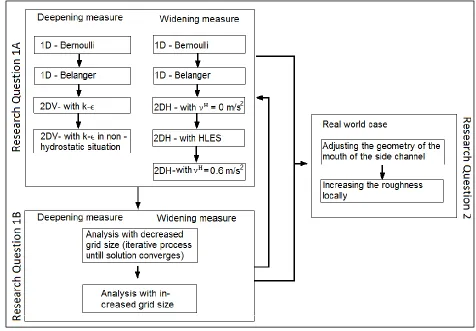
1.5.5 Summary of research approach

(16)

[image:16.612.66.542.114.445.2]

Figure 8; Summary of research approach

This is input for research question 2. Here some measures are proposed to reduce the dimensions of the peak.

1.6 Outline report

This report is outlined in Table 3. The first chapter considers the background to the mathematical equations describing water flow. It demonstrates how specific assumptions result in the Bernoulli and Bélanger equation as well as the equations describing both 2DH and 2DV flow. It considers what the processes are behind both the k – epsilon and the HLES model.

The second chapter conveys the methodology used (either numerically and/or analytically) for both schematized river measures. It is shown how the solutions are implemented in the software used (Matlab, WAQUA and SWASH).

(17)

Chapter 5 builds on the results presented in Chapter 4, reducing the dimensions of the peak. This is applied to the real-world case. Here the second research question is examined.

Chapter 6 draws the conclusions from the results and the discussion and provides recommendations.

Chapter

Research question examined

2. Flow theory and governing equations

1 3. Solution method and model set up

4. Results

5. Practical Application 2

6. Conclusions, Discussion

and Recommendations

(18)

2 Flow Theory

This chapter examines flow in general and more specifically how water flow is modeled. In order to do that, first the Navier-Stokes equations are introduced. However, performing direct computations using these equations is very computationally intensive. The existence of a general solution of these equations is even one of the Millennium Problems. (Fefferman, 2002). Therefore, it is shown how Reynolds applied an averaging procedure to the equations making calculations feasible. This procedure is shown resulting in momentum equations for flow in general. After that, it is shown how the resulting equations are applied to water flow specifically, by introducing key assumptions regarding water flow.

2.1 Navier-Stokes equations

Throughout many centuries researchers have tried to understand and predict the behavior of fluid flow. One of the most and comprehensive mathematical descriptions used in order to obtain this is introduced by Navier (1785-1836) and Stokes (1819-1903) by introducing a balance of momentum of a fluid, the so called incompressible Navier-Stokes equations:

⏟ * + ⏟ ⏟ ⏟ ( ) ⏟ (2.1) ⏟ * + ⏟ ⏟ ⏟ ( ) ⏟ (2.2) ⏟ * + ⏟ ⏟ ⏟ ( ) ⏟ (2.3) Where

Term 1: the temporal acceleration Term 2: the spatial acceleration Term 3: the pressure force Term 4: the viscous forces Term 5: the gravity force

With

g gravitational acceleration [m/s2] u velocity in x-direction [m/s]

t time [s]

v velocity in y-direction [m/s] w velocity in z-direction [m/s]

moleculair viscosity [kg/(m s)] density of water [kg/m3] p pressure [kg/(m s2)]

2.2 Reynolds averaged Navier-Stokes equations

(19)

Figure 9; Reynolds averaging principle

Therefore, Reynolds proposed to average the NS equations over time by introducing the instantaneous velocities, u’, v’ and w’ as:

u = U + u’ (3.4)

v = V + v’ (3.5)

w = W + w’

(3.6)

In which:

U = time – averaged velocity defined as ∫ in x-direction u’= instantaneous velocity fluctuation in x - direction

Similar variables are defined for the variables in x and y direction. Substituting this in the NS-equations and averaging yields the Reynolds Averaged Navier Stokes equations and is defined as follows (White, 2009). * + ( ₎ ( ) (

) _(2.7)

* + ( ) ( ₎ (

) _(2.8)

* + ( ) ( ) ( ₎ (2.9)

These equations form the basis of computational flow dynamics in various academic fields such as natural sciences (Sinha et al, 1998) and aerospace engineering (Potturi & Edwards, 2012). In this research the focus is on water flow in rivers, which means that certain assumptions are done to simplify the equations. However, before focusing on shallow water flow, first it is shown how the shear stresses are modeled.

In equation 2.7, , and are called the turbulent stresses, and the gradients in al velocity directions are the laminar stresses. For the x-direction this yields (White, 2009):

(2.10)

(20)

, and (2.11)

With [m2/s] the horizontal eddy viscosity and [m2/s] the vertical eddy viscosity. The horizontal and vertical eddy viscosities are much larger than the dynamic viscosity , therefore is negligible. Furthermore, the spatial resolution of the grid and time steps are much larger than the typical length and time scales of turbulent motions, so the eddy viscosities [m/s2] and [m/s2] are both assumed to be constant (Uittenbogaard, 1992).

A similar procedure as for the momentum in x-direction can be done for the momentum equations in y and z direction. Furthermore gx=gy=0, since the axis are chosen such that the z-axis is in the same direction as

gz. With this, the 3D momentum equations for incompressible water flow in x, y and z direction are defined

as follows: *

+ _(2.12)

*

+ _(2.13)

*

+ (2.14)

Applying the Boussinesq assumption, the complexity of the RANS equations is thus reduced significantly.

2.3 Shallow water flow: the assumption of shallowness and steadiness

The RANS equations can be further reduced to the specific case of shallow water flow, such as in river systems. In shallow water, the fluid motions are predominantly horizontal. Therefore, the vertical acceleration is very small and is therefore negligible. Under that assumption, the vertical momentum equation is reduced to the following equation:

This is also known as the hydrostatic pressure distribution. By integrating this equation over z and assuming p0 = 0 (atmospheric pressure), the pressure distribution is as follows:

( ) (2.15)

In here z is the distance from the water level zw to a reference point (see figure 10).

Figure 10; Definition of water level compared to reference point

(21)

( ) ( ) (2.16)

Substituting the hydrostatic pressure distribution into the RANS equations and averaging over the depth gives the Shallow Water Equations or Saint Vanant Equations. For more detailed information, see Appendix C where it is shown how the SWE are derived.

* ̅ ̅ ̅ ̅ + | ⃗⃗ | ̅ (2.17) * ̅ ̅ ̅ ̅ + | ⃗⃗ | ̅ (2.18)

Furthermore, besides the hydrostatic pressure distribution, it is also assumed that the change of momentum over time is zero, i.e.

. This means that the flow in all model configurations is assumed

to be steady.

2.4 Model configuration I: 1D - Bernoulli

The most simplified model configuration considered in this research is the Bernoulli equation without head loss. The assumptions on the RANS equations are as follows:

Assumption 1: _{All derivatives in lateral and vertical direction are zero, i.e.}

Assumption 2: The lateral velocity v [m/s] and vertical velocity w [m/s] are much smaller than the velocity in direction of the flow u [m/s], and therefore v=w=0

Assumption 3: Both the horizontal and the vertical turbulence is neglected

The flow is also assumed to be frictionless, since no eddy viscosities are considered. The reduced momentum equations are then as follows:

(2.19) (2.20)

Substituting equation 2.20 in equation 2.19 and integrating over x gives the Bernoulli equation (see appendix A for the derivation of Bernoulli). This is a depth averaged flow and thus a 1D configuration:

̅

(2.21)

Where

̅ [m/s] velocity in x-direction [m2/s] gravitational acceleration

h [m] water depth

zb [m] bed level

(22)

2.5 Model Configuration II: 1D - Bélanger

The subsequent model configuration considered in this research is described by Belanger, in which the friction term is included in the mathematical description. The assumptions on the RANS equations are as follows:

Assumption 1: _{All derivatives in lateral direction are zero, i.e.}

Assumption 3: The horizontal turbulence is neglected

The RANS equations are then reduced to the following momentum equations:

( ) _(2.22)

(2.23)

In this configuration, the flow is averaged over the depth and thus is this a 1D model. In depth averaged mode, the vertical eddy viscosity is related to the friction as is shown in appendix C. Substituting this in equation 2.22 yields:

̅ ̅ ̅ (2.24) Where

C [m1/2/s] Chézy coefficient h0 [m] Water depth

ib Bottom slope

Furthermore, the following continuity relation is defined:

̅

(2.25)

Substituting equation 2.25 in equation 2.24 and assuming that the change of width over x is zero, i.e.

gives the Bélanger equation. The derivation of this equation is shown in appendix D.

* + (2.26) With [

√ ] = equilibrium depth (2.27)

* + = critical depth (2.28)

Where

(23)

h0 [m] Water depth

ib Bottom slope

2.6 Model configuration III – 2D modeling

In all previous configurations, the flow is considered in 1 dimension. In this model configuration the 2D effects are examined. At the deepening measure the effects in vertical direction are examined and at the widening measure the effects in lateral direction are examined.

The 2D effects that are investigated around the downstream side of the deepening measure concerns the influence of the vertical mixing term and the effect of vertical flow. First the assumptions on the RANS equations are shown for the situation in which the influence of turbulence is considered:

Assumption 1: _{All derivatives in lateral direction are zero, i.e.}

Assumption 3: The horizontal turbulence is neglected since there are no lateral changes of the river profile and wall friction is neglected

The momentum equation in y-direction is then assumed to be 0, while the momentum equation in z- and x-direction are respectively as follows.

(hydrostatic situation) (2.29)

( ) _(2.30)

Again, the hydrostatic pressure distribution is substituted in the equation representing momentum in x – direction:

( ) (2.31)

Differently from the previous model configuration, the vertical mixing term is only related to Chézy at the boundary condition located at the bottom, since multiple layers are defined (thus non-depth averaged). Instead, the flow is averaged laterally. It is thus solved in quasi - 2DV mode, in which longitudinal differences in vertical direction are taken into account, but in which the vertical flows are neglected.

For the situation in which the effect of the vertical flow is considered, the assumptions are as follows:

Assumption 1: There is no horizontal turbulence since there is no wall friction and lateral changes in the river profile

Assumption 2: All lateral velocities can be neglected since no lateral changes occur in the river profile, so v = 0 and

= 0

Therefore, the governing equations are as follows:

*

(24)

*

+ (2.33)

These set of equations represent thus momentum in x and momentum in z direction. The flow is averaged laterally in which vertical and longitudinal flow velocities are taken into account. This is thus a full-2DV analysis (instead of quasi – 2DV represented by equation 2.31). Differently from the previous configurations, the hydrostatic flow regime is not valid anymore. With this set of equation, non – hydrostatic effect are investigated where the flow is constricted at the downstream boundary of the deepening measure.

Regarding the downstream boundary of the widening measure, the assumptions on the RANS equations are as follows:

Assumption 1: The velocity w [m/s] is much smaller than the velocity in direction of the flow u [m/s] and v [m/s], and therefore w = 0.

Applying these assumptions, the following mathematical description is obtained. The momentum equations are as follows:

* + (2.34) *

+ (2.35)

(2.36)

In this configuration the velocity is averaged over the depth, and therefore the vertical diffusion term is related to the friction. With this depth – averaging procedure, the so called Shallow Water Equations or Saint Venant Equations are obtained (see Appendix C) (Randall, 2006):

* ̅ ̅ ̅ ̅ + | ⃗⃗ | ̅ (2.37) * ̅ ̅ ̅ ̅ + | ⃗⃗ | ̅ (2.38)

These equations represent a 2DH set of equations in which the lateral and longitudinal flow velocities both differ in longitudinal as lateral direction, but not in vertical direction.

Introduction to turbulence modeling

The effect of turbulence is modeled by the diffusivity terms. Diffusion is the movement of matter at high concentration to a region of lower concentration. This also applies to momentum: When there is a region with high concentration of momentum and a region of low concentration, the effect of diffusivity is that it reduces the gradient. This behavior is also observed when turbulence is present in the flow. The flow is then more mixed and differences in momentum are reduced. Therefore, including the diffusivity terms is a way of including the behavior of turbulence.

(25)

The k – epsilon turbulence model

The model used for determining vertical eddy viscosities is the so called turbulence model (Rodi, 1984). This model consists of two transport equations. The first transported variable determines the energy that is available in the turbulence and is called the specific turbulent kinetic energy [m2/s2]. The other transported variable is the dissipation [m2/s3] which determines the rate of dissipation of the turbulent kinetic energy [m2/s2].

The energy balance of the turbulent kinetic energy is as follows (Rodi, 1984):

⏟ ( ) ⏟ [ ] ⏟ ⏟ – ⏟ (2.39)

And for the dissipation energy (Rodi, 1984):

⏟ ( ) ⏟ [ ] ⏟ ⏟ ( ) ⏟ (2.40) With:

[m2/s] (2.41)

Equation 2.39 and 2.41 each consists of five terms. The terms represent the following processes.

Term 1: rate of change of or over time Term 2: transport of or by convection Term 3: transport of or by diffusion Term 4: rate of production of or Term 5: rate of destruction of or

The production term consists of a Buoyance term Bk which represents the exchange between turbulent

kinetic energy and potential energy and is defined by:

(2.42)

This term is only of importance in case of density differences in e.g. estuaries. Since there are no density differences incorporated in this research this Buoyance term is set to 0.

Furthermore, the production term consists of a term Pk, which represents the production of turbulent

kinetic energy and is defined by:

[(

) ( ) ]

(26)

Besides the production term, many coefficients are also included. These coefficients are determined empirically, and are shown below (Rodi, 1984):

{

For the use of the k – epsilon model, the Nikuradse Roughness height ks is introduced as the

representation of bottom friction. By introducing this, the influence of the friction is dependent on the water depth, which therefore gives a more accurate way of the influence of the bottom friction on the water flow. The relation between the Chézy value and the Nikuradse height is shown in the White-Colebrook relation:

√ ( ) (2.44)

Where

g gravitational acceleration [m/s2] C Chézy coefficient [m1/2/s] R Hydraulic radius [m]

k Nikuradse Roughness height [m]

The HLES turbulence model en the estimation of Madsen et al (1988)

The model used for generating the horizontal eddy viscosities is the Horizontal Large Eddy simulation model. This model is based on two major components: the physical turbulence that is present and the sub-grid eddy viscosity. The way turbulence is modeled is based on the Prandtl-Kolmogrov model:

√ [m

2

/s] (2.45)

Where [m2/s2] is the kinetic energy of the turbulent motion, L [m] the length scale of the geometry and is an emperical constant. The eddy viscosity is further simplified as the Elder viscosity, where ,

√ [m /s] and L = H [m] (Uittenbogaard, 1992):

( ) [m

2

/s] (2.46)

Where

= von Karman constant (=0.41) [-] ( ) friction velocity at the bottom ( = √

u [m/s])

H is the water depth [m]

Another phenomenon that is taken into account is numerical viscosity. This becomes important when a grid size is used with an order of magnitude larger than the eddies that would occur in reality. In not taking this into account, the energy dissipated in the model is less than in reality. To solve this problem, a sub-grid eddy viscosity [m/s

2

] is introduced, which takes both the magnitude of [m] as [m] into account. For more detailed information on the calculation and the mathematical background, reference is made to (Uittenbogaard, 1992).

(27)

[m

2

/s] (2.47)

The advantage of the HLES model is that it includes by default a horizontal eddy viscosity coefficient based on the local presence of turbulence and the locally used grid size. This is especially interesting in cases where a varying grid size is used. The disadvantage of this model is that it is more computationally intensive. Alternatively, a constant eddy viscosity coefficient can be used. An estimation of a constant horizontal eddy viscosity is introduced by Madsen et al (1988) as follows:

[m2/s] (2.48)

(28)

3 Model set up and software used

This chapter demonstrates how the mathematical equations represented in the previous chapter are applied to both schematized river measures. Furthermore it is shown how the equations can be solved either numerically or analytically and how they are implemented in the software used.

3.1 Model configuration I: 1D - Bernoulli

For the application of the Bernoulli equation on the deepening measure, first a relation between the velocity and the bottom level is introduced:

̅

_(3.1)

Where

q [m3/s] specific discharge h [m] water depth (= zw - zb)

Substituting this in equation 2.19 yields:

( ) (3.2)

Furthermore, the Froude-number is included. The change of water level over a distance x in relation to the Froude-number is as follows (see appendix B for the derivation):

( ) (3.3)

This equation is discretized as follows:

( )

(3.4)

Where

[m] water level along the river [m] water level at x =0 Fr0 [-] Froude number at x = 0

[m] vertical distance of step in river bed

Equation 3.4 is implemented in Matlab to describe the longitudinal variation of the water level as function of the vertical change of the river bed.

For the application of the Bernoulli equation to the widening measure, a relation between the discharge and the river width is included. For this situation, instead of a constant with b [m], a constant bed level zb

[m] is applied. The velocity is then defined as follows.

̅

_(3.5)

Q [m3/s] discharge

b [m] width of river profile

h [m] water depth

(29)

(

)

(3.6)

Since the Bernoulli equation is constant along a streamline, the solution is obtained by setting the constant at the boundary conditions equal to the constant elsewhere in the domain. Equation 3.6 is then solved numerically as follows:

( ) ( ) ( ) _(3.7)

In here, Q [m3/s] and g [m/s2] are constants and so are [m] and [m]. With this equation the longitudinal variation of the water level is described as function of the change of the river width. The software used is Matlab.

Furthermore, the change of the water level is related to the Froude number as follows (see appendix B for the derivation):

( )

(3.8)

3.2 Model Configuration II: 1D - Bélanger

3.2.1 Deepening measure

The mathematical description proposed by Bélanger can be solved analytically and numerically. In this research both methods are demonstrated. The equation is solved analytically by means of the ‘approximation according to Bresse’ (Putnam, 1948). However, the analytical approximation contains the equilibrium depth he (see equation 2.25). This equilibrium depth is proportional to √ . At the upstream

boundary of the deepening measure ib becomes negative. This means that he becomes imaginary and

therefore the analytical solution is not used for the deepening measure. Instead of defining ib, the change

of the bed level is considered to be in an infinitely small point, leaving out the effect of the changing bed. This method is also applied in practice.

When solving the equation numerically, this problem does not occur. In the numerical solution, dh/dx is proportional to (which is shown later on in this report, see e.g. equation 3.14) and therefore the solution can still be used when ib becomes negative. The equation is solved numerically by means of the

predictor corrector method (Van Rijn, 1990).

The analytical approximation thus neglects the change of the bed slope and is used to show how the problem is solved if this solution would be used. The numerical approximation is used to show whether the change of the bed slope may indeed be neglected and what flow processes are of importance at the downstream side of the measure.

Analytical solution of Bélanger using the approximation according to Bresse

The Bélanger is solved analytically with use of the approximation of Bresse, which is used when Fr2 << 1. Using the flow parameters of the both schematized river measures, the flow velocity is estimated to be around 2 m/s, and the depth to be around 15 m. The Froude-number is than:

√

(3.9)

Therefore Fr2 << 1 and the approximation method can be used. The water depth at distance from x0 is

determined as follows:

(30)

( ) ( )

(

)

(3.10)

Where

( ) [m] half adaption length (3.11)

The ‘half adaption length’ indicates at which location the water depth is exactly in between the water depth at the downstream location and the equilibrium depth.

Implementation method in Matlab

For the implementation of the analytical solution in Matlab, the computation is divided into three different sections: the section downstream of the measure, at the measure and upstream of the measure (see Figure 11). At each section the equilibrium depth changes, and so does the adaption length. For the analysis, first the situation downstream of the measure is considered, with x0 at the far left end of the

domain. When the h(x) is computed for the downstream section, the analysis is done for the section at the measure. x0 is changed to the downstream boundary of the measure, i.e. to x = 1000 m, and a new

equilibrium depth (and therefore adaption length) is computed. With this, h(x) for the section at the measure is determined. The same procedure is used for the calculation of h(x) at the upstream section of the measure.

Figure 11; model set up in Matlab for analytical solution of Bélanger

Numerical approximation of Bélanger using the predictor-corrector method

The Bélanger equation is approached numerically as follows. First, the water depth h as a function of x is discretized using a forward Taylor expansion in space, giving a second order accuracy in :

( ) ( )

| ( )

(31)

Using a numerical notation and leaving out the higher order terms this yields: | (3.13) Furthermore,

is the Bélanger equation (which is derived in appendix D) and is defined as follows:

* ( ) + ( ) (3.14)

For the discretization of the bed slope, both the forward and backward Taylor expansion in space are defined respectively as follows:

( ) ( )

| ( )

_| ₍ ₎ (3.15)

( ) ( )

| ( )

_| ₍ ₎ (3.16)

Subtracting the forward Taylor expansion from the backward Taylor expansion yields the central difference scheme of the bed level, with a third order accuracy in space.

( ) ( )

| ( )

(3.17)

Using a numerical notation and leaving out the higher order terms, the bed slope is discretized as:

|

(3.18)

Substituting equation 3.18 and equation 3.17 in equation 3.13 gives a discretized function for h as function of x. [ ( ) ] ( ) (3.19)

This numerical approach has a second order accuracy. That means that the following term is neglected:

| ( ) (3.20)

Using this term, an accuracy check is performed on the proposed numerical approach shown in equation 3.19. For this, the higher order terms are left out, since that error is always smaller than the second order term. The second order term is therefore a good representation of the error made in this model. The value for this error is estimated as follows:

( | | ) (3.21)

(32)

Since this is a large error when considering water depths in the order of meters, a more accurate approach is defined. One way of increasing the accuracy is by introducing a predictor-corrector method, which uses equation 3.19 as a predictor for the calculation of hj+1 and corrects the obtained value by

means a corrector. The predictor in this case is:

( )

(3.22)

With

(

) [

]

(3.23)

The corrector is then as follows:

[( ) (

)]

(3.24)

With

(

) [

]

(3.25)

When performing the same check on the second order accuracy, the error is now in the order of magnitude of cm which is considered to be accurate enough. Furthermore, in models used in practice such as WAQUA, a second order accuracy level assumed to be reliable for real world calculations (Rijkswaterstaat, 2012). Therefore this predictor corrector method complies to the requirements of the second accuracy level at the one side, but also gives a more reliable result for the water depth than merely using equation 3.19 on the other side.

Implementation method in Matlab

In order to do calculations, first the points in x – directions are determined. As stated above, a of 0.1 m is chosen (see Figure 12).

(33)

3.2.2 Widening measure

For the lateral widening measure, three solution methods are used. The first is the analytical approximation of Bresse, and the others are two different numerical approximations. The first numerical approximation is similar to the predictor corrector method which is also used for the widening measure. For this solution, the dh/dx proposed by Bélanger is solved (so with equilibrium depth, critical depth, etc.) However, one assumption that is made by Bélanger is that the lateral changes of the river width are negligible. In the second numerical solution the mathematical equation is redefined by assuming that the change in width cannot be neglected.

By comparing the analytical solution of Bresse and the numerical solution applied to the equation proposed by Bélanger, conclusions can be drawn on the accuracy of the analytical approximation. By comparing the numerical solution obtained with Bélanger and the numerical solution in which it is assumed that the lateral change of the width cannot be neglected, conclusions can also be drawn on whether this is indeed a valid assumption.

Solution method of the analytical approximation and implementation in Matlab

The analytical approximation is shown in the previous subsection for the deepening measure. The software used is Matlab and it is implemented as is shown in Figure 13.

Figure 13; Model set up of analytical solution of the widening case

Numerical approximation I

(34)

(3.26)

Both the critical depth and equilibrium depth are defined as follows:

( ) * ( )

√ + = equilibrium depth (3.27)

( ) [ ( ) ] = critical depth (3.28)

And the change of water depth over x is defined as:

*

+

(3.29)

This way, the change of depth over x is obtained as a function of the cross-section averaged flow velocity.

The numerical solution is similar to that shown in equation 3.19. However, in this situation the bed slope does not change. Therefore, the bed slope of the entire domain ib is implemented instead of the

discretized version i.e. (

) . Furthermore, the value of the specific discharge is no longer

constant as the width varies, so the discretized specific discharge is defined as follows:

(3.30)

Implementing both the definition of the bed slope and the specific discharge in equation 3.29 gives the numerical equation for the change of the water depth over x.

[ ( ) ( ) ( ) ] (3.31)

Numerical approximation II

In the second numerical approximation it is assumed that the lateral changes of the river width cannot be neglected. In order to examine this, the mathematical description for dh/dx is redefined. The change of the water depth over x as a function of the change of the river width b [m] is then as follows (see appendix D for the derivation of this equation).

( ) (3.32) Where

A [m2] Surface area Q[m3/s] Discharge

h[m] Water depth

b[m] River width

(35)

h0 [m] Water depth

ib Bottom slope

Compared to the mathematical equation proposed by Bélanger, an extra term is added, i.e.

. This

means that

needs to be discretized. In order to discretize this derivative, CD-scheme is used. For this,

both the forward and backward Taylor expansion in space are defined respectively as follows:

( ) ( )

| ( )

_| ₍ ₎ (3.33)

( ) ( )

| ( )

_| ₍ ₎ (3.34)

Subtracting the forward Taylor expansion from the backward Taylor expansion yields the central difference scheme of the width b [m] with a third order accuracy in space.

( ) ( )

| ( )

_| ₍ ₎ (3.35)

Using a numerical notation and leaving out the higher order terms, the width is discretized as:

|

(3.36)

Substituting equation 3.36 in equation 4.43 gives a discretized equation for h as function of x.

(

( ) ( )

(

))

( )

(3.37)

3.2.3 Implementation in Matlab

(36)

[image:36.612.72.481.71.384.2]

Figure 14; Model set up of numerical solution of widening case

3.3 Model Configuration III: 2D modeling

In the third configuration the effect of the mixing term in the equations is taken into account. Vertical mixing at the step in the bed downstream of the deepening measure is analyzed with the k – epsilon model whilst horizontal mixing at the downstream side of the widening measure is analyzed using two different ways of estimating the horizontal eddy viscosity. The first is a spatially constant horizontal eddy viscosity estimated by Madsen et al (1989). The average flow velocity is assumed to be 2 m/s, and the grid size used in 10 m x 10 m. The constant horizontal eddy viscosity is then estimated to be 3 m/s2. The second is a spatially variable horizontal eddy viscosity computed with the HLES turbulence model.

3.3.1 Deepening Measure

2DV modeling with k – epsilon model

(37)

Figure 15; Grid used in 1D analysis of deepening measure

Furthermore, the bed level is modeled uniformly in lateral direction, with a slope of 1 m / 10 km in longitudinal direction (see figure 16). The bed is deepened in between 1000 m and 2000 m along the river with 1 m.

Figure 16; bed level in WAQUA for deepening measure

2DV modeling with k – epsilon model in a non – hydrostatic situation

A model is used here which also includes vertical flow velocities, differing from the hydrostatic situation. The methodology is as follows.

In order to model the effect of a non-hydrostatic flow regime, the full RANS momentum equations have to be solved. However, this requires a large amount of computation time. Therefore, an approximation of the non-hydrostatic effect is used, which is solved in the flow model SWASH. This is a tool for simulating unsteady, non-hydrostatic, free-surface flow and transport phenomena in coastal waters and river systems (Zijlema & Stelling, 2005). Non-hydrostatic flow is modeled by splitting the pressure distribution into a hydrostatic and a non-hydrostatic part:

( ) (3.38)

Where ( ) represents the hydrostatic part and q the non-hydrostatic part. Substituting equation 3.38 in the pressure term

gives an extra pressure term representing the non-hydrostatic part: .

This way, the RANS equations become as follows:

( ) (3.39) ( ) _(3.40) ( ) _(3.41)

(38)

This set of equations are all solved numerically using grid cells in x- and y- direction and several layers. The exact discretization of the momentum equations is outside the scope of this research; more detailed information can be found in Zijlema & Stelling (2005). Both the grid and the way the bed level is implemented mirrors the implementation in WAQUA (see Figure 15 and Figure 16).

3.3.2 Widening measure; 2DH modeling

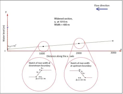
For the implementation of the widening case in WAQUA, a grid is also used of = 1 m and = 1 m (see Figure 17). The original width of the river is 360 m, which is between 0 m and 1000 m and in-between 2000 m and 3000 m along the river.

Figure 17; Grid used in 2DV calculation of the widening measure

Furthermore, the bed level is modeled uniformly in lateral direction, with a slope of 1 m / 10 km in longitudinal (see figure 18).

Figure 18; Bed level for widening case

For the computation with the constant eddy viscosity estimated with Madsen et al (1988), a value of is used since the flow velocity in the river is approximately 2 m/s.

Similar to the numerical solutions in the 1D analysis, the water depth is discretized using a Froward Euler scheme, using a staggered grid. For more detailed information about this solution, refer to the technical report of WAQUA (Rijkswaterstaat, 2012).

3.4 Boundary Conditions

(39)

4 Results

4.1 Model configuration I: 1D - Bernoulli

First the result of the deepening measure is shown in Figure 19. The term ̿ [m/s] equals the depth and time averaged flow velocity, zw [m] is the water depth and zb [m] is the bed level. The term ̿ and zh,0

equals the incoming velocity and water depth respectively and zb,0 equals the bed level at x = 0.

Furthermore, the energy is conserved in the domain since no energy is dissipated by sources such as bottom friction or bed slope. It is shown that in this case the decrease of the bed level by 1 m causes the water depth to be 1.0226 meters and therefore an increase in the water level of 2.26 cm.

The increase in water level as the bed level decreases is as expected, since the Froude number in this situation is lower than 1, indicating sub-critical flow. Equation 3.3 shows that when the Froude number is lower than 1, the water depth increases faster than the bed level decreases, indicating that the water level is increasing.

Figure 19; water level of the deepening measure when applying Bernoulli

(40)

The result of the widening measure is shown in figure 20. Instead of a changing bed level, the width changes from 360 m to 400 m. This causes the total water level to increase with 3.76 cm.

Figure 20; water level of the widening measure when applying Bernoulli

This is what is expected from the equation describing the change of the water level as function of the Froude number (see equation 3.8). When the Froude number is smaller than 1,

is positive, but when

the Froude number is larger than 1,

becomes negative. Therefore only in the case of sub critical flow

the water level rises.

Concluding remarks

In this configuration a situation is considered in which the friction term is neglected. Both at the downstream side of the deepening and widening measure, the water level increases at the location where the river profile expands or the flow decelerates, and it decreases to its original water level at the location where the river profile is constricted or accelerates. This is only the case for sub-critical flow; the opposite occurs for super-critical.

(41)

4.2 Model configuration II: 2D – Bélanger

4.2.1 Deepening measure

Analytical solution

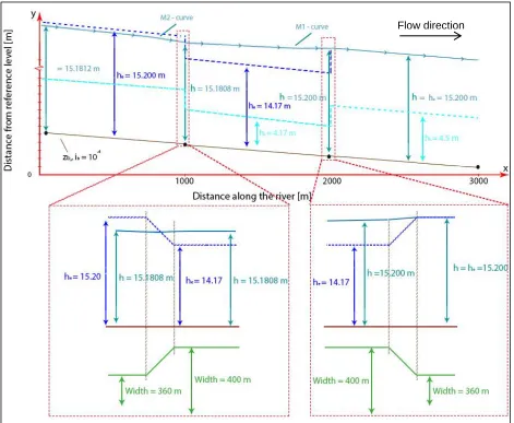
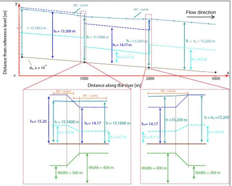
The result of the 1D analysis is shown in Figure 21. It is described mathematically according to the analytical solution of Bresse. In this situation, the equilibrium depth is equal to 15.200 m. Since there is subcritical flow, the lowering of the bed has no effect downstream of the intervention and the water depth at the section x = 2000 m to x = 3000 m is equal to the equilibrium depth. At the section in between x = 1000 m and x = 2000 m, the bed level is lowered by 1 m. The equilibrium depth remains the same (he =

15.200 m), however, due to the lowering of the bed, the water depth at point x = 2000 m is 16.200 meter. The water depth develops towards its equilibrium depth when going further upstream to point x = 1000 m. The ‘half adaption length’ at this section is ca. 40 km and very large compared to the 1000 m meter over which the bed is decreased. Therefore the lowering of the bed by 1 meter over 1000 meter length causes the water level to lower by only 18 mm. At the section x = 1000 m to x = 0 m, the bed level is increased with 1 meter again. The depth right after x = 1000 m is 16.182 meters, however, due to the increase of the bed of 1 meter the depth at point x = 1000 m is 15.182 meters. When going further upstream, the water depth develops back to the equilibrium depth. The half adaption length of the section in between x = 0 m and x = 1000 m is ca. 36 km. This is again very large compared to the 1000 m section that is considered, and the water is increased over this section by only 1 mm. The water depth at x = 0 m is thus 15.183 meter.

In the whole domain, he > hc, so there is a mild slope. At section x = 0 to x = 1000 m, hc < h < he, therefore

there is a M2 curve at this section. At section x = 1000 m to x = 2000 m, he > h and hc <h. Therefore at

this section a M1 – curve occurs (de Vries, 1985).

Figure 21; Solution of Bélanger according to approximation of Bresse applied to the deepening measure

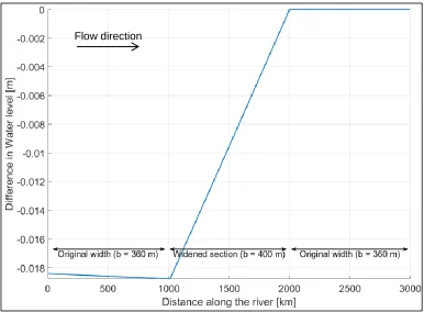
Furthermore, in Figure 22 the difference in water level is shown between the situation with intervention and the situation without intervention. For the situation without intervention, the water depth is equal to the equilibrium depth over the whole domain, i.e. h = he = 15.2 m. This Figure shows the water level as

depicted in Figure 21 minus the water level of the reference situation. It can be seen that the water level is lowered by ca. 18 mm at x = 1000 m and by 17 mm at x = 0.

(42)

Figure 22; Difference between situation with and without intervention

Numerical solution

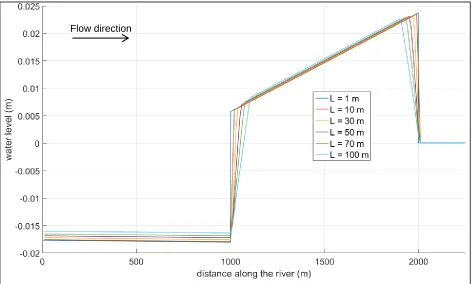
The result of the numerical solution can be seen in Figure 23, showing that in between x = 3000 m to x = 2000 m the water depth is the same as the equilibrium depth, i.e. h = 15.200 m. However, from x = 1990 to x = 2000, the water level increases in upstream direction. At this region, the bed level is negative, and since

√ , he becomes undefined. Due to the negative slope and hc < h, the water level decreases

according to an A2 curve. From x = 1990 m to x = 1010 m, the water level decreases according to a M1 curve, since h > he. From x = 1010 m to x = 1000 m, due to the sudden increase of the slope, the

equilibrium depth drops significantly from 15.2 m to 1.9 m. Therefore hc > he so the water level to drops

according to a S1 curve. From x = 1000 m to x = 0 m the equilibrium depth is 15.2 m and the water level increases towards the equilibrium depth according to a M2 curve as h < he.

(43)

Figure 23; Detailed figure of the situation with deepened bed with using the numerical solution of Bélanger

In Figure 24 the difference between the situation without any intervention and the result of the numerical solution is conveyed. At section x = 2000 m to x = 3000 m, there is no difference, being downstream of the intervention. At the location of the intervention, i.e. at x = 1000 m to x = 2000 m, the water level has increased over the entire section compared to the original. In this model, the maximum increase of the water level is 23.6 mm at x = 2000 m. At x = 0 to x = 1000 m, the water level is decreased over the entire section. The maximum decrease is 18 mm at x = 1000 m and the decrease at x = 0 m is 17 mm.

Flow direction

Analysis of flow processes at the downstream side of various river measures using 1D and 2D flow models

Anal

ys

i

s

of

ow

pr

oces

s

es

at

t

he

down-s

t

r

eam

s

i

de

of

var

i

ous

r

i

ver

meas

ur

es

us

i

ng

1D-

and

2D ow

model

s

Mas

t

er

Thes

i

s

Mi

chi

el

Cl

ement

s

Analysis of flow process at the

downstream side of various

river measures using 1D- and

2D flow models

Master Thesis Michiel Clements

August 2016

Graduation Committee:

Ir. R.P. van Denderen

University of Twente

Dr. Ir. J.S. Ribberink

University of Twente

Dr. A.P. Tuijnder

Arcadis

Preface

Summary

Table of contents

1 Introduction

1.1 Background

1.2 The downstream peak

1.3 Policy regarding the downstream peak

1.4 Research motivation and questions

1.5 Research approach

1.6 Outline report

2 Flow Theory

2.1 Navier-Stokes equations

2.2 Reynolds averaged Navier-Stokes equations

2.3 Shallow water flow: the assumption of shallowness and steadiness

2.4 Model configuration I: 1D - Bernoulli

2.5 Model Configuration II: 1D - Bélanger