http://wrap.warwick.ac.uk
Original citation:
Reyes Aldasoro, Constantino Carlos and Bhalerao, Abhir. (2007) Volumetric texture segmentation by discriminant feature selection and multiresolution classification. IEEE Transactions on Medical Imaging, Volume 26 (Number 1). pp. 1-14. ISSN 0278-0062
Permanent WRAP url:
http://wrap.warwick.ac.uk/32533
Copyright and reuse:
The Warwick Research Archive Portal (WRAP) makes this work by researchers of the University of Warwick available open access under the following conditions. Copyright © and all moral rights to the version of the paper presented here belong to the individual author(s) and/or other copyright owners. To the extent reasonable and practicable the material made available in WRAP has been checked for eligibility before being made available.
Copies of full items can be used for personal research or study, educational, or not-for profit purposes without prior permission or charge. Provided that the authors, title and full bibliographic details are credited, a hyperlink and/or URL is given for the original metadata page and the content is not changed in any way.
Publisher’s statement:
“© 2007 IEEE. Personal use of this material is permitted. Permission from IEEE must be obtained for all other uses, in any current or future media, including reprinting
/republishing this material for advertising or promotional purposes, creating new collective works, for resale or redistribution to servers or lists, or reuse of any copyrighted component of this work in other works.”
A note on versions:
The version presented here may differ from the published version or, version of record, if you wish to cite this item you are advised to consult the publisher’s version. Please see the ‘permanent WRAP url’ above for details on accessing the published version and note that access may require a subscription.
Volumetric Texture Segmentation by Discriminant
Feature Selection and Multiresolution Classification
Constantino Carlos Reyes-Aldasoro∗ and Abhir Bhalerao, Member, IEEE
Abstract
In this paper a Multiresolution Volumetric Texture Segmentation(M-VTS) algorithm is presented. The method extracts textural measurements from the Fourier domain of the data via subband filtering using an Orientation Pyramid [1]. A novelBhattacharyya space, based on the Bhattacharyya distance, is proposed for selecting the most discriminant measurements and producing a compact feature space. An oct tree is built of the multivariate features space and a chosen level at a lower spatial resolution is first classified. The classified voxel labels are then projected to lower levels of the tree where a boundary refinement procedure is performed with a 3D equivalent of butterfly filters. The algorithm was tested in 3D with artificial data and three Magnetic Resonance Imaging sets of human knees with encouraging results. The regions segmented from the knees correspond to anatomical structures that can be used as a starting point for other measurements such as cartilage extraction.
Keywords: Volumetric texture, Filtering, Multiresolution, Texture Segmentation
I. INTRODUCTION
The labeling of tissues in medical imagery such as Magnetic Resonance Imaging (MRI) has rightly received a great deal of attention over the past decade. Much of this work has concentrated on the classification of tissues by grey level contrast alone. For example, the problem of grey-matter white-matter labeling in central nervous system (CNS) images like MRI head-neck studies has been addressed by supervised statistical classification methods, notably EM-MRF [2]. The success of these methods is partly as a result of incorporating MR bias-field correction into the classification process [3], which can be regarded as extending the image model from a piece-wise constant plus noise model to include a slowly varying additive or multiplicative intensity bias. Another reason why first-order statistics have been adequate in many instances is that the MR imaging sequence can be adapted or tuned to increase contrast in the tissues of interest. For example, a T2 weighted sequence is ideal for highlighting cartilage in MR orthopedic images, or the use of iodinated contrast agents for tumors and vasculature. Also, multimodal image registration enables a number of separately acquired images to be effectively fused to create a multichannel or multispectral image as input to a classifier. Other than bias field artifact, the ‘noise’ in the image model incorporates variation of the voxel grey-levels due to the texturalqualities of the imaged tissues and, with the ever increasing resolution of MR scanners, it seems expedient to model and use this variation, rather than subsuming it into the image noise.
The machine vision community has extensively researched the description and classification of 2D textures, but even if the concept of image texture is intuitively obvious to us, it can been difficult to provide a satisfactory definition. Texture relates to the surface or structure of an object and depends on the relation of contiguous elements and may be characterized by granularity or roughness, principal orientation and periodicity (normally associated with man-made textures such as woven cloth). Early work of Haralick [4] is a standard reference for statistical and structural approaches for texture description. Other approaches include contextual methods like Markov Random Fields as used by Cross and Jain [5], and fractal geometry methods by Keller [6]. Texture features derived from the grey level co-occurrence matrix (GLCM) calculate the joint statistics of grey-levels of pairs of pixels at varying distances. Unfortunately, for addimensional image of sizeN makes the descriptor have a complexity ofO(NdM2), where M is the number of grey levels. This will be prohibitively high for d= 3 and an image sizes of N = 512
quantized to, say,M = 64grey levels. For these reasons and to capture the spatial-frequency variation of textures, filtering methods akin to Gabor decomposition [7] and joint spatial/spatial-frequency representations like wavelet transforms [8] have been reported. Randen and Husøy [9] have shown that co-occurrence measures are outperformed
by such filtering techniques. The dependence of texture on resolution or scale has been recognized and exploited by workers which has led to the use of multiresolution representations such as the Gabor decomposition and the wavelet transform [8] [10]. Here, we use the Wilson-Spann subband filtering approach [11], which is similar to the Gabor filtering and has been proposed as a ‘complex’ wavelet transform [12].
The importance of texture in MRI has been the focus of some researchers, notably Lerksi [13] and Schad [14], and a COST European group was established for this purpose [15]. Texture analysis has been used with mixed success in MRI, such as for detection of microcalcification in breast imaging [16] and for knee segmentation [17], and in CNS imaging to detect macroscopic lesions and microscopic abnormalities such as for quantifying contralateral differences in epilepsy subjects [18], to aid the automatic delineation of cerebellar volumes [19], to estimate effects of age and gender in brain asymmetry [20], and to characterize spinal cord pathology in Multiple Sclerosis [21]. Most of the reported work, however, has employed solely 2D measures, again based on GLCM. Furthermore, feature selection may be neglected or done in an ad-hoc way, with no regard to training data which are usually available.
Since not all features derived from subband filtering or statistical feature extraction scheme have the same discrimination power, it is prudent to perform some form of feature selection. When a large number of features are input to a classifier, some may be irrelevant while others will be redundant - which will at best increase the complexity of the task, and at worst hinder the classification by increasing the inter-class variability. Subspace methods like PCA are traditionally used for feature selection where the feature space is transformed to a set of independent and orthogonal axes which can be ranked by the extent of variation given by the associated eigenvalues. Fisher’s linear discriminant analysis (LDA), on the other hand, finds the feature space mapping which maximizes the ratio of between-class to within-class variation jointly for each feature (dimension) [22] given a set of training data. PCA can be further applied to find a compact subspace to reduce the feature dimensionality. However, while these methods are optimal and effective, they still require the computation of all the features.
We propose a supervised feature selection methodology based on the discrimination power or relevance of the individual features taken independently; the ultimate goal is to select a subset of discriminant features. In order to obtain a quantitative measure of how separableare two classes given a feature, a distance measure is required. We have studied a number measures (Bhattacharyya, Euclidean, Kullback-Leibler [23], Fisher) and have empirically shown that the Bhattacharyya distance works best on a range of textures [24]. This is developed into the concept of a feature selection space in which discrimination decisions can be made. A multiresolution classification scheme is then developed which operates on the joint data-feature space within an oct-tree structure. This benefits both the efficiency of the computation and ensures only the certain labelings at a given resolution are propagated to the next. Interfaces between regions (planes), where the label decisions are uncertain, are smoothed by the use of 3D ‘butterfly’ filters which focus the inter-class labels to likely candidate labels [25].
The paper is organized as follows. In Section II, we provide a definition of volumetric texture. In Section III, a measurement extraction technique based on a multiresolution subband filtering is presented. Section IV introduces a Bhattacharyya space for feature selection and a multiresolution classification algorithm is described in Section V. An extension of the so-called butterfly filters to 3D is used for boundary refinement. The relationship of our classifier with traditional Markov Random Fields is also sketched out. Experimental results on 2D and 3D data are presented and discussed in Section VI, and Section VII draws some final conclusions.
II. VOLUMETRIC TEXTURE
(a) (b) (c)
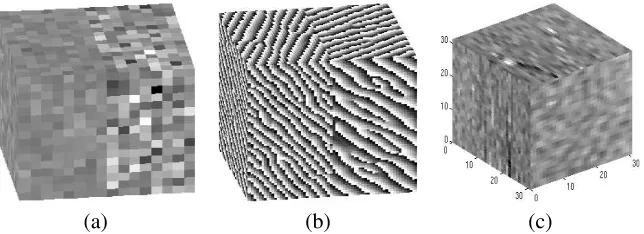
Fig. 1. Volumetric texture examples: (a) A cube divided into two regions with Gaussian noise, (b) A cube divided into two regions with oriented patterns of different frequencies and orientations, (c) A sample of muscle from MRI.
Throughout this work, we consider volumetric data,V, represented as a function that assigns a gray tone to each triplet of co-ordinates:
V :Lr×Lc×Ld→G, (1)
where Lr = {1,2, . . . , r, . . . , Nr}, Lc = {1,2, . . . , c, . . . , Nc} and Ld = {1,2, . . . , d, . . . , Nd} are the spatial
domains of the data of dimension Nr ×Nc ×Nd (using subscripts (r, c, d) for row, columns and slices) and G={1,2, . . . , g, . . . Ng} is the set of Ng gray levels.
III. FEATUREEXTRACTION: SUB-BAND FILTERING USING ANORIENTATIONPYRAMID(OP)
Certain characteristics of signals in the spatial domain such as periodicity are quite distinctive in the frequency or Fourier domain. If the data contain textures that vary in orientation and frequency, then certain filter subbands will contain more energy than others. The principle of subband filtering can equally be applied to images or volumetric data.
Wilson and Spann [1] proposed a set of operations that subdivide the frequency domain of an image into smaller regions by the use of two operators quadrant andcenter-surround. By combining these operators, it is possible to construct different tessellations of the space, one of which is the Orientation Pyramid (OP) (Figure 2). A band-limited filter based on truncated Gaussians is used to approximate the finite prolate spheroidal sequences used in [1]. The filters are real functions which cover the Fourier half-plane. Since the Fourier transform of a real signal is symmetric, it is only necessary to use a half-plane or a half-volume to measure subband energies. A description of the subband filtering with the OP method follows.
Any given volume V whose centered Fourier transform is Vω =F[V] can be subdivided into a set of i
non-overlapping regions Lir×Lic×Ldi of dimensions Nri, Nci, Ndi. In 2D, the OP tessellation involves a set of 7 filters, one for the low pass region and six for the high pass (Figure 2 (a)). In 3D, the tessellation will consist of 28 filters for the high pass region and one for the low pass (Figure 2 (c)). The i-th filter Fωi in the Fourier domain (Fωi =F[Fi]) is related to the i-th subdivision of the frequency domain as:
Fωi :
Lir×Lic×Ldi → Ga(µi,Σi),
(Lir×Lic×Lid)c → 0
∀i∈OP, (2)
where Ga describes a Gaussian function, with parametersµi, the center of the region i, and Σi is the co-variance matrix that will provide a cut-off of 0.5 at the limit of the band (see Figure 2 (d,e) for 2D filters). The measurement space S in its frequency and spatial domains is then defined as:
Swi(ρ, κ, δ) = Fωi(ρ, κ, δ) Vω(ρ, κ, δ)
Si = |F−1[Sωi]|, (3)
where(ρ, κ, δ)are the co-ordinates in the Fourier domain. At the next level, the coordinates(L1r(1)×L1c(1)×L1d(1))
will become(Lr(2)×Lc(2)×Ld(2))with dimensionsNr(2) = Nr2(1), Nc(2) = Nc2(1), Nd(2) = Nd2(1). It is assumed
thatNr(1) = 2a, Nc(1) = 2b, Nd(1) = 2c so that the results of the divisions are always integer values. To illustrate
1 2
3 4
7 6
5 5 6
7 9
10 11 12 13 14 4 3 2 8 !!!!!! !!!!!! !!!!!! !!!!!! """ """ """ """ ### ### ### ### $$$$ $$$$ $$$$ %%%% %%%% %%%% &&&&&& &&&&&& &&&&&& &&&&&& '''''' '''''' '''''' '''''' ((( ((( ((( ((( ))) ))) ))) ))) ** ** ** ** ++ ++ ++ ++ ,,,,,, ,,,,,, ,,,,,, ,,,,,, ---... ... ... ////// ////// ////// 00000 00000 11111 11111 2222 2222 3333 3333 444 444 444 444 555 555 555 555 66666 66666 66666 77777 77777 77777 8888 8888 9999 9999 :: :: :: :: ;; ;; ;; ;; <<<< <<<< <<<< ==== ==== ==== >>>>> >>>>> >>>>> >>>>> ????? ????? ????? ????? @@@ @@@ @@@ @@@ AAA AAA AAA AAA BBBB BBBB BBBB CCCC CCCC CCCC DDDDD DDDDD DDDDD DDDDD EEEEE EEEEE EEEEE EEEEE FFF FFF FFF FFF GGG GGG GGG GGG HHHH HHHH HHHH IIII IIII IIII JJJJJ JJJJJ JJJJJ KKKKK KKKKK KKKKK LLL LLL LLL LLL MMM MMM MMM MMM NNNN NNNN NNNN OOOO OOOO OOOO PP PP PP PP QQ QQ QQ QQ RRRRRR RRRRRR RRRRRR SSSSSS SSSSSS SSSSSS TTTTTT TTTTTT TTTTTT UUUUUU UUUUUU UUUUUU VVVV VVVV WWWW WWWW XXXXXX XXXXXX XXXXXX YYYYYY YYYYYY YYYYYY ZZ ZZ ZZ ZZ [[ [[ [[ [[ \\\\ \\\\ \\\\ ]]]] ]]]] ]]]] ^^^^^ ^^^^^ ^^^^^ ^^^^^ _____ _____ _____ _____ ````` ````` ````` ````` aaaaa aaaaa aaaaa aaaaa bbbb bbbb bbbb cccc cccc cccc ddd ddd ddd ddd eee eee eee eee fffff fffff fffff fffff ggggg ggggg ggggg ggggg hhh hhh hhh hhh iii iii iii iii jjj jjj jjj jjj kkk kkk kkk kkk llll llll mmmm mmmm nn nn nn nn oo oo oo oo pppppp pppppp pppppp qqqqqq qqqqqq qqqqqq rrrr rrrr rrrr ssss ssss ssss ttttt ttttt ttttt ttttt uuuuu uuuuu uuuuu uuuuu vvv vvv vvv vvv www www www www xxxx xxxx xxxx yyyy yyyy yyyy zzzzz zzzzz zzzzz zzzzz {{{{{ {{{{{ {{{{{ {{{{{ ||| ||| ||| ||| }}} }}} }}} }}} ~~~~ ~~~~ ~~~~ ¡¡¡ ¡¡¡ ¡¡¡ ¡¡¡ ¢¢¢¢ ¢¢¢¢ ¢¢¢¢ ££££ ££££ ££££ ¤¤¤ ¤¤¤ ¤¤¤ ¤¤¤ ¥¥¥ ¥¥¥ ¥¥¥ ¥¥¥ ¦¦¦¦¦¦ ¦¦¦¦¦¦ ¦¦¦¦¦¦ §§§§§§ §§§§§§ §§§§§§ ¨¨¨¨ ¨¨¨¨ ¨¨¨¨ ©©©© ©©©© ©©©© ªªªªªªªªª ªªªªªªªªª ªªªªªªªªª ªªªªªªªªª ««««««««« ««««««««« ««««««««« ««««««««« ¬¬¬¬¬¬¬¬¬¬¬¬¬ ¬¬¬¬¬¬¬¬¬¬¬¬¬ ¬¬¬¬¬¬¬¬¬¬¬¬¬ ¬¬¬¬¬¬¬¬¬¬¬¬¬ ¬¬¬¬¬¬¬¬¬¬¬¬¬ ¬¬¬¬¬¬¬¬¬¬¬¬¬ ®®®® ®®®® ®®®® ®®®® ®®®® ®®®® ®®®® ®®®® ®®®® ¯¯¯¯ ¯¯¯¯ ¯¯¯¯ ¯¯¯¯ ¯¯¯¯ ¯¯¯¯ ¯¯¯¯ ¯¯¯¯ ¯¯¯¯
(a) (b) (c)
[image:5.612.121.494.65.267.2](d) (e)
Fig. 2. (a-c) 2D and 3D Orientation Pyramid (OP) tessellation: (a) 2D order 1, (b) 2D order 2, (c) 3D order 1. (d,e) Band-limited 2D Gaussian filter: (d) Frequency domain|Fωi|, (e) Magnitude of spatial domain|Fi|.
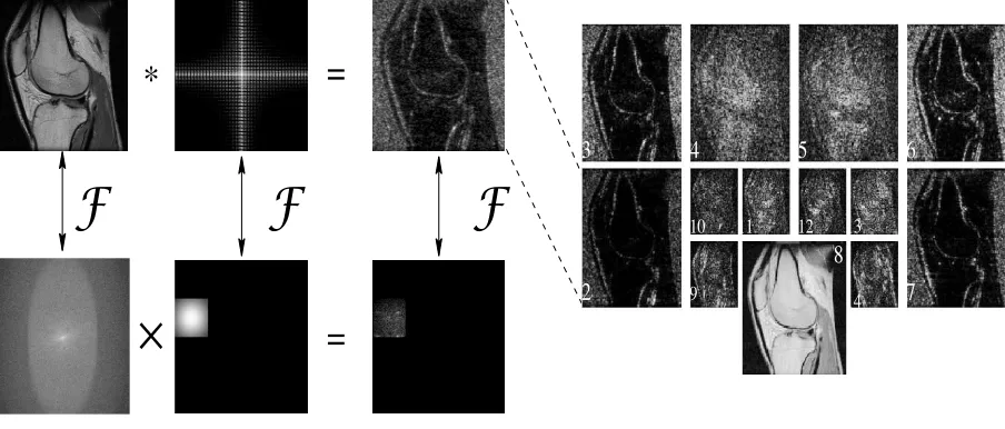
Fig. 3. A graphical example of subband filtering. The top row corresponds to the spatial domain and the bottom row the Fourier domain. Once slice from a knee MRI data set is filtered with a subband filter with a particular frequency and orientation by a product in the Fourier domain, which is equivalent to a convolution in the spatial domain. The filtered image becomes one measurement of the spaceS2 in this example.
IV. FEATURE SELECTIONUSING THE BHATTACHARYYA SPACE
The subband filtering of the textured data produces a series of measurements that belong to ameasurement space
S. Whether this space corresponds to the results of filters, features of the co-occurrence matrix or wavelets, not all the dimensions will contribute to the discrimination of the different textures that compose the original data. Besides the discrimination power that some measurements have, there is an issue of complexity related to the number of measurements used. Each extra texture feature may enrich the measurement space but will also further burden any subsequent classifier. Another advantage of selecting a subset of the space is that it can provide a better understanding of the underlying process that generated the data [31].
[image:5.612.86.538.311.504.2]evaluation functions – is at the same time its weakness, since the classification process can be slow.
The Bhattacharyya space is presented as a method that provides a ranking for the measurements based on the discrimination of a set of training data. This ranking process provides a single evaluation route and, therefore, the number of classifications which remain for every new feature is significantly reduced. In order to obtain a quantitative measure of classseparability, a distance measure is required. With the assumption about the underlying distributions, a probabilistic distance can be easily extracted from some parameters of the data. Kailath [34] compared the Bhattacharyya distance and the Divergence (Kullback-Leibler), and observed that Bhattacharyya distance yields better results in some cases while in other cases they are equivalent. A recent study [35] considered a number of measures: Bhattacharyya, Euclidean, Kullback-Leibler, Fisher, for texture discrimination and concluded that the Bhattacharyya distance is the most effective texture discriminant for subband filtering schemes.
In its simplest formulation, the Bhattacharyya distance [36] between two classes can be calculated from the variance and mean of each class in the following way:
DB(k1, k2) =
1
4ln
1 4(
σk2
1
σ2
k2
+σ
2
k2
σ2
k1 + 2)
!
+1
4
(µk1−µk2)
2
σ2
k1+σ
2
k2
!
, (4)
where DB(k1, k2) is the Bhattacharyya distance between two different training classes k1 and k2, and µk1, σk1
correspond to the mean and variance of each one.
The Mahalanobis distance is a particular case of the Bhattacharyya distance, when the variances of the two classes are equal; this eliminates the first term of the distance that depends solely on the variances of the distribution. If the variances are equal this term will be zero, and grows as the variances differ. The second term, on the other hand, will be zero if the means are equal and is inversely proportional to the variances.
The Bhattacharyya space,B(i, p), is defined on the measurement space S as:
Lp×Li;B(i, p) :Lp×Li →DB(Ski1, Ski2). (5)
where each class pair,p, between classesk1, k2at measurementiwill have a Bhattacharyya distanceDB(Ski1, Ski2),
and will produce a Bhattacharyya space of dimensions Np = (Nk
2) and Ni = 7o :Np×Ni (2D). The domains of
the Bhattacharyya space are Li ={1,2, . . .7o} and Lp ={(1,2),(1,3), . . .(k1, k2), . . .(Nk−1, Nk)} where o is
the order of the OP. In the volumetric case, Lp remains the same (since it depends on the classes only),Ni = 29o
and Li ={1,2, . . .29o}.
The marginal distributions ofB(i, p) are
BI(i) =
Np X
p=1
B(i, p) =
Np X
p=1
DB(Ski1, Ski2), i= 1, . . . , Ni, (6)
BP(p) =
Ni X
i=1
B(i, p) =
Ni X
i=1
DB(Ski1, Ski2), p= 1, . . . , Np. (7)
The marginal over the class pairs,BI(i)sums the Bhattacharyya distances of every pair of a certain feature and thus
will indicate how discriminant a certain subband OP filter is over the whole combination of class pairs. Whereas the marginal BP(p) sums the Bhattacharyya distances for a particular pair of classes over the whole measurement
space and reveals the discrimination potential of particular pairs of classes when multiple classes are present. To visualize the previous distribution, the Bhattacharyya space and its two marginal distributions were obtained for a natural texture image with 16 classes (figure 4(a)). Figure 4(c) shows the Bhattacharyya space forS of order5, and (d) marginalBI(i). These graphs yield useful information toward the selection of the features for classification.
A certain periodicity is revealed in the measurement space;B1,7,14,21,28 have the lowest values (this is clearer in the marginal BI(i)). The feature measurements 1, 7, 14, 21, and 28 correspond to low pass filters of the 2D OP. Since
the textures that make up this mosaic have been deliberately histogram equalized, the low pass features provide the lowest discrimination power. The most discriminant features for the training data presented are S19,18,11,... which correspond to the order statistic B(I)(i) ={BI(1), BI(2), . . . BI(7o)}whereBI(1)≤BI(2)≤. . .. In other words,
(a) (b)
(c) 5 10 15 20 25 30 35
20 40 60 80 100 120
0.5 1 1.5 2
Measurement Space Class Pairs
Bhattacharyya distance
(d) 5 10 15 20 25 30 35
5 10 15 20 25
Measurement Space
[image:7.612.164.446.66.415.2]Bhattacharyya distance
Fig. 4. (a) 16-class natural texture mosaic (image f from Randen [37]). (b) Classification result using BS selected features. Average classification error is 16.5%. (c) The Bhattacharyya spaceB for a measurement spaceS of order 5 from the 16-texture image. (d) Marginal BI(i), the indexMeasurement Spacecorresponds to spaceS.
is shown in figure 4(b) and has an average label error 16.5% which compares favorably with other methods e.g. Randen reports an error of 34.7% on this image using a quadrature-mirror subband filtering and a vector quantization for the classifier [37]. It is important to mention two aspects of this selection process: the Bhattacharyya space is constructed on training data and the individual Bhattacharyya distances are calculated between pairs of classes. Therefore, there is no guarantee that the feature selected will always improve the classification of the whole data space, the features selected could be mutually redundant or may only improve the classification for a pair of classes but not the overall classification [38]. Thus the conjecture to be tested then is whether the classification can be improved in abest-first, sequential selection defined by the Bhattacharyya space order statistics. The natural textures image was classified with several sequential selection strategies:
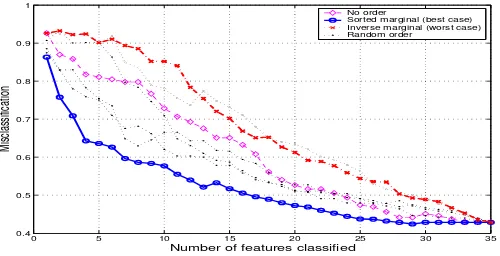
• Following the unsorted order of the measurement space: S1, S2, S3 etc. • Following the marginal BI(i) in decreasing order: S19, S18,S11 etc.
• Following the marginal BI(i) in increasing order: S28, S21, S15 etc. (The converse conjecture is that the
reverse order should provide the worst path for the classification.)
• Three random permutations.
The sequential misclassification results of the previous strategies are presented in Figure 5 where the advantage of the route provided by the B(I) can be seen. If extra time can be afforded, then the training data can be used with a
more elaborate feature selection strategy; various forward and backward optimizations are possible (see [38]). Our experiments on 2D texture mosaics, however, have not shown a significant benefit by these methods in the final classification error over the sub-optimal best-first approach used here [39], and we have demonstrated superior performance over other techniques: Local Binary Pattern (LBP) and the p8 methods presented by Ojala [40]; and
0 5 10 15 20 25 30 35 0.4
0.5 0.6 0.7 0.8 0.9 1
Number of features classified
Misclassification
No order
[image:8.612.184.434.68.196.2]Sorted marginal (best case) Inverse marginal (worst case) Random order
Fig. 5. Misclassification error for the sequential inclusion of features to the classifier for the 16-class natural textures image (figure 4(a)). The route provided by the ordered marginalsB(I)(i)yields the best classification strategy.
Another solution that is provided by the order statistics of the Bhattacharyya space marginal is the option to select a predetermined number of features as thereduced setor sub-space used for classification. This can be particularly useful in cases where it can be computationally expensive to calculate the entire measurement space. Then, based on the training data, only a few measurements need to be generated based on the first n features of the B.
V. MULTIRESOLUTIONCLASSIFICATION
This section presents a new multiresolution algorithm, Multiresolution-Volumetric Texture Segmentation (M-VTS). The multiresolution procedure consists of three main stages: the process of climbing the levels or stages of a pyramid or tree, a decision or classification at the highest level is performed, and the process of descending from the highest level down to the original resolution. Based on the decision-directed approach of Wilson and Spann [1], we replace the contextual boundary-refinement step at each scale with a steerable-filter based on butterfly neighborhoods [25]. This is a satisfactory compromise over the use of a multiresolution MRF to gain a notion of contextual label smoothing but avoids the need to model and estimate a complicated set of boundary priors over 3D neighborhoods [42].
Smoothing the measurement space can improve the classification results; many isolated elements disappear and regions are more uniform. But a new problem arises with smoothing, especially at the boundaries between textures. When the measurement values of elements that belong to the same class are averaged, it is expected that they will tend to the class prototype, but if the elements belong to different classes, the smoothing can place them in a different class altogether. It would be ideal to smooth selectively depending on the distance to the boundaries. Of course, the class boundaries need then to be known. A compromise has to be reached between the intra-class smoothing and the class boundary estimation. A solution to this problem is to apply a multiresolution procedure of smoothing several levels with a pyramid before estimating the boundaries at the highest level and applying a boundary refinement algorithm in the descent to the highest resolution.
A. Smoothing the Measurement Space
The climbing stage represents the decrease in resolution of the data by means of averaging a set of neighbors on one level (children elements or nodes) up to a parent element on the upper level. Two common climbing methods are the Gaussian Pyramid [43] and the Quad tree ([44], [45], [46]). In our implementation we used the quad tree structure which, in 3D, becomes an oct tree (OT). The decrease in resolution correspondingly reduces the uncertainty in the elements’ values since they tend toward their mean. In contrast, the positional uncertainty increases at each level [1].
The measurement spaceS constitutes the lowest level of the tree. For each measurementSi of the space, a OT
is constructed. To climb a level in the OT, a REDU CE operation is performed [43]:
(Si)L=REDU CE(Si)L−1, (8)
B. Classification
At the highest level, the new reduced space can be classified. Partitioning of the measurement space can be considered as a mapping operator
λ:S→ {1,2, . . . , Nk}, (9)
where the clusters or classes are λ−1(1), λ−1(2), ... , and these are unknown. Then, for every element x ∈ S,
λa will be an estimator for λ where, for every class, there is a point {a1, a2, . . .} ∈ S such that these points
define hyperplanes perpendicular to the chords connecting them, and split the space into regions {R1, R2, . . .}.
These regions define the mapping function λa :S → {1,2. . . , Nk} by λa(x) =K if x ∈RK, K = 1,2, ..., NK.
This partitioning should minimize the Euclidean distance from the elements of the space to the points a, expressed by [47]:
ρ(a1, a2, . . .) =
X
x∈(Lr×Lc×Ld)
min
1≤j≤Nk
||S(x)−aj||. (10)
The measure of closeness of the estimator λa to λdefines a misclassification error by [λa] =P(λa(x)6=λ(x)), and P(λa(S) 6= λ(S)) for an arbitrary point x ∈ S in the space. If the values of the points ak are known, or
there is a way of estimating these from training data, the classification procedure is supervised, otherwise it is unsupervised. For this work, the points in the measurement space ak were obtained by filtering separate training
data with the OP. Once the measurement space S is calculated for every training image, the average can be used as an estimate of the mean of the class: ˆak and equation 10 can be minimized by an iterative method such nearest
neighbor (NN) clustering. In the experiments presented below, where supervised classification was required we used a NN approach.
C. Boundary Refinement
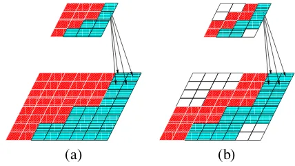
To regain full spatial resolution at the lowest level of the tree, the classification at the higher level has to be propagated downward. The propagation implies that every parent bequeaths: (a) its class value to 8 children and; (b) the attribute of being or not being in a boundary (figure 6). Interaction between neighbors can reduce the uncertainty in spatial position that is inherited from the parent node. This process is known as spatial restoration and boundary refinement, which is repeated at every stage until the bottom of the tree or pyramid is reached. We
[image:9.612.199.413.466.587.2]!!!! !!!! !!!! """" """" """" #### #### #### $$$$ $$$$ $$$$ %%% %%% %%% &&& &&& &&& ''' ''' ''' ((( ((( ((( ))) ))) ))) *** *** *** +++ +++ +++ ,,, ,,, ,,, ---... ... ... /// /// /// 000 000 000 1111 1111 1111 2222 2222 2222 3333 3333 3333 4444 4444 4444 555 555 555 666 666 666 777 777 777 888 888 888 999 999 999 ::: ::: ::: ;;; ;;; ;;; <<< <<< <<< === === === >>> >>> >>> ???? ???? ???? @@@@ @@@@ @@@@ AAAA AAAA AAAA AAAA BBBB BBBB BBBB CCCC CCCC CCCC CCCC DDDD DDDD DDDD EEEE EEEE EEEE EEEE FFFF FFFF FFFF GGGG GGGG GGGG GGGG HHHH HHHH HHHH IIII IIII IIII IIII JJJJ JJJJ JJJJ KKK KKK KKK KKK LLL LLL LLL MMMM MMMM MMMM MMMM NNNN NNNN NNNN OOOO OOOO OOOO OOOO PPPP PPPP PPPP QQQQ QQQQ QQQQ QQQQ RRRR RRRR RRRR SSSS SSSS SSSS SSSS TTTT TTTT TTTT UUUU UUUU UUUU UUUU VVVV VVVV VVVV WWWW WWWW WWWW WWWW XXXX XXXX XXXX YYYY YYYY YYYY YYYY ZZZZ ZZZZ ZZZZ [[[ [[[ [[[ [[[ \\\ \\\ \\\ ]]]] ]]]] ]]]] ]]]] ^^^^ ^^^^ ^^^^ ____ ____ ____ ____ ```` ```` ```` aaa aaa aaa bbb bbb bbb ccc ccc ccc ddd ddd ddd eeee eeee eeee ffff ffff ffff gggg gggg gggg hhhh hhhh hhhh iiii iiii iiii iiii jjjj jjjj jjjj kkk kkk kkk kkk lll lll lll mmm mmm mmm mmm nnn nnn nnn oooo oooo oooo oooo pppp pppp pppp qqq qqq qqq qqq rrr rrr rrr ssss ssss ssss ssss tttt tttt tttt uuuu uuuu uuuu uuuu vvvv vvvv vvvv www www www www xxx xxx xxx yyy yyy yyy yyy zzz zzz zzz {{{{ {{{{ {{{{ {{{{ |||| |||| |||| }}}} }}}} }}}} }}}} ~~~~ ~~~~ ~~~~ !!!! !!!! !!!! """" """" """" #### #### #### $$$$ $$$$ $$$$ %%%% %%%% %%%% &&&& &&&& &&&& '''' '''' '''' (((( (((( (((( )))) )))) )))) **** **** **** ++++ ++++ ++++ ,,,, ,,,, ,,,, ----.... .... .... //// //// //// 0000 0000 0000 1111 1111 1111 1111 2222 2222 2222 3333 3333 3333 3333 4444 4444 4444 5555 5555 5555 5555 6666 6666 6666 7777 7777 7777 7777 8888 8888 8888 9999 9999 9999 9999 :::: :::: :::: ;;;; ;;;; ;;;; ;;;; <<<< <<<< <<<< ==== ==== ==== ==== >>>> >>>> >>>> ???? ???? ???? ???? @@@@ @@@@ @@@@ AAAA AAAA AAAA AAAA BBBB BBBB BBBB CCCC CCCC CCCC CCCC DDDD DDDD DDDD EEEE EEEE EEEE EEEE FFFF FFFF FFFF GGGG GGGG GGGG GGGG HHHH HHHH HHHH IIII IIII IIII IIII JJJJ JJJJ JJJJ KKKK KKKK KKKK KKKK LLLL LLLL LLLL MMM MMM MMM MMM NNN NNN NNN OOOO OOOO OOOO OOOO PPPP PPPP PPPP QQQ QQQ QQQ RRR RRR RRR SSS SSS SSS TTT TTT TTT UUU UUU UUU VVV VVV VVV WWWW WWWW WWWW XXXX XXXX XXXX YYYY YYYY YYYY YYYY ZZZZ ZZZZ ZZZZ [[[[ [[[[ [[[[ [[[[ \\\\ \\\\ \\\\ ]]]] ]]]] ]]]] ]]]] ^^^^ ^^^^ ^^^^ ____ ____ ____ ____ ```` ```` ```` aaaa aaaa aaaa bbbb bbbb bbbb cccc cccc dddd dddd eeee eeee ffff ffff gggg gggg gggg hhhh hhhh hhhh iiii iiii iiii jjjj jjjj jjjj kkkk kkkk kkkk llll llll llll mmmm mmmm mmmm mmmm nnnn nnnn nnnn oooo oooo oooo oooo pppp pppp pppp qqqq qqqq qqqq qqqq rrrr rrrr rrrr ssss ssss ssss tttt tttt tttt uuuu uuuu uuuu uuuu vvvv vvvv vvvv wwww wwww wwww wwww xxxx xxxx xxxx (a) (b)
Fig. 6. Inheritance of labels to child elements: (a) Class inheritance; (b) Boundary inheritance.
tested two methods: a Markov Random Field approach and an extension of the 2D butterfly filters and have shown that pyramidal, volumetric butterfly filters to provide better results.
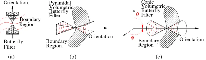
Butterfly filters (BF) [25] are orientation-adaptive filters, that consist of two separate sets orwings with a pivot element between them. It is the pivot elementx= (r, c, d)which is modified as a result of the filtering. Each of the wings will have a roughly triangular shape , which resembles a butterfly (figure 7(a)) and they can be regarded as two separate sets of anisotropic cliques, arranged in a steerable orientation. We propose the extension of these BF
(b) (a)
φ θ
(c)
Volumetric
Volumetric
Region
Boundary Orientation
Filter Butterfly
Boundary Region
Orientation Boundary
Region
Butterfly Orientation
Filter Butterfly
Filter
[image:10.612.137.479.69.169.2]Pyramidal Conic
Fig. 7. (a) 2D Butterfly filter, (b) Pyramidal volumetric butterfly filters, (c) Conic volumetric butterfly filters. Orientation of φ and θ indicated in (c).
by each of the wings are included in the filtering process while the values of the elements along the boundary (which are presumed to have greater uncertainty) and the pivot, x, are not included in the smoothing process. The
BF consists of two sides, with left and right wings: lw/rw, each of which comprisesNw elements:
lw = {lw1, lw2, . . . , lwNw} rw = {rw1, rw2, . . . , rwNw}
lw, rw∈S. (11)
For each wing, an average of the values of the elements in each dimension is calculated:
˜
Slwi (x) = 1
Nw Nw X
q=1
Si(lwq), S˜rwi (x) =
1
Nw Nw X
q=1
Si(rwq). (12)
The actual pivot element x= (r, c, d) value is then combined with the mean values as follows:
˜
Sx−lw = (1−α)S(x) + αS˜lw, (13)
˜
Sx−rw = (1−α)S(x) + αS˜rw. (14)
where α is a scalar gain measure that depends on the dissimilarity of the distribution of the elements that make up the wings:
α= 1
1 +e(5−D), D=
|S˜lw−S˜rw| q
σlw2 +σ2
rw
, (15)
where σ2
lw and σ2rw are the variances of the elements in each butterfly wing. The parameter α acts as weighting
factor of the distance between the distributions covered by the two sides of the butterfly filter, and provides a balance between the current value of the element and a new one calculated from its neighbors. It is interesting to note that this balancing procedure is similar to the update rule of the Kohonen Self Organizing Maps [48].
The distance measure between the updated pivot element and the prototype values of each class determines to which class it is reassigned. Figure 8 shows the process graphically. At the classification stage, the new feature values
˜
Sx−lw,S˜x−rw replace the original feature values of element x. Instead of looking for a class based on λa(S(x)),
the new valuesλa( ˜Sx−lw)/λa( ˜Sx−rw)will determine the class according to its closeness to class prototypes (using
the mapping operator λa from equation 9).
VI. EXPERIMENTALRESULTS
A. 3D Artificial Textures
There are many examples test images available for comparing 2D texture segmentation methods. However, up to the best of the authors’ knowledge, there is not such a database for volumetric texture. We have therefore created a handful of 3D data sets to demonstrate and compare the performance of the presented algorithm and measurement extraction techniques. First, a volumetric set that represents a simple two-class measurement space, each with
32×16×32 elements drawn from Gaussian distributions (Class A:S1 µ1 = 25, σ1= 2,S2 µ2 = 26, σ2= 4, Class
B: S1 µ1 = 27, σ1 = 7, S2 µ2 = 28, σ2 = 7). The two classes together form a 32×32×32×2 space. The data
Feature b
Feature a
Feature b
Feature a Feature a
Feature b
Feature b
Feature a Feature a
Feature b k
(c)
(b)
1−α α
(a)
(d)
(e)
+
x x
+
+
x x
+ 1
[image:11.612.145.465.407.525.2]2
Fig. 8. A feature space view of boundary refinement process with butterfly filters. (a) A boundary elementxwith other elements. (b)x and the two sets of neighboring elements that are comprised by the butterfly wings, all other elements are not relevant at this moment. (c) The weighted average of each wing. (d) Parameterαbalances between the elementxand the average of the wings. (e) New positions are compared with the prototypes (1,2,. . . ,k) of the classes, the class that corresponds to the minimum distance is then assigned tox.
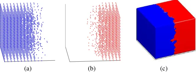
clustered with the Linde-Buzo-Gray vector quantization method (LBG) [49] in a single resolution and then using M-VTS (OT level L = 3). The classification results are presented in Figure 9 as clouds of points for each class for M-VTS. Results are presented in Table I. With M-VTS there are some incorrectly classified voxels close to the boundary, but the general shape of the original data is preserved and its overall error rate is much lower.
The second set is a 64×64×64 volume containing two oriented patterns which have different frequency and orientation (figure 1(b)). The measurement space was extracted and two measurements were manually selected:S1
and S3, and classification was again performed unsupervised for single and multiresolution. Results are presented in Table I.
Again, some voxels near the boundary are misclassified, less than 3%, but the shape (figure 9(c)) is well preserved. The computational complexity was considerably increased in 3D, for the first set the respective times for LBG and M-VTS were 0.1s and 14.9s and for the second set 0.4s and 54.0s.
(a) (b) (c)
Fig. 9. Classification of 3D textures: (a,b) Class 1 and Class 2 (figure 1(a)), (c) Both classes (figure 1(b)).
Algorithm
Data LBG M-VTSL= 3
Gaussian Data 14.1 6.2
Oriented Data 4.6 3.0
Knee Phantom 13.0 7.0
TABLE I
MISCLASSIFICATION(%)FORLBGANDM-VTSFOR THE SYNTHETIC3DTEST SETS.
B. 3D Synthetic Knee Phantom
[image:11.612.215.404.564.648.2]Algorithm
Data NN M-VTS L= 3
Case 1 8.1 6.0
Case 2 32.8 10.5
[image:12.612.233.386.65.148.2]Case 3 36.0 12.0
TABLE II
SUMMARY OF MISCLASSIFICATION(%)FORNN (AT FULL RESOLUTION)ANDM-VTSFOR THEMRIKNEE DATA.
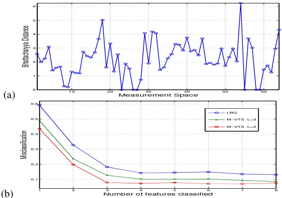
is shown as a 3D visualization in figure 10(c). Comparing figures 10(a) and (c), the location of the boundaries between ‘bone’ and ‘other tissue’ is fairly poor. This can be attributed to the difficulty differentiating the two chosen textures. However, the ‘muscle’ regions are fairly well defined. Despite these problems, the overall classification rate is 93%. The LBG classifier and M-VTS were used on the same OP measurement space and the classification errors were plotted for selecting most discriminant features (Figure 11) from the marginal Bhattacharyya space (shown in Figure 12(a)). The results confirm both that the sequential feature selection is effective and that M-VTS consistently outperforms a single resolution classifier. The choice of the level (i.e. L) at which to begin the top-down M-VTS will depend on the relative size of the structures in the data and the ratio of inter to intra class variance present. In the synthetic knee phantom the plot in figure 12(b) shows a marginal improvement by initializing M-VTS at level 4 rather than level 3 of the OP.
[image:12.612.148.471.363.474.2](a) (b) (c)
Fig. 10. Synthetic knee phantom image size128×128×128consisting of 4 texture types arranged approximately into background, bones, muscle and other. (a) 3D visualization of the original data. (b) Arrangement of principal regions in volume. (c) 3D visualization of labeled data.
(a) (b) (c) (d)
20 40 60 80 100 120 20
40 60 80 100 120
20 40 60 80 100 120
20
40
60
80
100
120
20 40 60 80 100 120 20
40 60 80 100 120
20 40 60 80 100 120 20
40
60
80
100
120
20 40 60 80 100 120 20
40 60 80 100 120
20 40 60 80 100 120
20
40
60
80
100
120
20 40 60 80 100 120 20
40
60
80
100
120
20 40 60 80 100 120 20
40 60 80 100 120
[image:12.612.109.513.539.695.2](a) 0 10 20 30 40 50 60 1
2 3 4 5 6
Measurement Space
Bhattacharyya Distance
(b) 1 2 3 4 5 6 7 8
0.1 0.2 0.3 0.4 0.5 0.6
Number of features classified
Misclassification
[image:13.612.162.450.66.269.2]LBG M−VTS L=3 M−VTS L=4
Fig. 12. (a) MarginalBI(i)of knee phantom features space from OP. (b) Classification error comparing LBG against M-VTS atL= 3
and L= 4for sequential selection of features based on the BS feature selection. M-VTS is has consistently lower misclassification errors (about half of LBG with 3 or more features).
C. 3D MRI texture segmentation
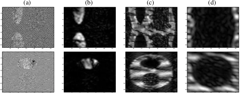
A set of experiments was conducted with 3D MRI sets of human knees acquired under different protocols: one set with Spin Echo and two sets with SPGR. In the three cases each slice had dimensions of 512×512 pixels and 87, 64 and 60 slices respectively. One sample slice from each set is presented in Figure 14(a). The bones, background, muscle and tissue classes were hand labeled to provide ground-truth for evaluation.
For the first data set, Case 1, the following classification approach was followed. Four training regions of size
32×32×32elements were manually selected for the classes ofbackground, muscle, boneandtissue. These training regions were small relative to the size of the data set, and they remained as part of the test data. Each training sample was filtered with the OP subband filtering scheme, and the results were used to construct the Bhattacharyya space (figure 13(a)).
It can be immediately noticed that two bands: S22,54, which correspond to the low pass bands, dominate the discrimination while the distance of the pairbone-tissueis practically zero compared with the rest of the space. If the marginals are calculated directly the low pass would dominate and the discrimination of the bone and tissue classes, which are difficult to segment, and could have easily been merged. Figure 13(b) zooms into the Bhattacharyya space of the bone-tissue pair. Here we can see that some features: S12,5,8,38,..., provide discrimination between bone and tissue, and the low pass bands help discriminate the rest of the classes.
Feature selection was performed with the Bhattacharyya space and 7 measurements were selected: S22 and
S12,5,8,39,9,51. This selection of features reduced significantly the computational burden. The final misclassification
obtained was 8.1% with 7 features. The result for 2D classification was 8.6% (figure 14(b)). For the M-VTS misclassification results were 6.0% (figure 14(c)). While the results from the 2D and 3D single resolution are close, the use of multiresolution improves the results by more than 2%. The classification with a multiresolution algorithm improves the results and produces a much smoother region classification. Some of the errors are due in part to magnetic inhomogeneity artifacts across the image that were not handled explicitly. It should be noted that the classification results, although not anatomically perfect, illustrate the utility of the use of texture features in MRI classification.
The SPGR MRI data sets were classified and the bone was segmented with the objective of using this as an initial condition for extracting the cartilage of the knee. The cartilage adheres to the condyles of the bones and appears as a bright, curvilinear structure in SPGR MRI data. Besides the low pass,S22, three high frequency bands were selected, namely S1,5,9.
(a)
Back−Musc Back−Bone
Back−Tiss Musc−Bone
Musc−Tiss Bone−Tiss
10 20 30 40 50 60 0
10 20 30 40 50 60
Feature Space
Bhattacharyya Distance
(b) 0 10 20 30 40 50 60
0.1 0.2 0.3 0.4 0.5 0.6 0.7 0.8 0.9 1
Feature Space
[image:14.612.155.453.101.299.2]Bhattacharyya Distance
Fig. 13. Knee MRI: (a) Bhattacharyya spaceB (3D, order 2), (b) Bhattacharyya space (Bi(bone, tissue)).
(a) (b) (c)
[image:14.612.146.471.373.701.2]bone mask. The knee was classified with LBG and M-VTS at level 3. One slice of the classified results is presented in the middle row of figure 14. As expected, M-VTS presents smoother results and reduces the misclassification of the bone from 32.8% to 10.5%. For Case 3 (bottom row of Figure 14) the reduction was from 57.8% to 24.2% with the unsupervised LBG method and if training data was used, the misclassification went down from 36.0% down to 12.0% with NN (table II).
Figure 15(a) presents a volume rendering of the segmented bone of Case 1. The four boney structures present in the MRI data set are clearly identifiable:patella, fibula, femur and tibia, and (b) shows a cloud of points of the bone class of Case 3. Here the misclassification is noticeable in the upper part of the patella (knee-cap), which is classified as background, and the lower part extends more than it should do into surrounding soft tissue (the infrapatellar pad).
[image:15.612.184.426.218.429.2](a) (b)
Fig. 15. (a) Rendering of the segmented bone of Case 1 (misclassification 8.1%) and (b) the segmented bone˜b(as clouds of points) from Case 3 (misclassification 12.0%).
D. Segmentation of the cartilage
Segmentation of articular knee cartilage is important to understand the progression of diseases such as ose-toarthritis and it enables the monitoring of therapy and effectiveness of new drug treatments [50], [51], [52]. MRI has played an important role since it is a 3D, non-invasive imaging method which is cheaper and less traumatic than arthroscopy, and has been the gold standard for cartilage assessment [53].
In this section, we propose a simple technique to extract the cartilage without the use of deformable models or seeding techniques. The user has to determine a Region of Interest (ROI) and a gray level threshold with the bone extracted from the previous section being used as a starting point. In order to segment the cartilage out of the MRI sets, two heuristics were used: cartilage appears bright in the SPGR MRIs, and cartilage resides in the region between bones. This is translated into two corresponding rules: threshold voxels above a certain gray level, and discard those not close to the region of contact between bones. The methodology to extract the cartilage followed these steps: extract the boundary of the bone segmented by the M-VTS; dilate this boundary by a number of elements to each side (5 voxels in our case); eliminate the elements outside the ROI and the dilated boundary; threshold the region (gray level g= 550for Case 2, and g= 280for Case 3); finally, eliminate isolated elements. It should be noted that the ROI is a cuboid and not an elaborate anatomical template.
(a) (b) (c)
Fig. 16. Cartilage of Case 2. (a) Slice 15 of the set with the cartilage in white. (b) Slice 46 of the set with the cartilage in white. (c) Rendering of the cartilage segmented from Case 2 and one slice of the MRI Set.
(a) (b) (c)
Fig. 17. Cartilage of Case 3. (a,b) The cartilage from two different view angles, (c) The Cartilage and one slice of the MRI Set.
VII. CONCLUSIONS
A multiresolution algorithm based on Fourier domain filtering was presented for the classification of texture volumes. Textural measurements were extracted in 3D data by subband filtering with an Orientation Pyramid tessellation. Some of the measurements can be selected to form a new feature space and their selection is based on their discrimination powers obtained from a novel Bhattacharyya space. A multiresolution algorithm was shown to improve the classification of these feature spaces: oct trees were formed with the features. Once the classification is performed at the a higher level of the tree, the class and boundary conditions of the elements are propagated down. A boundary refinement method with pyramidal, volumetric butterfly filters is performed to regain spatial resolution. This refinement technique outperforms a standard MRF approach. The algorithm presented was tested with artificial 3D images, a phantom type artificial textured volumes and MRI sets of human knees (both SPGR and T2 weighted sequences). Satisfactory classification results were obtained in 3D at a modest computational cost. In the case of the MRI data, M-VTS exploits well the textural characteristics of the data. The resulting seg-mentations of bone provide a good starting point for other techniques, such as deformable models, which are more sophisticated and require some initial conditions. If M-VTS is to be used for medical applications, extensive clinical validation is required and, in the case of MRI, the effects of inhomogeneities artifacts should be addressed. Furthermore, there is manual intervention in determining the number of classes, the size of the butterfly filters, the depth of the OP decomposition and the height of the OT used by the coarse-to-fine refinement. Further research might be focused in these areas.
VIII. ACKNOWLEDGEMENTS
This work was partly supported by CONACYT - M´exico. Dr Simon Warfield provided some of the MRI data sets and also kindly reviewed the results. Professor Roland Wilson and Dr Nasir Rajpoot are acknowledged for their valuable discussions on this work and help in revising the manuscript. The test data sets along with the software are available on an “as is” basis on the author’s web page: http://www.dcs.warwick.ac.uk/∼creyes/m-vts.
REFERENCES
[image:16.612.150.465.226.338.2][2] W. M. Wells, W. E. L. Grimson, R. Kikinis, and F.A. Jolesz. Adaptive segmentation of MRI data. IEEE Trans. on Medical Imaging, 15(4):429–442, 1996.
[3] M. Styner, C. Brechb¨uhler, G. Sz´ekely, and G. Gerig. Parametric estimate of intensity inhomogeneities applied to mri.IEEE Transactions
on Medical Imaging, 19(3):153–165, 2000.
[4] R. M. Haralick. Statistical and Structural Approaches to Texture. Proceedings of the IEEE, 67(5):786–804, 1979. [5] G. R. Cross and A. K. Jain. Markov Random Field Texture Models. IEEE Trans. on PAMI, PAMI-5(1):25–39, 1983.
[6] J. M. Keller and S. Chen. Texture Description and Segmentation through Fractal Geometry. Computer Vision, Graphics and Image
Processing, 45:150–166, 1989.
[7] M. Unser. Texture Classification and Segmentation Using Wavelet Frames. IEEE Trans. on Image Processing, 4(11):1549–1560, 1995. [8] S. Livens, P. Scheunders, G. Van de Wouwer, and D. Van Dyck. Wavelets for texture analysis, an overview. In6th Int. Conf. on Image
Processing and its Aplplications, volume 2, pages 581–585, Dublin, Ireland, july 1997.
[9] T. Randen and J. H. Husøy. Filtering for Texture Classification: A Comparative Study. IEEE Trans. on PAMI, 21(4):291–310, 1999. [10] M. Eden M. Unser. Multiresolution Feature Extraction and Selection for Texture Segmentation. IEEE Trans. on PAMI, 11(7):717–728,
1989.
[11] R. Wilson and M. Spann. Finite Prolate Spheroidal Sequences and Their Applications: Image Feature Description and Segmentation.
IEEE Trans. PAMI, 10(2):193–203, 1988.
[12] P. de Rivaz and N. G. Kingsbury. Complex Wavelet Features for Fast Texture Image Retrieval. InProc. ICIP 1999, pages 109–113, 1999.
[13] R. A. Lerski et.al. MR Image Texture Analysis - An Approach to Tissue Characterization. Mag. Res. Imaging, 11(6):873–887, 1993. [14] L. R. Schad, S. Bluml, and I. Zuna. MR Tissue Characterization of Intracrianal Tumors by means of Texture Analysis. Mag. Res.
Imaging, 11:889–896, 1993.
[15] COST European Cooperation in the field of Scientific and Technical Research. COST B11 Quantitation of MRI Texture. http://www.uib.no/costb11/, 2002.
[16] D. James et al. Texture Detection of Simulated Microcalcification Susceptibility Effects in MRI of the Breasts. J. Mag. Res. Imaging, 13:876–881, 2002.
[17] T. Kapur. Model based three dimensional Medical Image Segmentation. PhD thesis, AI Lab, Massachusetts Institute of Technology, May 1999.
[18] N. Saeed and B. K. Piri. Cerebellum Segmentation Employing Texture Properties and Knowledge based Image Processing : Applied to Normal Adult Controls and Patients. Magnetic Resonance Imaging, 20:425–429, 2002.
[19] I. J. Namer O. Yu, Y. Mauss and J. Chambron. Existence of contralateral abnormalities revealed by texture analysis in unilateral intractable hippocampal epilepsy. Magnetic Resonance Imaging, 19:1305–1310, 2001.
[20] Vassili A Kovalev, Frithjof Kruggel, and D. Yves von Cramon. Gender and age effects in structural brain asymmetry as measured by MRI texture analysis. NeuroImage, 19(3):895–905, 2003.
[21] J. M. Mathias, P. S. Tofts, and N. A. Losseff. Texture Analysis of Spinal Cord Pathology in Multiple Sclerosis. Mag. Res. in Medicine, 42:929–935, 1999.
[22] K. Fukunaga. Introduction to Statistical Patt Rec. Academic Press, 1972.
[23] N.M. Rajpoot. Texture Classification Using Discriminant Wavelet Packet Subbands. InProc. IEEE Midwest Symposium on Circuits
and Systems, Aug. 2002.
[24] A. Bhalerao and C.C. Reyes-Aldasoro. Volumetric Texture Description and Discriminant Feature Selection for MRI. In Proceedings
of Eurocast’03, Canarias, Spain, February 2003.
[25] P. Schroeter and J. Bigun. Hierarchical Image Segmentation by Multi-dimensional Clustering and Orientation-Adaptive Boundary Refinement. Patt Rec, 28(5):695–709, 1995.
[26] L. Blot and R. Zwiggelaar. Synthesis and Analysis of Solid Texture: Application in Medical Imaging. In Texture 2002: 2nd Int
Workshop on Texture Analysis and Synthesis, pages 9–14, Copenhagen, 1 June 2002.
[27] M. J. Chantler. Why Illuminant Direction is fundamental to Texture Analysis.IEE Proceedings in Vision, Image and Signal Processing, 142(4):199–206, 1995.
[28] K. J. Dana, B. van Ginneken, S. K. Nayar, and J. J. Koenderink. Reflectance and texture of real-world surfaces.ACM Trans. Graphics, 18(1):1–34, 1999.
[29] F. Neyret. A general and Multiscale Model for Volumetric Textures. In Graphics Interface, Qu´ebec, Canada, 17-19 May 1995. [30] B. K. Bay. Texture correlation. A method for the measurement of detailed strain distributions within trabecular bone. J of Orthopaedic
Res, 13(2):258–267, 1995.
[31] I. Guyon and A. Elisseeff. An Introduction to Variable and Feature Selection. J of Machine Learning Research, 3(7-8):1157–1182, 2003.
[32] M. Dong and R. Kothari. Feature subset selection using a new definition of classifiability. Patt Rec Letts, 24(9-10):1215–1225, 2003. [33] R. Kohavi and G. H. John. Wrappers for feature subset selection. Artificial Intelligence, 97(1-2):273–324, 1997.
[34] T. Kailath. The Divergence and Bhattacharyya Distance Measures in Signal Selection. IEEE Trans. Commun. Technol., 15(1):52–60, 1967.
[35] A. Bhalerao and N. Rajpoot. Selecting Discriminant Subbands for Texture Classification. InBMVC, Norwich, UK, September 2003. [36] G. B Coleman and H. C Andrews. Image Segmentation by Clustering. Proceedings of the IEEE, 67(5):773–785, 1979.
[37] Trygve Randen and John H˚akon Husøy. Filtering for Texture Classification: A Comparative Study.IEEE Trans. Pattern Anal. Machine
Intel., 21(4):291–310, 1999.
[38] J. Kittler. Feature Selection and Extraction. In Y. Fu, editor, Handbook of Pattern Recognition and Image Processing, pages 59–83, New York, 1986. Academic Press.
[40] T. Ojala, K. Valkealahti, E. Oja, and M. Pietik¨ainen. Texture discrimination with multidimensional distributions of signed gray level differences. Patt Rec, 34(3):727–739, 2001.
[41] N. Malpica, J. E. Ortu˜no, and A. Santos. A multichannel watershed-based algorithm for supervised texture segmentation. Patt Rec
Letts, 24(9):1545–1554, 2003.
[42] R. Wilson and C.-T. Li. A Class of Discrete Multiresolution Random Fields and its Application to Image Segmentation. IEEE Trans.
Pattern Anal. Machine Intel., 25(1):42–56, 2003.
[43] P. J. Burt and E. H. Adelson. The Laplacian Pyramid as a compact Image Code. IEEE Trans. Commun., 31(4):532–540, 1983. [44] V. Gaede and O. G¨unther. Multidimensional access methods. ACM Computing Surveys, 30(2):170–231, 1998.
[45] H. Samet. The Quadtree and Related Hierarchical Data Structures. Computing Surveys, 16(2):187–260, 1984.
[46] M. Spann and R. Wilson. A quad-tree approach to image segmentation which combines statistical and spatial information. Patt Rec, 18(3/4):257–269, 1985.
[47] Edward R. Dougherty and Marcel Brun. A probabilistic theory of clustering. Patt Rec, 37(5):917–925, 2004. [48] T. Kohonen. Self-Organizing Maps. Springer, Berlin, Heidelberg, New York, third extended edition, 2001.
[49] Y. Linde, A. Buzo, and R.M. Gray. An Algorithm for Vector Quantizer Design. IEEE Trans. Commun., 28(1):84–95, 1980.
[50] J. A. Lynch, S. Zaim, J. Zhao, A. Stork, C. G. Peterfy, and H. K. Genant. Cartilage segmentation of 3D MRI scans of the osteoarthritic knee combining user knowledge and active contours. InProceedings of SPIE, 2000.
[51] L. M. Lorigo, O. D. Faugeras, W. E. L. Grimson, R. Keriven, and R. Kikinis. Segmentation of Bone in Clinical Knee MRI Using Texture-Based Geodesic Active Contours. InMICCAI, pages 1195–1204, Cambridge, USA, October 11-13 1998.
[52] S. K. Warfield, M. Kaus, Ferenc A. Jolesz, and Ron Kikinis. Adaptive, Template Moderated, Spatially Varying Statistical Classification.
Medical Image Analysis, 4(1):43–55, Mar 2000.
[53] I. van Breuseghem. Ultrastructural MR imaging techniques of the knee articular cartilage: problems for routine clinical application.
![Fig. 4.(a) 16-class natural texture mosaic (image f from Randen [37]). (b) Classification result using BS selected features](https://thumb-us.123doks.com/thumbv2/123dok_us/9754849.476487/7.612.164.446.66.415/natural-texture-mosaic-randen-classication-result-selected-features.webp)