Master Thesis, July 2017
Author:
Suzanne A. Thomasson
Supervisors: University of Twente: Dr.ir. L.L.M. van der Wegen Dr. M.C. van der Heijden
ORTEC: Dr.ir. G.F. Post Rogier Emmen
University of Twente
In order to complete the master Industrial Engineering and Management, I have been working on my Thesis since February 2017. I had the privilege of doworking this project at ORTEC -Optimization Technology. There are a few people that I would like to thank for helping me through this important part of my study.
First of all I would like to thank my supervisors from ORTEC, Rogier Emmen and Ger-hard Post. Your positivity and trust in my capabilities encouraged me to go the extra mile and make me enthusiastic for the topic of forecasting. I want to specifically thank Rogier for taking all the time in the world to teach me all there was to know on forecasting at ORTEC, and your ‘Code academy’ made me realise that programming can be fun after all. Also I would like to thank all colleagues that made my time at ORTEC so much fun that I want to keep working there.
Also, I would like to thank my first supervisor Leo van der Wegen for the great guidance. You always made time to read my thesis and to give critical feedback, which I highly appre-ciate. Your insights helped me lift my thesis to a higher level. Also, I would like to thank Matthieu van der Heijden who became my second supervisor at one of the last stages of the project. You had to read my thesis on very short notice, but nevertheless, you gave feedback that helped me gain interesting new insights.
Furthermore, I want to thank my parents who always showed unconditional pride and support during the entire course of my study. During the last five years, you were the most important encouragement to pass and make you proud. Also, I want to thank my friends that made my student life unforgettable. Finally, I want to thank my boyfriend for his sup-port, encouragement and care during this sometimes stressful period. Moving to Den Haag together with you made the end of my life as a student a lot better.
Den Haag, July 2017
ORTEC has a customer, Company X, that distributes liquefied petroleum gas (LPG) to clients in the Benelux for which ORTEC should decidewhen to replenish and how much to deliver. This is part of the inventory routing product OIR. To be able to do this, ORTEC has a forecasting engine in which generally three methods are used to predict LPG demand: the degree days method (with the yearly script) that is based on the temperature dependency of LPG demand, simple exponential smoothing (SES) with period 1 day, and SES with period 7 days (for datasets that show a within week pattern). The forecast horizon that is required is one week. The time buckets used to predict are one day of length (irrespective of the frequency of observations, weekly or even more infrequent data is disaggregated to daily data). However, they did not know how well this methodology performs and if it is suitable for each client of Company X. We do know that in 38% of the trips, one or more customers did not get their delivery, because the truck was empty before having visited all customers on the planned route. A reason for this could be that the truck driver had to deliver more LPG than planned at the customers earlier on the route due to bad forecasts. Only in 11.5% of the deliveries, the customer received exactly the planned amount of LPG. In order to get insight into this matter, we stated the main research question:
Can, and if so, how can the forecast performance of LPG demand be improved?
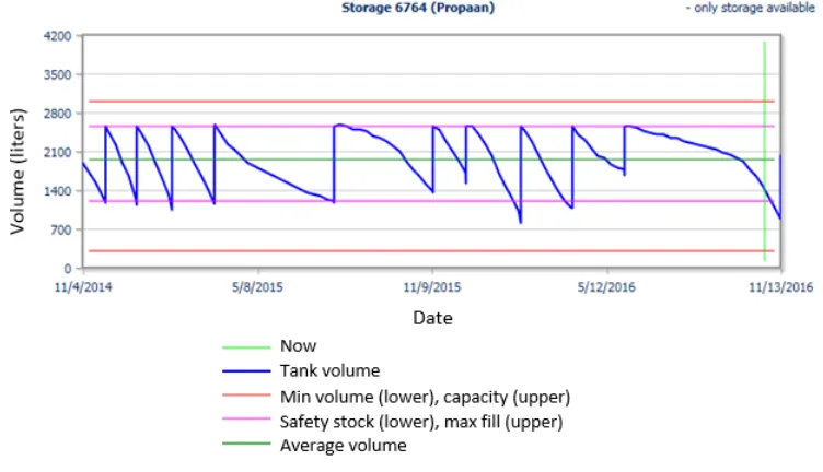
We categorised the clients of Company X into four categories: ‘Category 1’ for customers with only a few measurements (no telemetry system) and possibly yearly seasonality, ‘Cate-gory 2’ for clients that show a lot of ‘negative’ usage (the measuring equipment is inaccurate in the sense that it is not able to compensate for volume changes caused by fluctuations in temperature, which leads to the volume being above, and directly after, below a certain threshold resulting in supposedly negative usage), ‘Category 3’ for clients with weekly data and no seasonality, and ‘Category 4’ for customers with weekly data and yearly seasonality (sinus shaped). Figure 1 shows what representative datasets of these categories look like and the percentage indicates how many customers fall within each category.
(c) Category 3: weekly data, no seasonality (3%) (d) Category 4: weekly data, yearly seasonality (35%)
Figure 1: Categories of datasets
instead of discarding it. After classifying 2284 datasets on category, we found that 38% of them is ‘Category 2’ which means that the problem is of substantial size. The number of deliveries to ‘Category 2’ storages can be reduced by 87% when sending negative usage to the forecasting engine.
After solving the data issues, we investigated which forecasting method is most suitable per data category. We found that suitable methods for temperature dependent time series are: Holt-Winters (additive and multiplicative) and linear regression (simple and multiple, using climatological variables as external variables). For the series without seasonality, suit-able methods are: simple exponential smoothing (SES) and moving average. For the datasets that show intermittent demand patterns, that result from the inaccuracy of the measuring equipment, appropriate methods are: SES, Croston’s method, and the TSB method. Besides, there is proof for the accuracy and robustness of combining forecasts. An important finding is that the performance of the methods should not be expressed in terms of mean average percentage error (MAPE), because it is unreliable for low volume datasets. Instead, the root mean squared error (RMSE) should be used.
line is predicted with SES, and finally the temperature dependency is added again).
Besides forecasting, we investigated automating model selection. Currently, for each dataset, the user has to choose a forecast script manually. Time could be saved by automat-ing this. We looked at the possibilities of classification. After implementautomat-ing different methods, we conclude that logistic regression performs best in terms of accuracy, interpretability, and ease of implementation. This method is able to classify the data with an accuracy of 98.4% in WEKA.
Based on these findings, we recommend the following to improve the current forecasting procedure:
- Make the after delivery readings irrelevant in OIR for all storages, except for ‘Category 1’ datasets
- Forecast ‘Category 2’ datasets with simple exponential smoothing and the rest with the degree-days method
- Implement Cook’s distance before calculating the regression coefficients
- Send the measurements that show negative usage to the forecasting engine instead of discarding them
- Use the RMSE instead of the MAPE as performance indicator
- Implement simple linear regression for the degree-days method
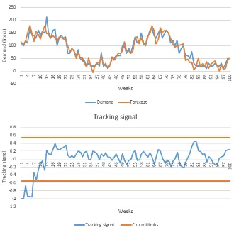
- Compute a tracking signal to monitor whether the forecasting system remains in control using an α of 0.1 and control limits of ±0.55, but only for ‘Category 3’ and ‘Category 4’ datasets
- Use logistic regression as classification method
Preface I
Management Summary III
1 Introduction 1
1.1 Background ORTEC and research motive . . . 1
1.2 Research goal and research questions . . . 2
2 Review of existing literature 5 2.1 Short term gas demand . . . 5
2.2 Moving average method . . . 6
2.2.1 Single moving average . . . 6
2.2.2 Double moving average . . . 7
2.3 Exponential smoothing . . . 7
2.3.1 Simple exponential smoothing . . . 9
2.3.2 Double exponential smoothing . . . 10
2.3.3 Holt’s linear trend method . . . 10
2.3.4 Additive damped trend method . . . 11
2.3.5 Holt-Winters method . . . 11
2.3.6 Holt-Winters damped method . . . 12
2.3.7 Parameter estimation and starting values . . . 13
2.3.8 Conclusion . . . 13
2.4 Intermittent demand . . . 13
2.4.1 Croston’s method . . . 14
2.4.2 SBA method . . . 14
2.4.3 TSB method . . . 14
2.5 Regression models . . . 16
2.5.1 Simple linear regression . . . 16
2.5.2 Multiple linear regression . . . 17
2.6 Degree days method . . . 21
2.7 Covariates . . . 24
2.8 Artificial Neural Networks (ANN) . . . 25
2.9 Combining forecast methods . . . 28
2.10 Forecast performance . . . 29
2.11 Sample size . . . 31
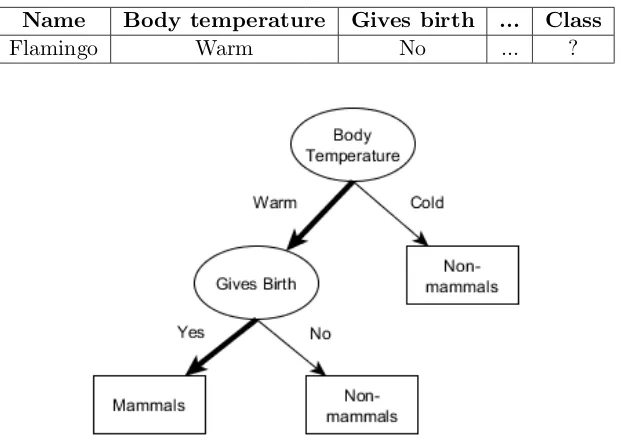
2.12 Classification . . . 32
2.12.1 Decision tree methods . . . 33
2.12.2 k-Nearest Neighbour (kNN) . . . 36
2.12.4 Artificial neural networks . . . 37
2.12.5 Classification performance . . . 37
2.13 Conclusion . . . 39
3 Current situation 41 3.1 Datasets of storages . . . 41
3.2 Current forecasting procedure . . . 44
3.2.1 Dependency on temperature . . . 44
3.2.2 Degree-days method . . . 46
3.2.3 Yearly script . . . 48
3.2.4 Issues . . . 50
3.3 Data patterns . . . 50
3.4 Conclusion . . . 53
4 Selecting forecasting methods 55 4.1 Data cleaning . . . 55
4.2 Parameter estimation . . . 58
4.3 Category 1 . . . 59
4.4 Category 2 . . . 60
4.5 Category 3 . . . 63
4.6 Category 4 . . . 65
4.6.1 Tracking signal . . . 68
4.7 Conclusion . . . 70
5 Automatic model selection: Classification 71 5.1 Attribute choice . . . 71
5.2 Classification methods . . . 72
5.3 Conclusion . . . 75
6 Conclusion and recommendations 77 6.1 Conclusion . . . 77
6.2 Recommendations . . . 78
6.3 Suggestions for further research . . . 78
Bibliography 81
Appendix 85
A Correlations external variables 87
B Statistical tests regression models 89
C Data cleaning: reading after 91
D Category 1 forecasting 93
E Category 2 forecasting 95
F Category 3 forecasting 97
Introduction
The world around us is becoming more and more dynamic. Companies are finding ways to become more efficient and predict the future in order to stay ahead of competition. ORTEC is a leading company in helping companies to achieve this. This report introduces the problem that ORTEC currently has to deal with. Section 1.1 gives some background on the company and introduces the research motive. Section 1.2 gives the goal of the research and states the research questions.
1.1
Background ORTEC and research motive
ORTEC is one of the world’s leaders in optimization software and analytic solutions. Their purpose is to optimize the world with their passion for mathematics. Currently, ORTEC has developed a tool that can forecast one time series using at most one external variable, for example sales and the temperature outside. Ice-creams sell better when it is hot outside, than temperature can be used to improve the forecast. However, more and more customers demand forecasting of more variables that influence each other. The topic of research is the situation where several aspects together generate the output to forecast.
Currently, ORTEC has a client, Company X, that distributes LPG to its clients. These clients have one or several LPG bulk tanks (which we call storages from now on). Generally, every one or two weeks, Company X receives inventory levels of the storages belonging to the clients. Since it is inefficient to replenish frequently, ORTEC forecasts the LPG usage in order to predict when to do this, namely, just before the client is out of stock. Also, forecasts are required to determine how much LPG should be delivered to each storage. Company X and its clients have what is called a Vendor Managed Inventory (VMI) system: a supply-chain initiative where the supplier is authorized to manage inventories of agreed-upon stock-keeping units at retail locations (C¸ etinkaya & Lee, 2000). By this, inventory and transportation deci-sions are synchronized. This relationship allows Company X to consolidate shipments which means that rides can be combined and less transportation is required. This project is part of the product ‘ORTEC Inventory Routing (OIR)’, and ORTEC is asked by Company X to determine when to replenish and how much.
visited and the number of customers visited on a route varies from 2 to 20. We do not know how often it occurs that LPG remains after having visited all customers on the route but we do know thatin 38% of the routes, one or more customer could not get its delivery, because the truck was already empty. Only in 11.5% of the deliveries, the truck driver delivers exactly the planned amount of LPG.
The fact that the inventory level is given every one or two weeks but the outside tem-perature is given on a daily basis and daily forecasts are needed, makes it challenging to forecast correctly. Currently this forecast is done by simple exponential smoothing and the degree days method. Degree days are a simplified form of historical weather data that are used to model the relationship between energy consumption and outside air temperature. The method uses heating degree days (HDD) which are days that heating was necessary due to the cold weather and cooling degree days (CDD) for when air-conditioning is used when it is hot outside. For example, when the outside air temperature was 3 degrees below the base temperature for 2 days, there would be a total 6 heating degree days. The same holds for CDD, but then the degree days are calculated by taking the number of days and num-ber of degrees that the outside temperature was above that base temperature. Originally, this method is used to determine the weather-normalized energy consumption. Weather-normalization adjusts the energy consumption to factor out the variations in outside air temperature. For example, when a company consumed less energy in one year compared to the year before, weather-normalization can determine whether this was because the winter was a bit warmer or because the company was successful in saving energy. Normalisation is not necessary when forecasting. With the help of historical data on the energy consumption and number of degree days, a regression analysis can be used to determine the expected en-ergy consumption given the number of degree days. The method is explained in more detail later in the report. The advantage of this method is that degree-day data is easy to get hold of and to work with. Besides, it can come in any time scale, so also the one or two weeks that ORTEC has to work with.
Even though this method is easy to work with, ORTEC does not know exactly how good this method performs and if all customers benefit from this method. Also, they want to know whether there are other methods available and if there are other external variables (besides the temperature that is currently used) that could improve the forecast.
1.2
Research goal and research questions
Since ORTEC does not know how well the current forecasting methodology works, and whether other external variables (covariates) could improve the forecast, the main research question is:
Can, and if so, how can the forecast performance of LPG demand be improved?
In order to reach the research objective, several sub questions are answered:
1. What is known in literature on forecasting LPG demand or similar cases? (Chapter 2)
(a) Which methods are used in literature for forecasting LPG demand or similar cases? (b) How can forecast performance be measured?
Since the current situation requires quite some background information, the first question elaborates on this in Chapter 2. Scientific articles and books on forecasting are used.
2. What is the current situation at ORTEC? (Chapter 3)
(a) What method is currently used by ORTEC for forecasting LPG demand of the smaller clients of Company X?
(b) What are the issues of this methodology? (c) What are the characteristics of the data?
This second question is answered in Chapter 3. For this question and its sub questions, interviews with the persons currently working on the project have to be performed, which are persons working on the forecast software but also persons that have been working on the business case and have been in contact with Company X. Question 2b is answered by finding out what patterns are present in the data and on which relationship(s) the current methodology is based and investigating how suitable this is. The third sub question is answered by analysing datasets of different customer types.
3. Which methods are eligible for ORTEC? (Chapter 4)
(a) How should the data be cleaned to be suitable for forecasting? (b) How can the current methodology be improved?
(c) Which method performs best and is most suitable?
To answer these questions, we have to find out which inconsistencies and issues in the data should be corrected. After that, we try to improve the current methodology by making adjustments. Then statistical tools as R, SPSS, and simple visual plots are used in order to find trend and/or seasonality and other data patterns that help determine which other forecasting methods might be suitable for the data. Chapter 4 elaborates on this research question. Which method performs best is selected by using different performance indicators as the MSE, MAPE, and MAD, which are explained later.
4. How can classification methods be used for automatic method selection? (Chapter 5)
(a) How should the classification methods proposed in literature be used? (b) Which classifier performs best?
Review of existing literature
In order to answer the first research question ‘What is known in literature on forecasting LPG demand or similar cases?’, this chapter discusses what is available in literature on these topics to get some more insight. The sub questions answered are ‘Which methods are used in literature for forecasting LPG demand or similar cases?’ and ‘How can forecast performance be measured?’.
The first section briefly discusses short-term gas demand and which methods are broadly used in literature to forecast this. There are two common models that are based on projecting forward from past behaviour: moving average forecasting and exponential smoothing. The second section explains moving average and the third explains exponential smoothing and gives several alternative exponential smoothing methods that could be useful for predicting LPG demand. Moving average and exponential smoothing are time series models, which means that the dependent variable is only determined by time and/or previous values of the variable. However, causal models could also be useful for forecasting. In a causal model, external factors (other time series) form the explanatory variables of the dependent variable. For example, in the LPG case, the LPG demand could possibly also be dependent on the outside temperature which is an external factor (also called covariate).
Some of the best-known causal models are regression models, those are discussed in Section 2.5. Currently, ORTEC uses a causal model called the degree-days method. This method is explained in Section 2.6. Besides, there are models that combine time series and causal models. Those are discussed in Section 2.7. Since literature indicates that Artificial Neu-ral Networks (ANNs) could be helpful forecasting LPG demand, Section 2.8 explains this. Section 2.9 explains how combining different forecasting methods could improve forecast per-formance. In order to determine which of these methods performs best, it is necessary to find out how to measure forecast performance. This is explained in Section 2.10. Section 2.11 elaborates on the sample size required by each method. Section 2.12 addresses automatic model selection by classification. The chapter ends with a conclusion in Section 2.13.
2.1
Short term gas demand
elabo-rate on forecasting electricity demand in this chapter. Literature introduces and tests many electricity demand forecasting methods. This section gives a short introduction on what has been done in literature on this specific topic.
The aim of business forecast is to combine statistical analyses and domain knowledge to develop acceptable forecasts that will ultimately drive downstream planning activities and support decision making (Hoshmand, 2009). In production and inventory control, forecast-ing is a major determinant of inventory costs, service levels, and many other measures of operational performance (Gardner, 2006). It is used as a tool to make economic and busi-ness decisions on tactical, strategic, or operational level. Short-term load (electricity or LPG demand) forecasting is essential in making decisions on all those levels. Many operational decisions are based on load forecasts, under which the decision on when to replenish the LPG storages of several clients which should happen as less often as possible in order to save costs but the client may never run out of stock (Fan & Hyndman, 2010) but also how much to deliver to the customers. In order to do this, with the help of load forecasting, we need to predict when the clients are expected to be out of stock and how much LPG should be delivered.
Various techniques have been developed for electricity demand forecasting. Statistical models as linear regression-, stochastic process- and ARIMA models are widely adopted (Fan & Hyndman, 2010). Recently, machine learning techniques and fuzzy logic approaches have also been used and achieved relatively good performance (Fan & Hyndman, 2010). Exponen-tial smoothing has received more attention since the study of Taylor (2003). Since exponenExponen-tial smoothing is considered an easy in use method that gives relatively accurate results, OR-TEC uses this in combination with the degree-days method in order to forecast LPG demand.
Even though mostly electricity, but also natural gas demand, load forecasts are based on outside temperature, there are other exogenous variables that influence demand as work-ing days, weekends, feasts, festivals, cloud cover, and humidity (Kumru & Kumru, 2015). However, the main parameter that heavily influences demand is temperature.
2.2
Moving average method
The moving average approach takes the previousnperiods’ actual demand figures, calculates the average over these n periods, and uses this average as a forecast for the next period’s demand. The data older than the nperiods play no part in the next period’s forecast andn
can be set at any level (Slack et al., 2010). The advantage of this method is that it is very fast and easy to implement and execute. The main assumption in moving average models is that an average of past observations can be used to smooth the fluctuations in the data in the short-run (Hoshmand, 2009). As each observation becomes available, a new mean is computed by leaving out the oldest data point and including the newest observation.
2.2.1 Single moving average
The next equation shows how a moving average is computed:
Ft=
Yt−1+Yt−2+...+Yt−n
n (2.1)
where
Yt is the actual value at time periodt
nis the number of terms in the moving average
The choice ofnhas implications for the forecast. The smaller the number of observations, the forecast is only based on the recent past. The larger the number, the forecast is the average of the recent past and the further past. The first is desirable if the analyst encounters sudden shifts in the level of the series and a large number desirable when there are wide and infrequent fluctuations in the series (Hoshmand, 2009). Moving average is not able to cope with cyclical patterns as seasonality.
2.2.2 Double moving average
The single moving average method as just described is not able to cope with trend, seasonality, or cyclical patterns that could be present in the data. Double moving average is used when the time series data have a linear trend. The first set of moving averages (M At) is computed
as discussed in Subsection 2.2.1, and the second set is computed as a moving average of the first set (M A0t).
M At=Ft=
Yt−1+Yt−2+...+Yt−n
n (2.2)
M A0t= M At−1+M At−2+...+M At−n
n (2.3)
The difference betweenM Atand M A0t is computed as follows:
at= 2M At−M A0t (2.4)
Then the slope (trend) is measured by:
Tt=
2
n−1(M At−M A
0
t) (2.5)
With these, the forecast forx periods into the future can be made by:
Ft+x =at+Ttx (2.6)
where
Ft+x is the forecast valuex periods ahead
nis the number of periods in the moving average
Yt is the actual value at periodt
2.3
Exponential smoothing
Exponential smoothing forecasts demand in the next period by taking into account the actual demand in the current period and the forecast that was previously made for the current period, the details are explained later. The method relies on the assumption that the mean is not fixed over all time, but rather changes over time (Hoshmand, 2009). This chapter gives several methods of exponential smoothing. Before explaining the basics of these methods, the different methods are being classified using the method proposed by Pegels (1969) and later extended by Gardner (1985) and again by Taylor (2003). Table 2.1 gives an overview.
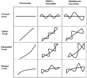
In a time series, trend could be present. Trend is defined as ‘long-term change in the mean level per unit time’. It can be additive (of constant size from year to year), or multiplicative (proportional to the local mean), or mixed (Chatfield, 2006) (see Figure 2.1). Another aspect that could be present in the time series is seasonality which could also be additive, multiplicative, or mixed. Table 2.1 gives the possible combinations.
[image:18.595.144.436.260.522.2]Figure 2.1: Additive and Multiplicative Seasonality (Gardner, 1985)
Table 2.1: Classification exponential smoothing (Hyndman, 2008)
De Gooijer & Hyndman (2006), of the methods described by Hyndman & Athanasopoulos (2014):
(N, N) = Simple exponential smoothing (Subsection 2.3.1) (A, N) = Holt’s linear method (Subsection 2.3.3)
(M, N) = Exponential trend method
(Ad, N) = Additive damped trend method (Subsection 2.3.4)
(Md, N) = Multiplicative damped trend method
(A, A) = Additive Holt-Winters method (Subsection 2.3.5) (A, M) = Multiplicative Holt-Winters method Subsection 2.3.5) (Ad, M) = Holt-Winters damped method (Subsection 2.3.6)
Since ORTEC mentioned that currently simple exponential smoothing is used, that is discussed in the next section. However, in literature, the Holt-Winters method is proposed as well performing exponential smoothing in the specific electricity demand case (Taylor, 2003; Taylor, 2010). Therefore that method is also discussed (Subsection 2.3.5). Since the trend methods assume a constant trend, forecasts using those often tend to over-forecast, especially for long-term forecasts. Therefore, also the damped trend methods are discussed.
One of the biggest advantages of exponential smoothing is the surprising accuracy that can be obtained with minimal effort in model identification (Gardner, 1985). There is substantial evidence that exponential smoothing models are robust, not only to different types of data but to specification error (Gardner, 2006). Many studies have found that exponential smoothing was at least as accurate as Box-Jenkins (ARIMA). However, a disadvantage of exponential smoothing in general is its lack of an objective procedure for model identification (Gardner & McKenzie, 1988). Besides, their usual formulations do not allow for the use of explanatory variables, also called predictors (Berm´udez, 2013).
2.3.1 Simple exponential smoothing
Simple exponential smoothing is a common approach based on projecting forward from past behaviour without taking into account trend and seasonality. It takes into account the actual demand of the current period and the forecast which was previously made for the current period, in order to forecast the value in the next period. It is also possible to forecast more periods into the future (x instead of 1), but this is not desirable since only the presence of a small trend already disrupts the forecast. The most recent observations play a more important role in making a forecast than those observed in the distant past (Hoshmand, 2009). The easiest form of exponential smoothing is:
Ft=αYt−1+ (1−α)Ft−1 (2.7) where
α is the smoothing constant
Yt−1 is the actual value of last period
Ft−1 is the forecasted value for last period
the distant past less important than the more recent ones like mentioned before (Hyndman, Koehler, Ord & Snyder, 2008).
This smoothing constantαmust be chosen when using the exponential smoothing method. In this easiest form of exponential smoothing, there is only one smoothing parameter, but later in this report methods containing several smoothing parameters are discussed. This parameters could be chosen based on experience of the forecaster but a more robust method is to estimate them from previous data. A way to do this is by using the sum squared error (SSE). These errors are calculated by:
n X
t=1
(Yt−Ft)2 (2.8)
whereYtis the actual value andFtis the forecasted value andnis the number of observations.
By minimizing the SSE, the values of the parameter(s) can be estimated (Price & Sharp, 1986). Section 2.10 gives other performance measurements on which the smoothing parameter can be estimated.
2.3.2 Double exponential smoothing
The simple exponential smoothing method is not able to handle trended data. Double ex-ponential smoothing methods on the other hand, are. Let us first discuss Brown’s double exponential smoothing, also known as Brown’s linear exponential smoothing (LES) that is used to forecast time series containing a linear trend (Hoshmand, 2009). The forecast is done by:
Ft+x=at+xTt (2.9)
where
Ft+x is the forecast value x periods into the future
Tt is an adjustment factor similar to a slope in a time series (trend)
x is the number of periods ahead to be forecast
To compute the difference between the simple and the double smoothed values as a measure of trend, we use the following equations:
A0t=αFt+ (1−α)A0t−1 (2.10)
A00t =αA0t+ (1−α)A00t−1 (2.11) whereA0t is the simple smoothed value andA00t is the double smoothed value. This leads to:
at= 2A0t−A 00
t (2.12)
Besides, the adjustment factor is calculated by:
Tt=
α
(1−α)(A
0
t−A00t) (2.13)
2.3.3 Holt’s linear trend method
little more flexibility. The shortcoming, however, is that determining the best combination between the two smoothing constants is costly and time consuming (Hoshmand, 2009). The following formula gives the forecast:
Ft+x =At+xTt (2.14)
with
At=αYt+ (1−α)(At−1+Tt−1) (2.15)
Tt=β(At−At−1) + (1−β)Tt−1 (2.16) where
At is the smoothed value
α is the smoothing constant (between 0 and 1)
β is the smoothing constant for the trend estimate (between 0 and 1)
Tt is the trend estimate
xis the number of periods to be forecast into the future
Ft+x is the forecast forx periods into the future
2.3.4 Additive damped trend method
As discussed before, Holt’s linear trend model, assumes a constant trend indefinitely into the future. In order to make forecasts more conservative for longer forecast horizons, Gardner & McKenzie (1985) suggest that the trends should be damped (Hyndman, 2014). This model makes the forecast trended on the short run and constant on the long run. The forecasting equation is as follows:
Ft+x=At+ (φ+φ2+...+φx)Tt (2.17)
with
At=αYt+ (1−α)(At−1+φTt−1) (2.18)
Tt=β(At−At−1) + (1−β)φTt−1 (2.19) whereφis the damping parameter (0< φ <1).
2.3.5 Holt-Winters method
The linear trend method can be adjusted when a time series with not only trend but also seasonality must be forecasted. The resulting method is known as the famous Holt-Winters method. The trend formula remains the same, only the formula forAt (level) and for Ft+x
change and an equation for seasonality is added (Taylor, 2003).
Additive Holt-Winters method
There are two types of seasonal models: additive (assumes the seasonal effects are of constant size) and multiplicative (assumes the seasonal effects are proportional in size to the local deseasonalised mean). Forecasts can be produced for any number of steps ahead (Chatfield, 1978). The forecast formula for the additive variant is adjusted to the following:
Ft+x=At+xTt+It−s+x (2.20)
TheAt formula becomes
and the following formula for seasonality is added
It=δ(Yt−At−1−Tt−1) + (1−δ)It−s (2.22)
where
δ is the smoothing constant for seasonality
It is the locals-period seasonal index Multiplicative Holt-Winters method
The forecast equation for the multiplicative variant is as follows:
Ft+x= (At+xTt)It−s+x (2.23)
and the formula for level At is
At=α
Yt
It−s !
+ (1−α)(At−1+Tt−1) (2.24)
and the seasonality formula is adjusted to
It=δ
Yt
At−1+Tt−1
!
+ (1−δ)It−s (2.25)
The Holt-Winters method is widely used for short-term electricity demand forecasting because of several advantages. It only requires the quantity-demanded variable, it is relatively simple, and robust (Garc´ıa-D´ıaz & Trull, 2016). Besides, it has the advantage of being able to adapt to changes in trends and seasonal patterns in usage when they occur. It achieves this by updating its estimates of these patterns as soon as each new observation arrives (Goodwin, 2010).
A disadvantage of the Holt-Winters method (both additive and multiplicative) is that it is not so suitable for long seasonal periods such as 52 for weekly data or 365 for daily data. For weekly data, 52 parameters must be estimated, one for each week, which results in the model having far too many degrees of freedom (Hyndman & Athanasopoulos, 2014). Ord & Fildes (2013) propose a method to make these seasonality estimates more reliable for the multiplicative variant. Instead of calculating the seasonals on individual series level, they calculate the seasonality of an aggregate series. This results in having less randomness in the estimates. For this, series with the same seasonality should be aggregated. For example, in the LPG case, more LPG is used in the winter and less in the summer so we expect that many clients follow the same usage pattern. When similar series are aggregated, individual variation decreases. This does not solve the problem of having to estimate many parameters but makes the estimation slightly more robust.
2.3.6 Holt-Winters damped method
As for Holt’s linear model, a damped version exists for the Holt-Winters method. The forecasting equation is:
Ft+x=At+ (φ+φ2+...+φx)Tt+It−s+x (2.26)
with the same equation for trend as the additive damped trend method:
Tt=β(At−At−1) + (1−β)φTt−1 (2.28) but adds an equation for seasonality:
It=δ(Yt−At−1−φTt−1) + (1−δ)It−s (2.29)
Also here, the damping factor is 0< φ <1.
2.3.7 Parameter estimation and starting values
In order to implement either of these exponential smoothing methods methods, the user must
- provide starting values for At,Tt, and It
- provide values forα,β, and δ
- decide whether to normalise the seasonal factors (i.e. sum to zero in the additive case or average to one in the multiplicative case) (Chatfield & Yar, 2010)
The starting- and smoothing values can be estimated in several ways that we describe in Chapter 4.
2.3.8 Conclusion
Concluding, there are many versions of exponential smoothing that are able to cope with either trend, seasonality, or both. The method that is used most in literature for forecasting electricity demand is the Holt-Winters method or a variant of this method. It is used because it is a relatively simple method in terms of model identification that gives surprisingly accurate results. On the other hand, when implemented for series with a long seasonal period (e.g. yearly seasonality with daily or weekly data), many parameters must be estimated which makes the model unstable. Important is, however, to determine which method suits the data best in terms of trend and seasonality. Both patterns could be additive, multiplicative, or neither of those. It is important to try different methods in order to find which is most suitable for the specific dataset.
2.4
Intermittent demand
2.4.1 Croston’s method
A widely used method is Croston’s method that differentiate between these two elements by updating demand size (st) and interval (it) separately after each period with positive demand
using exponential smoothing (Teunter et al., 2011). The notation is as follows (Pennings, Van Dalen, & Van der Laan, 2017):
ˆ
st+1|t= (
ˆ
st|t−1 ifst= 0
ˆ
st|t−1+α(st−sˆt|t−1) ifst>0
ˆi
t+1|t= (
ˆit|t−1 ifst= 0 ˆit|t−1+β(it−ˆit|t−1) ifst>0
and demand forecasts follow from the combination of the previous two forecasts:
ˆ
dt+1|t=
ˆ
st+1|t
ˆit+1|t (2.30)
where ˆ
dt+1|t is the demand forecast for next period (t+ 1)
ˆ
st+1|t is the demand size forecast for next period
ˆit+1|t is the interval forecast for next period
α and β are the smoothing constants, 0≤α, β≤1
2.4.2 SBA method
However, Syntetos & Boylan (2001) pointed out that Croston’s method is biased sinceE(dt) =
E(st/it)6=E(st)/E(it). A well supported adjustment is the SBA method which incorporates
the bias approximation to overcome this problem. Equation 2.30 is adjusted to:
ˆ
dt+1|t= 1−
β
2
!
ˆ
st+1|t
ˆit+1|t (2.31) whereβ is the smoothing constant used for updating the intervals.
However, as Teunter et al. (2011) point out, some bias remains with this adjustment, indeed there are cases where the SBA method is more biased than the original Croston method. Besides, the factor (1−β/2) makes the method less intuitive which may hinder implementation. Another disadvantage of both the Croston method as SBA is that the forecast is only updated after demand has taken place. When no demand occurs for a very long period of time, the forecast remains the same which might not be realistic (Teunter et al., 2011).
2.4.3 TSB method
Teunter et al. (2011) proposes not to update the inter-arrival time but the probability that demand occurs (ˆp). Therefore, the equations change to:
ˆ
st+1|t= (
ˆ
st|t−1 ifst= 0
ˆ
ˆ
pt+1|t= (
(1−β)ˆpt|t−1 ifst= 0
(1−β)ˆpt|t−1+β ifst>0
and the forecast becomes:
ˆ
dt+1|t= ˆpt+1|tsˆt+1|t (2.32)
which is the probability that demand occurs multiplied by the predicted demand size. This method reduces the probability that demand occurs each period with zero demand and this probability increases after non-zero demand occurs. The estimate of the probability of oc-currence is updated each period and the estimate of the demand size is updated only at the end of a period with positive demand.
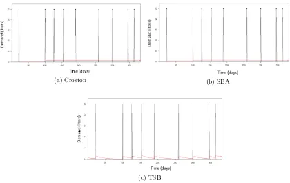
(a) Croston (b) SBA
[image:25.595.93.513.243.508.2](c) TSB
Figure 2.2: Forecasting intermittent demand
Figures 2.2a, 2.2b, and 2.2c show the differences between these methods. The red line represents the forecast. The data used for these figures is from Figure 3.13b but the unjust positive usages are compensated by the negative usages instead of excluding all negative us-ages. As expected, the forecast provided by SBA (0.533 liter/day) is slightly lower compared to Croston’s method (0.676 liter/day). The forecast given by TSB is higher than both (0.972 liter/day) since not so long ago, positive demand occurred.
periods and then 25 liters at once but is continuous over time. However, the measurement equipment is not able to measure continuous demand but only measures certain threshold values, for example each percent of the tank. Using these three methods on LPG data must prove which of the three performs best in another situation than the inventory control of spare parts.
2.5
Regression models
In Section 2.2 up and until 2.4, time series methods are discussed. As explained in the introduction, also causal models exist. Causal models assume that the variable to be fore-casted (called dependent or response variable) is somehow related to other variables (called predictors or explanatory variables). These relationships take the form of a mathematical model, which can be used to forecast future values of the variable of interest. As mentioned earlier, regression models are one of the best-known causal models (Reid & Sanders, 2005). This section explains two forms: simple linear regression (where one predictor influences the dependent variable) and multiple linear regression (where multiple predictors affect the dependent variable).
2.5.1 Simple linear regression
In the case of simple linear regression, where one predictor or explanatory variable predicts the value of the dependent variable, we are interested in the relationship between these two (X and Y). For example, a shopkeeper might be interested in the effect that the area of the shop (predictor, X) has on sales (dependent, Y) or an employer in the effect that age (predictor, X) has on absenteeism (dependent, Y). This is called a bivariate relationship (Hoshmand, 2009). The simplest model of the relationship between variable X and Y is a straight line, a so called linear relationship. This can both be used to determine if there is a relationship between both variables but also to forecast the value of Y for a given value of X. Such a linear relation can be written as follows:
Y =a+bX+ε (2.33)
where
Y is the dependent variable
X is the predictor (independent variable)
ais the regression constant, which is the Y intercept
b is the regression coefficient, in other words the slope of the regression line
εis the error term (a random variable with mean zero and a standard deviation of σ) The biggest advantage of this method is its simplicity. However, it is only successful if there is a clear linear relationship betweenX andY. An indicator for this linear relationship is thecoefficient of determination (R2) which is the fraction of the explained sum of squares of the total sum of squares. This is a statistical measure on how well the regression line approximates the real data.
The simple regression model cannot always be used. The model is based on some as-sumptions that must be met before being able to use regression:
- Normality
- Homoscedasticity
- Independence of errors
Normality requires the errors to be normally distributed. As discussed before, linearity can be checked by the coefficient of determinationR2 which is the squared correlation coefficient. Homoscedasticity requires the error variance to be constant. This means that when residuals are plot in a scatter plot, no clear pattern should be visible. Independence means that each error εt should be independent for each value of X (i.e. the residuals may not have
autocorrelation). The Durbin-Watson test checks for this auto-correlation of the residuals.
2.5.2 Multiple linear regression
Many dependent variables do not merely depend on one predictor. In this case, multiple regression can be used for forecasting purposes where one dependent variable is predicted by various explanatory variables. In this way, compared to simple regression, it allows to include more information in the model (Hoshmand, 2009). The regression coefficient is quite similar to that of simple regression:
Y =a+b1X1+b2X2+...+bnXn+ε (2.34)
where
Y is the dependent variable
X1...Xn are the predictors (independent variables)
a, b1, ..., bn are the partial regression coefficients
εis the error term (a random variable with mean zero and a standard deviation ofσ) The regression coefficients a,b1, b2,...,bk must be calculated while minimizing the errors
between the observations and predictions. This can be done with what is called the normal equation. Let y be the vector of observations, in the case of Company X this is a vector of actual usage. When m observations are available, y is a m-dimensional vector. X is a matrix that contains the values of the explanatory variables. The first column of this matrix contains only ones and the othern columns contain the values of the covariates where n is the number of predictors. X is a m×(n+ 1) matrix. The vector of regression coefficients (β), containing the constantaand coefficients b1,...,bn, is calculated as follows:
β = (XTX)−1XTy (2.35) This equation is not suitable forn greater than 10,000 since inverting a matrix that large is computationally intensive. Since we do not come close to using this much external variables, this method is suitable for this case.
The R2 is interpreted similarly as with simple regression but now gives the amount of variation that is explained by several explanatory variables instead of one.
For simple regression, several assumptions were mentioned. Violations of those assump-tions may present difficulties when using a regression model for forecasting purposes (Hosh-mand, 2009). Since we now have to deal with more than one predictor, an extra assumption is added: no multicollinearity which indicates that the different independent variables are not highly correlated.
- Linear dependency between independent variables and dependent variable
- Homoscedasticity
- Independence of errors (no auto-correlation)
- No multicollinearity
We now explain these assumption by using an example. The data that is used for this is an aggregate series of 21 temperature dependent time series that therefore show yearly seasonality. We choose to do this on an aggregate series in order to reduce variability of individual series.
Normality residuals
First it is important to determine whether the residuals are normally distributed. Figure 2.3 shows the P-P plot of the standardized residuals of the regression. When the expected cumulative probability is equal to the observed cumulative probability, normality can be assumed. This seems to be the case here.
According to the Shapiro-Wilk test, we can assume normality since the test statistic (0.991) is close to 1 which indicates that there is high correlation between the dependent variable demand and ideal normal scores. The test is explained in Appendix B.
Figure 2.3: Normality of independent variables
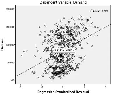
Linear dependency between independent variables and dependent variable
Secondly it must be checked whether there is a linear relationship between the independent variables and the dependent variable. This can be checked by making scatter plots. The scatter plots in Figure 2.4 show that the clearest linear relationship is between HDD and demand. Also global radiation shows a linear relation with demand. LPG price, relative humidity, and wind speed show a weak linear relationship with demand.
Homoscedasticity
Figure 2.4: Linear relationship between independent variables and dependent variable
LPG demand. When the error terms would have been heteroscedastic, meaning the residuals having different variances, theF-test and other measures that are based on the sum of squares of errors may be invalid (Hoshmand, 2009).
Figure 2.5: Homoscedasticity
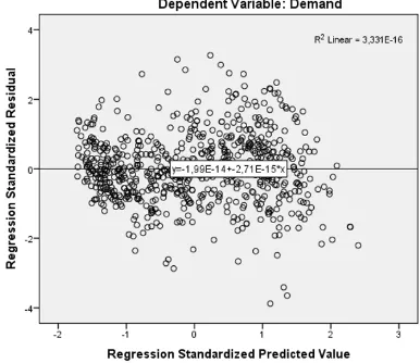
Independence of errors
[image:29.595.209.403.427.588.2]Figure 2.6 shows a plot of the residuals. It shows that these are independent. In other words, if the residuals are centred around zero throughout the range of predicted values, they should be unpredictable such that none of the predictive information is in the error. When the latter would have been the case, the chosen predictors are missing some of the predictive information. In our example, k = 5 and n = 700. The rule of thumb is that the
Figure 2.6: Independence of residuals
null hypothesis (the residuals are not autocorrelated) is accepted when 1.5< d <2.5, which is the case here since our d-value is 1.622. However, the critical value table for our k and
n values, givesdL = 1.864 anddU = 1.887 which would indicate that our null hypothesis is
rejected. It is therefore doubtful whether serious autocorrelation exists in this case.
No multicollinearity
The multicollinearity assumption states that predictor variables may not be highly correlated, in other words, they are independent of each other. It is wise to include the collinearity statistics in SPSS. Severe multicollinearity can result in the coefficient estimates to be very unstable. Multicollinearity implies that the regression model is unable to filter out the effect of each individual explanatory variable on the dependent variable (Hoshmand, 2009). An indicator for this problem is when there is a highR2but one or more statistically insignificant estimates of the regression coefficients (a and b1, ..., bk) are present. This can be solved by
simply removing one of the highly correlated variables. Four criteria must be checked:
- Bivariate correlations may not be too high
- Tolerance must be smaller than 0.01 (T olerance= 1−Rj2 whereR2j is the coefficient of determination of predictor j on all the other independent variables)
- Variance Inflation Factor (VIF) must be smaller than 10 (V IF = 1/tolerance), this would indicate that the variance of a certain estimated coefficient of a predictor is inflated by factor 10 (or higher), because it is highly correlated with at least one of the other predictors in the model
When all five independent variables (wind speed, HDD, humidity, global radiation, and LPG price) are forced into the model, the fourth criterion is violated. After removing relative humidity and LPG price from the model, multicollinearity is no problem. Removing those predictors does not jeopardize the R2 too much, namely from 86.9% to 86.7% which was expected since Hoshmand (2009) mentions that when one or two highly correlated predictors are dropped, theR2 value will not change much.
A big advantage of regression models is that they can deal with virtually all data patterns (Hoshmand, 2009). Also, it is a relatively easy model when the forecaster wishes to include one or more external variables. The disadvantage is that, as the name indicates, linear re-gression is only able to cope with linear relationships whereas relationships between variables could be of non-linear nature as well.
2.6
Degree days method
It is broadly agreed upon that the outside air temperature has a large effect on the electricity demand (Kumru & Kumru, 2015; Berm´udez, 2013; Garc´ıa-D´ıaz & Trull, 2016; Bessec & Fouquau, 2008). Currently, ORTEC uses the degree days method (among others) to include temperature in the LPG forecast. This section explains this method and gives its advantages and shortcomings.
Heating- and Cooling degree days
This method makes a distinction between heating degree days (HDDs) and cooling degree days (CDDs). HDDs come with a base temperature (that should be found by optimising theR2 when correlating demand with the corresponding HDDs, varying the base tempera-ture) and provide a measure of how many degrees and for how long the outside temperature was below that base temperature (using the average of the minimum- and maximum tem-perature of a specific day). For example, when the outside air temtem-perature was 3 degrees below the base temperature for 2 days, there would be a total of heating degree days of 6. The advantage of using HDDs over temperature in forecasting is that these HDDs can be aggregated over the time buckets that the user wants to forecast on. CDDs are calculated in a similar fashion, but then the degree days are calculated by taking the number of days and number of degrees that the outside temperature was above that base temperature. This base temperature could be another base temperature than that of HDDs. Moral-Carcedo & Vic´ens-Otero (2005) state that it is not trivial whether to use one or two thresholds. Hav-ing one threshold indicates that when the threshold temperature is passed, there is a sharp change in behaviour whereas when having two thresholds, it is assumed that in between these two thresholds, there is no appreciable change in demand. In other words, there is a neutral zone for mild temperatures where demand is inelastic to the temperature (Bessec & Fouquau, 2008; Psiloglou, Giannakopoulos, Majithia, & Petrakis, 2009).
In formula form the number of degree days is calculated by:
HDDs=Pnd
j=1max(0;T∗−tj) andCDDs=Pndj=1max(0;tj−T∗) where ndis the number
of days in the period over which the user wants to calculate the number of HDDs,T∗ is the threshold temperature of cold or heat, and tj the observed temperature on day j
Base temperature(s)
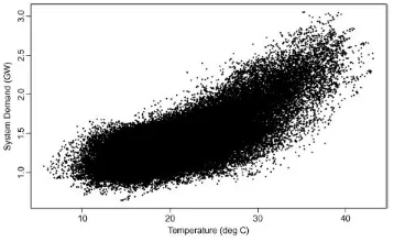
[image:32.595.202.381.480.590.2]Several studies indicate that the relationship between demand and temperature is non-linear. This non-linearity refers to the fact that both increases and decreases of temperature, linked to the passing of certain ‘threshold’ temperatures which we call the base temperature, in-crease demand. This is caused by the difference between the outdoor- and indoor tempera-ture. When this difference increases, the starting-up of the corresponding heating or cooling equipment immediately raises demand for electricity (Moral-Carcedo & Vic´ens-Otero, 2005). The base temperature is the temperature at which electricity demand shows no sensitivity to air temperature (Psiloglou, Giannakopoulos, Majithia, & Petrakis, 2009). The difference be-tween LPG and electricity on this matter is that LPG is primarily used for heating purposes so only one base temperature is required and only HDDs should be considered (Sarak & Sat-man, 2003). In order to determine this base temperature, the temperature should be plotted against the consumption. This is done in Figure 2.7 for three countries that are categorised as ‘warm’ (Greece), ‘cold’ (Sweden), and ‘intermediate’ (Germany) (Bessec & Fouquau, 2008). The y-axis gives the filtered consumption that isolates the influence of climate on electricity use. We will not go into details because it is of no importance here, the shape of the scatter plot is.
Figure 2.7: Demand versus temperature (Bessec & Fouquau, 2008)
Figure 2.8: Demand versus temperature Australia (Hyndman & Fan, 2010)
The zone where demand is inelastic to temperature is around the base temperature. As mentioned before, a decision must be made between one threshold value or two. Having two indicates a temperature interval within demand is unresponsive to temperature variations whereas one indicates a more instant transition between a regime characterised by cold tem-peratures to a regime corresponding to hot temtem-peratures. Since natural gas (LPG) is used primarily for space heating, using only HDDs is satisfactory which means that only one base temperature is required (Sailor & Mu˜noz, 1997; Sarak & Satman, 2003).
Shortcomings
A problem of the degree-days method is the determination of an accurate base temperature. In the UK for example, a base temperature of 15.5◦C is used since most buildings are heated to 19◦C and some heat comes from other sources such as people and equipment in buildings which account for around 3.5◦C (Energy Lens, 2016). However, the problem with this is that not all buildings are heated to 19◦C, not every building is isolated to the same extent, and average internal heat gain varies from building to building (crowded buildings will have a higher average than a sparsely-filled office with bad isolation and a high ceiling). Energy Lens (2016) states that the base temperature is an important aspect since degree-days-based calculations can be greatly affected by the base temperature used. When the base tempera-ture is chosen wrongly by the forecaster, this can easily lead to misleading results. However, it is difficult to accurately determine whether this base temperature is chosen wrongly since the base temperature can vary over the year depending on the amount of sun, the wind, and patterns of occupancy. Besides, when outside temperature is close to the base temperature, often little or no heating is required. Therefore, degree-days-based calculations are rather inaccurate under such circumstances.
Another important problem is that most buildings are only heated intermittently, for example from 9 to 17 on Monday to Friday for office buildings whereas degree-days cover a continuous time period of 24 hours a day. This means that degree-days often do not give a perfect representation of the outside temperature that is relevant for heating energy consump-tion. The cold night-time temperatures are fully represented by degree-days whereas they only have a partial effect (when the heating system is off at night), namely on the day-time heating consumption since it takes more energy in the morning to heat the building com-pared to a less cold night. When the difference between the outside- and inside temperature becomes bigger, as mentioned in Subsection 2.6, the starting-up of the corresponding heating or cooling equipment raises demand for energy (Moral-Carcedo & Vic´ens-Otero, 2005). Not only nights are an example but also public holidays and weekends. Moral-Carcedo & Vic´ ens-Otero (2005) made an adjustment to overcome this problem. They introduce a variable called ‘working day effect’ which represents the effect of calendar in demand of a particular day as a percentage of electricity demand on a representative day.
There are a couple of suggestions on how to overcome these shortcomings of the degree-days method. The most important one is that an appropriate time scale should be used. In the ORTEC case, the energy consumption is given once every two weeks, degree days should be gained accordingly. For example if only weekly degree days are available, those should be summed in order to make them appropriate. Besides, a good base temperature should be used.
results but the combination of the problems stated leads to the overall accuracy of the results being quite low. The results from this method can be used as an approximation of the electricity demand but do not give accurate results.
2.7
Covariates
As described in the introduction, besides time series and causal models, there is also a pos-sibility to combine them. Using covariates results in such a combined model. Taylor (2003; 2010) obtained good results for very short term forecasts in minutes or hours-ahead forecasts (Berm´udez, 2013). However, for short-, medium-, or long-term forecasts, it is important to include covariates in order to cope with for example calendar effects or climatic variables. Besides temperatures, the electricity load is also affected by working days, weekends, feasts, festivals, economic activity, and meteorological variables (Kumru & Kumru, 2015; Berm´udez, 2013; Garc´ıa-D´ıaz & Trull, 2016). Berm´udez (2013) mentions that unlike in sophisticated methodologies as ARIMA models, in exponential smoothing models the use of covariates is very recent and still infrequent.
According to Berm´udez (2013) there are some authors that use covariates in exponential smoothing models. Wang (2006) proposed to jointly estimate the smoothing parameters and covariate coefficients. The drawback of her method, however, is that she still uses a heuristic procedure to first estimate the initial conditions. Besides, she uses state space models which fall outside the scope of our research. G¨ob, Lurz, & Pievatolo (2013) refine this model by including multiple seasonalities. Just like Wang’s (2006) method, this method requires quite some mathematical skill. Another article that uses covariates in exponential smoothing is that from Hyndman et al. (2008) which introduces covariates into exponential smoothing models when they are expressed as state space models.
A method that is a bit easier, is that from Berm´udez (2013). He adds covariates for the endogenous- and exogenous effects features of which endogenous are seasonal components and exogenous are calendar effects. He does this by adjusting the Holt-Winters model by:
At=α(Yt−ωqt−It−s) + (1−α)(At−1+Tt−1) (2.36)
It=δ(Yt−ωqt−At−1−Tt−1) + (1−δ)It−s (2.37)
And the forecast now becomes
Ft+x =ωqt+x+At+xTt+It−s+x (2.38)
where Ft+x is the forecasted value x periods into the future and Yt is the observed value. ω
is the unknown coefficient of the covariate and has to be estimated together with the other unknowns. The equation for trendTt remains the same. Also a generalization to more than
one explanatory variable is also given,ωytshould be substituted by the linear combination of
the number of covariatesω0ytwhereytnow is a vector with the values of all the covariates at
starting values of the parameters and starting values. Therefore, different starting points should be used. Even then, the method does not give the optimal result that it could have done when estimating the unknowns in a better way. His R-script that is able to determine the optimal parameters and starting values, was not finished.
Berm´udez (2013) states that if too many covariates are introduced into the model, the data could be over-fitted, which produces poor forecasts. Therefore, the first step in the sta-tistical analysis should be the selection of a model which means that a selection of covariates to be used in the analysis should be made.
Concluding, there are some methods that use covariates in exponential smoothing. How-ever, these methods are either relatively difficult because of the fact that the authors use state space modelling which falls outside the scope of our research, or parameter- and initial conditions estimates that are based on heuristics or trial and error.
2.8
Artificial Neural Networks (ANN)
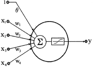
[image:35.595.207.406.390.535.2]We discussed time series-, causal models, and a combination of the two. Artificial Neural Networks however, can provide both causal- and time series models. ANNs are mathemat-ical tools originally inspired by the way our human brain processes information (Hippert, Pedreira, & Souza, 2001). Just like in a human neuron, the artificial neuron shown in Figure 2.9 receives signals through its dendrites which are the input nodes x1, ..., x4. Remember
Figure 2.9: Neuron (Hippert, Pedreira, & Souza, 2001)
the multiple regression function (Equation 2.34) and compare this to Figure 2.9. Note that the weightsw1, ..., w4 correspond with the regression coefficients b1, ..., bk. The information
processing of a neuron takes place in two stages: the first is the linear combination of the input values which is in essence the following equation:
Y =θ+w1X1+w2X2+...+wkXk (2.39)
activation functions answer the following question: ‘Some of the input switches are turned on, shall we turn on the output switch?’. In essence, an activation function determines which external variables should be taken into account. Remember that such an activation function is like multiple linear regression, but due to the nonlinear activation function, ANNs are able to model nonlinear relationships as well. Figure 2.10 shows what this logistic activation function looks like. The idea is that such an activation function is binary (0 or 1), it either fires or not.
Figure 2.10: Sigmoid (logistic) activation function
The dataset is divided into an estimation, or in this case training set, and a test set. The training set is used for estimating the parameters (weights) and the test set is used for validation (Zhang, Patuwo, & Hu, 1998). This is similar to other forecasting methods and is explained in Section 2.10.
Multilayer Perceptron (MLP)
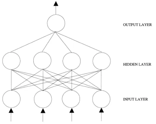
In load forecasting applications, the multilayer perceptron (MLP) architecture is one of the most popular methods, so this section focuses on that (Hippert, Pedreira, & Souza, 2001). In MLP the neurons are organized in layers. In MLP the first or the lowest layer is the layer where external information is received and the last or the highest layer is the layer where the problem solution is obtained (Zhang, Patuwo, & Hu, 1998). If the architecture is feed-forward, the output of one layer is the input of the next layer. The layers between the input layer and the output layer are called hidden layers. Figure 2.11 shows an example of such a network.
The estimation of the parameters (the weights and the biasθ) is called ‘training’ of the network and is done by minimizing for example the root mean squared error (RMSE, ex-plained in Section 2.10.
Figure 2.11: Feed-forward neural network (Zhang, Patuwo, & Hu, 1998)
ANNs have several advantages. Firstly, ANNs are non-linear whereas for example re-gression discussed in Section 2.5 is only able to model linear relationships. Secondly, it has been shown that a network can approximate any continuous function to a desired accuracy (Zhang, Patuwo, & Hu, 1998). This makes ANNs more flexible than the traditional statistical methods described earlier.
Forecasting with ANNs
As stated before, ANNs are able to solve both causal forecasting problems and time series fore-casting problems. In the first situation, the vectors of the explanatory variables are the input layer of the ANN. This makes the network quite similar to linear regression except that the network can model non-linear relationships between the explanatory variables and the depen-dent variable. The relationship estimated by the ANN can be written asy=f(x1, x2, ..., xn)
where x1, x2, ..., xn are n explanatory variables and y is the dependent variable. On the
other hand, for the time series forecasting problem, instead of having explanatory variables as input, we use past observations. This is written asyt+1 = f(yt, yt−1, ..., yt−p). Since the
number of input nodes is not restricted, it is also possible to both include past observations and explanatory variables in the model.
Nevertheless, ANNs are appealing because of their ability to model an unspecified non-linear relationship between LPG usage and external variables. This is especially appealing since we found that temperature is an external variable that strongly affects LPG usage. We do not know for sure that this relationship is linear and besides, other covariates could have some influence on LPG usage as well and the relationship (linear or non-linear) is not known yet. Therefore, despite the shortcomings of ANNs, they are definitely worth trying.
There is, however, one big condition for using ANNs: there must be plenty of data. And with plenty of data, think of thousands of observations. ANNs need this to discover patterns correctly without overfitting. A neural network is not a magic black box: it cannot discover a pattern that is not even there. Besides, when the forecaster uses a forecasting method, this choice is based on a certain amount of background knowledge. For example, when choosing Holt-Winters, this choice is based on the idea that the data has some kind of trend and seasonality. When using a neural network, the network has no such background knowledge at all; the network has all the freedom and has no restrictions which makes it extremely difficult to find patterns.
2.9
Combining forecast methods
Often, two or more forecasts are made of the same series in order to decide which one performs best. Bates & Granger (1969) argue that the discarded forecast often contains useful information. Firstly, one forecast is based on variables or information that the other forecast has not considered, and secondly, the forecast is based on different assumptions about the form of the relationship between the variables. There is, however, one condition that both forecast should meet: they should be unbiased. A forecast that consistently overestimates, if combined with an unbiased forecast, leads to biased forecasts: the combined forecast would have errors larger than the unbiased forecast (Bates & Granger, 1969).
The forecasts could be combined by averaging the forecasts but could also be combined using weights:
Ftcombined=wFtmethod1+ (1−w)Ftmethod2 (2.40) wherewis the weight given to forecasting method 1 and (1−w) the weight given to method 2. Another method of combining forecasts is by using multiple regression with the individ-ual forecast methods as input and the observed demand time series as output. This leads to the weights no longer being constrained to add to one (Deutch, Granger, & Ter¨asvirta, 1994). The advantages of this method (simple linear combining method) are that it is easy to implement and that it often yields a better forecast than either of the individual methods (Deutch, Granger, & Ter¨asvirta, 1994).
2.10
Forecast performance
In previous sections, many statements on which method performs better have been made. But how can different methods be compared on performance and accuracy?
Estimation and validation
The accuracy of a forecasting method is often checked by forecasting for recent periods of which the actual values are known (Hanke & Reitsch, 1998). Data can be held out for estimation validation and for forecasting accuracy. The data that are not held out, are used for parameter estimation (for example the α and β). The model with this parameters is then tested on the data that is withheld for the validation period. When those results are satisfactory, the forecasts for the moments in the future (of which no values are known yet) (Kuchru, 2009). Figure 2.12 visualises this estimation- and validation periods.
Figure 2.12: Estimation- and Validation period (Nau, 2017)
Withholding data for validation purposes is one of the best indications of the accuracy of the model for forecasting the future. At least 20 percent of the data should be held out for validation purposes (Kuchru, 2009). Normally, a 1-step ahead forecast is computed in the estimation period and an n-step ahead forecast in the validation period. However, in our research, we do this a bit differently. We compute a 1-step ahead forecast in the validation period with what is called a rolling horizon which means that after each 1-step ahead prediction, we do as if the information for that period becomes available (as if the estimation period becomes one step longer and the validation period one step shorter).
Performance indicators
There are several methods that calculate the accuracy of a forecast. Let us define Yt−Ft
aset, called the one-step-ahead forecast error. When comparing forecasts on a single series,
several common methods could be used; the mean absolute deviation (MAD), the root mean squared error (RMSE), the mean absolute percentage error (MAPE), and the mean error (ME).
- Mean absolute deviation (MAD) =mean(|et|)
- Root mean squared error (RMSE)
s
1
n n P t=1