Context Aware GPS Error Correction

(1)

MASTER THESIS

CONTEXT AWARE GPS

ERROR CORRECTION

Keoma Ong-A-Fat

Faculty of Formal Methods and Tools

Exam committee:

(2)

ABSTRACT

The usage of data analytics has increased greatly in the past decade, due to the increase of sensor devices producing streams of data. A major contributor in this area are the GPS systems that allow user to track and monitor the position of their devices or vehicles. And even though there are many approaches made to make these measurements more reliable, the errors produced by these measurements are still a significant issue and subject of research.

One of the most significant errors encountered in GPS data are signal multipath errors. The classification and correction of these type of errors are considered in this research. The aim of this thesis is to describe a framework that utilizes machine learning techniques in combination with the characteristics of signal multipath errors to automatically classify and correct these errors. The framework is designed to classify signal multipath errors in data from various fields of expertise by using a semi-supervised machine learning approach that uses the unknown dataset to train its classifier. By doing so the framework is applicable on a vast range of different datasets.

The framework is validated using a specific case study with data from asphalt paving projects. These projects contain the GPS trajectories of various rollers that were used during the paving process.

(3)

Table of Figure

FIGURE 1: CONSTELLATION GLOBAL POSITIONING SYSTEM ... 11

FIGURE 2: SATELLITE CYCLE SLIP ... 13

FIGURE 3: SIGNAL MULTIPATH ERROR EXAMPLE... 14

FIGURE 4: MACHINE LEARNING MODEL ... 17

FIGURE 5: MACHINE LEARNING CLUSTERING ... 17

FIGURE 6: KALMAN FILTER ... 22

FIGURE 7: ASPHALT PAVING PROJECT - PAVER ... 28

FIGURE 8: ASPHALT PAVING PROJECT - ROLLER ... 29

FIGURE 9: CURVED ROAD SECTION OF AN ASPHALT COMPACTOR ... 29

FIGURE 10: TRAJECTORY COMPACTOR COMPLETE PROJECT ... 30

FIGURE 11: ASPHALT PAVING PROJECT – OUTLIERS OVERLAY ASPARI ARCHIVE: BAM ALMERE 2016 ... 31

FIGURE 12: ASPHALT PAVING PROJECT – OUTLIERS ASPARI ARCHIVE: BAM ALMERE 2016 ... 31

FIGURE 13: SIGNAL MULTIPATH CHARACTERISTICS ... 32

FIGURE 14: CLASSIC SIGNAL MULTIPATH 1 ASPARI ARCHIVE: BAM ALMERE 2016 ... 33

FIGURE 15: CLASSIC SIGNAL MULTIPATH 2 ASPARI ARCHIVE: BAM ALMERE 2016 ... 33

FIGURE 16: UNPREDICTABLE SIGNAL MULTIPATH 1 ASPARI ARCHIVE: BAM ALMERE 2016 ... 33

FIGURE 17: UNPREDICTABLE SIGNAL MULTIPATH 2 ASPARI ARCHIVE: BAM ALMERE 2016 ... 33

FIGURE 18: SEMI-RECURRING SIGNAL MULTIPATH ERROR ASPARI ARCHIVE: BAM ALMERE 2016 ... 34

FIGURE 19: RECURRING SIGNAL MULTIPATH ERROR ASPARI ARCHIVE: TWW MARKELO 2016 ... 34

FIGURE 20: UNDEFINED ERROR 2 (COMPACTION TURNING POINTS) ASPARI ARCHIVE: BAM ALMERE 2016 ... 35

FIGURE 21: UNDEFINED ERROR 1 ... 35

FIGURE 22: SOFTWARE SYSTEM COMPONENTS ... 37

FIGURE 23: PROCESS OF AUTOMATED GPS CORRECTION ... 43

FIGURE 24: STATIC MODEL ... 44

FIGURE 25: DIRECTION AND DISTANCE FEATURES OF A POINT ... 44

FIGURE 26: ABSTRACT VIEW SYSTEM ARCHITECTURE ... 46

FIGURE 27: SYSTEM ARCHITECTURE ... 48

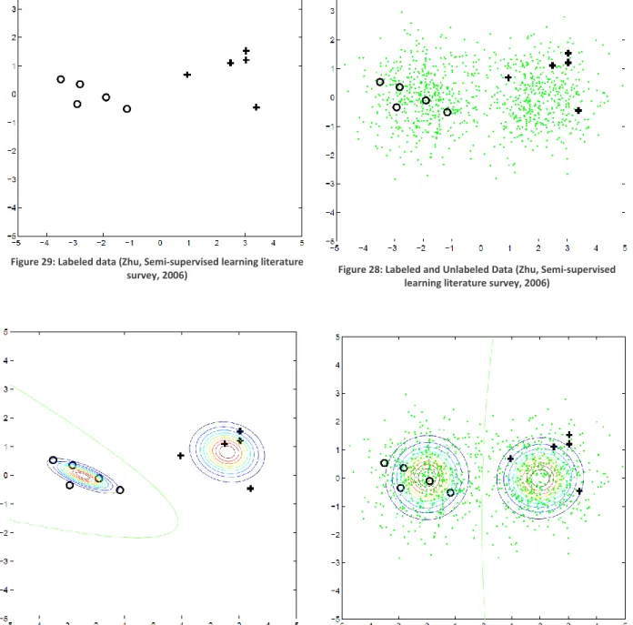
FIGURE 28: LABELED AND UNLABELED DATA (ZHU, SEMI-SUPERVISED LEARNING LITERATURE SURVEY, 2006)... 52

FIGURE 29: LABELED DATA (ZHU, SEMI-SUPERVISED LEARNING LITERATURE SURVEY, 2006) ... 52

FIGURE 30: CLASSIFICATION MODEL LABELED AND UNLABELED DATA (ZHU, SEMI-SUPERVISED LEARNING LITERATURE SURVEY, 2006) .. 52

FIGURE 31: CLASSIFICATION MODEL LABELED DATA (ZHU, SEMI-SUPERVISED LEARNING LITERATURE SURVEY, 2006) ... 52

FIGURE 32: COLLECTIVEEM CLASSIFIER ... 54

FIGURE 33: RELATED SIGNAL MULTIPATH ERROR ... 56

FIGURE 34: CORRECTION CLASSIC SIGNAL MULTIPATH ERROR ... 57

FIGURE 35: GPS MOUNTED ON A PAVER AND ROLLER NOV 2014 ASPARI ... 60

FIGURE 36: GPS TRACKER ON A PAVER ... 60

FIGURE 37: ASPHALT ROLLER PATH ASPARI ARCHIVE: BAM N316 2016 ... 61

FIGURE 38: ASPHALT ROLLER PATH MAP OVERLAY ASPARI BAM N316 2016 ... 61

FIGURE 39: BAD DATA ASPARI ARCHIVE: BAM N316 2016 ... 63

FIGURE 40: AVERAGE DATA ASPARI ARCHIVE: BAM N316 2016 ... 63

FIGURE 41: GOOD DATA ASPARI ARCHIVE: BAM N316 2016 ... 63

FIGURE 42: CLASSIC SIGNAL MULTIPATH ERROR CLASSIFIED ... 66

FIGURE 43: CLASSIC SIGNAL MULTIPATH ERROR CORRECTED ... 66

FIGURE 44: CLASSIC SIGNAL MULTIPATH ERROR CORRECTED ... 67

FIGURE 45: CLASSIC SIGNAL MULTIPATH ERROR CORRECTED (STRABAG VENAY TIRED ROLLER 1) ... 67

FIGURE 46: CLASSICAL MULTIPATH ERROR UNRECOGNIZED ... 68

FIGURE 47: CLASSICAL SIGNAL MULTIPATH ERROR UNRECOGNIZED ... 68

FIGURE 48: UNPREDICTABLE SIGNAL MULTIPATH ERROR CORRECTED (ALMERE THREE DRUM ROLLER)... 69

FIGURE 49: UNPREDICTABLE SIGNAL MULTIPATH ERROR CLASSIFIED ... 69

(6)

FIGURE 51: RECURRING SIGNAL MULTIPATH ERROR CORRECTED ... 71

FIGURE 52: RECURRING SIGNAL MULTIPATH ERROR CLASSIFIED ... 71

FIGURE 53: ALMERE THREE DRUM CLASSIFIED OVERLAY ... 72

FIGURE 54: ALMERE THREE DRUM CORRECTED OVERLAY ... 72

FIGURE 55: UNRECOGNIZED ERROR CLASSIFIED ... 73

FIGURE 56: UNRECOGNIZED ERROR CORRECTED ... 74

FIGURE 57: GPS DATA WITH CLASSIFIED ERROR SECTIONS ... 75

FIGURE 58: GPS DATA FILTERED WITH THE KALMAN FILTER ASPARI ARCHIVE: BAM ALMERE 2016 ... 75

FIGURE 59: CORRECTED SIGNAL MULTIPATH ERROR WITH KALMAN FILTER ... 76

FIGURE 60: CORRECTED SIGNAL MULTIPATH ERROR WITH CONTEXT AWARE CORRECTION ... 76

FIGURE 61: CLASSIFIED SIGNAL MULTIPATH ERROR ASPARI ARCHIVE BAM ALMERE 2016 ... 76

FIGURE 62: BAM ANKLAARSEWEG TIRED ROLLER CLASSIFIED ... 84

FIGURE 63: BAM ANKLAARSEWEG TIRED ROLLER CORRECTED... 84

FIGURE 64: BAM ANKLAARSEWEG PAVER CLASSIFIED ... 84

FIGURE 65: BAM ANKLAARSEWEG PAVER CORRECTED ... 84

FIGURE 66: BAM ANKLAARSEWEG TANDEM ROLLER CLASSIFIED ... 85

FIGURE 67: BAM ANKLAARSEWEG TANDEM ROLLER CORRECTED ... 85

FIGURE 68: BAM N316 ROVER 3 (1) CLASSIFIED ... 86

FIGURE 69: BAM N316 ROVER 3 (1) CORRECTED ... 86

FIGURE 84: STRABAG VENAY PAVER CLASSIFIED ... 94

FIGURE 85: STRABAG VENAY PAVER CORRECTED ... 94

FIGURE 86: STRABAG VENAY TANDEM ROLLER CLASSIFIED ... 95

FIGURE 87: STRABAG VENAY TANDEM ROLLER CORRECTED ... 95

FIGURE 88: STRABAG VENAY TIRED ROLLER CLASSIFIED ... 96

FIGURE 89: STRABAG VENAY TIRED ROLLER CORRECTED ... 96

FIGURE 90: STRABAG VENAY TIRED ROLLER (2) CLASSIFIED ... 97

FIGURE 91: STRABAG VENAY TIRED ROLLER (2) CORRECTED ... 97

FIGURE 92: TWW MARKELO ROVER 1 CORRECTED ... 98

FIGURE 93: TWW MARKELO ROVER 1 CLASSIFIED ... 98

FIGURE 102: BAM ALMERE PAVER CLASSIFIED ... 103

(7)

FIGURE 104: BAM ALMERE THREE DRUM CLASSIFIED ... 104

FIGURE 105: BAM ALMERE THREE DRUM CORRECTED ... 104

FIGURE 106: BAM ALMERE TANDEM CLASSIFIED... 105

FIGURE 107: BAM ALMERE TANDEM CORRECTED ... 105

FIGURE 108: TIEL PAVER 1 CORRECTED ... 106

FIGURE 109: TIEL PAVER 1 CLASSIFIED ... 106

FIGURE 110: TIEL PAVER 2 CORRECTED ... 107

FIGURE 111: TIEL PAVER 2 CLASSIFIED ... 107

FIGURE 112: TIEL TANDEM 1 CLASSIFIED ... 108

FIGURE 113: TIEL TANDEM 1 CORRECTED ... 108

FIGURE 114: TIEL TANDEM 2 CLASSIFIED (ROTATED 45 DEGREES) ... 109

FIGURE 115: TIEL TANDEM 3 CORRECTED (ROTATED 45 DEGREES) ... 109

FIGURE 120: TIEL TIRED ROLLER CORRECTED ... 110

FIGURE 121: TIEL TIRED ROLLER CLASSIFIED ... 110

FIGURE 122: TIEL BABY TANDEM CORRECTED ... 110

(8)

1. INTRODUCTION

GPS equipped devices have proven their usefulness in various fields in life such as navigational, tracking and even behavior analysis applications. There are many areas that would profit from increased accuracy and increased reliability of their GPS measurements. One of these areas where the precision of GPS measurements is crucial, is the asphalt paving industry. To analyze asphalt paving projects and improve the compaction process, the projects are visualize based on the measured GPS trajectories of the machines. Based on these visualizations the projects are analyzed. Any inaccuracy in the measurements directly translates into the analysis results, which can lead to incorrect conclusions and finally to costly erroneous management faults.

There are several causes of GPS measurement errors of which the most significant are signal multipath errors, Los of Signal errors, Ionosphere errors, Satellite orbit errors and Satellite clock errors (Braasch, 1996).

These errors are filtered and corrected during the measurements by the GPS equipment up to a certain degree but cannot be removed completely (Macdoran, 1996). In most cases

post-processing of the GPS data is the most optimal solution, which is done by experts who are familiar with the context of the measurements and can by their expertise knowledge classify and correct the data manually. Since this is error prone and labor intensive, an automated solution is required that will automate this process, removing the necessity of experts and the manual filtering process.

To achieve fully automated post-processing of GPS data, machine learning techniques can be used that allow for autonomous recognition and correction of incorrect measurements based on the patterns found in the data. By doing so, the contextual information and understanding of the datasets, as used by experts, will be directly derived from the data and applied to detect and correct measurement errors.

Every dataset has specific characteristics that are determined by the movement of the receiver. Measurements of traveling vehicles are more stable than measurements of wildlife animals and have different measurement outliers, because of the different measurement surroundings. These characteristics describe the context of the measurements that provide additional information that can be used to correct the data.

The effectiveness of such an approach that uses this information depends on the consistency of the data, the distinctiveness of the errors and the metrics used to classify and correct them.

(9)

The questions that need to be answered to provide a solution for the described problem are as follows:

1. What are the effects of signal multipath errors on the GPS measurements? 2. How can you recognize the context of GPS measurements using machine learning

techniques?

3. How do you automatically correct signal multipath errors based on their context in GPS datasets?

4. How can signal multipath errors be recognized and corrected during real-time measurements?

The obtained solution will be validated using datasets from various asphalt paving projects that contain the GPS measurements of the used vehicles.

The classification of the erroneous points will be validated using several machine learning classifier performance indicators that describe several aspects of the classification accuracy (Powers, 2011). The classification will be done by a using a pre-defined testing set that contains a combination of valid and erroneous points.

The complete framework will be validated by classifying and correcting the complete asphalt paving datasets. A geographical map overlay on the data will also be provided to bring the data and the significance of the corrections into context.

The research questions will be answered in the following sections of this thesis. Firstly, the signal multipath errors are considered, their characteristics and influence on the data will be analyzed. Secondly, the machine learning techniques needed to detect and classify these errors in the data are discussed. Thirdly, the correction of these errors, based on their influence on the data, are described. Fourthly, the applicability of the proposed solution for real-time

measurements are considered. And finally, the proposed solution is described and validated in the last section of the thesis.

(10)

2. BACKGROUND INFORMATION

This section will describe background information of the techniques and terms used throughout this thesis. The aim of this section is to make the reader acquainted with the subject and the domain-specific knowledge needed to understand the provided architecture and solution of this research.

Firstly, the Global Positioning System is described, followed by the applicational areas of GPS, followed by an introduction to machine learning and the Kalman Filter.

2.1 Global Positioning System

2.2.1 GPS Constellation

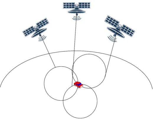
The Global Positioning System (GPS) is a system that is used in various applications to locate the position of objects on earth. The combination of dedicated satellites located at 20 000

kilometers above the earth’s surface and the GPS receivers on earth allow for accurate location estimation of GPS receivers. The constellation of the currently used Global Positioning System is given in Figure 1. The figure shows three satellites, moving in an orbit around the globe and a GPS receiver, represented by the car.

(11)

When a satellite sends it current position and time-stamp to the receiver it can determine the

geographical location that could be reached by the satellite’s signal by comparing the time -difference of the sending and receiving moment of the signal. It can then determine the radius of the area that was reachable for the satellites signal as shown in Figure 1. When this is done for three individual satellites, the intersections of these radians will determine the actual location of the receiver. The receiver can in this manner calculate its current position if it has a direct line of sight with at least three satellites. The accuracy of the location estimation is determined by various biases and errors that are encountered during this process, which are described in the following sections.

(12)

2.1.2 Biases

There are three categories of biases that can be created that can negatively influence the accuracy of the location prediction of the receiver, namely; Satellite biases, Station biases and Observation dependent biases (Wells, 1987).

Satellite biases are caused by inconsistencies in the actual location of the satellite and the location information about the satellite or clock errors at the satellite’s side (Wells, 1987).

These biases cause a misinterpretation at the receiver’s side about the actual location of the

satellite and will cause it to make a wrong estimation of the location of the radius that the satellites signal can reach, thus estimating a wrong geographical location for itself.

Station biases are caused by clock biases of receivers and inaccuracies in the position

information of the control stations (Wells, 1987). Biases in the clock information of the receiver makes the receiver to calculate an incorrect time difference between the time the satellite signal was send and the time that it was received at the receiver’s side. This will also result in an

incorrect estimation of the radius the satellites signal could have reached, because of the incorrect transmission time. Invalid information about the actual location of control stations will result in incorrect offset corrections on the estimated location of the receiver, also resulting in incorrect location prediction.

Observation dependent biases are biases created by errors of the signal propagated by the satellite. These errors can be caused by ionospheric delays, tropospheric delays or carrier beat phase ambiguity (Wells, 1987).

2.1.3 Errors

(13)

Figure 2: Satellite Cycle Slip

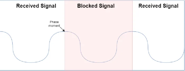
Another error encountered are phase center movement errors. These errors are caused by the wrong assumption that the signal reaches the receiver at the center of its signal phase. When the signal reaches the receiver at a different point of its phase, an incorrect estimation of the distance calculation will be made.

Next to the phase center movement errors are observational errors. These are caused by the equipment that is only capable of observing the received signal from the satellite up to a certain degree of accuracy. These errors are often compensable by cancelling them out against each other based on the different signals received from the satellites.

The final error described is the error with the greatest impact on the accuracy of GPS

measurements, which is the signal multipath error (Macdoran, 1996). These errors are caused by signals reaching the receiver indirectly through reflecting objects, thus influencing the position and direction of the GPS signal, causing an incorrect estimation of the location of the receiver as shown in Figure 3. The sender perceives the receiver to be position behind the reflecting object, causing a change in direction and distance between the erroneous

(14)

Some signal multipath errors can be corrected with coded based signals, such as pseudo-range messages. When signal multipath errors occur and there is still a direct signal that can reach the receiver, a distinction can be made between the direct signal and the multipath signal, because coded signals are characterized by their chip length (Wells, 1987). Whenever the multipath signal exceeds this chip length, it can be distinguished from the direct signal and discarded. When the additional signal multipath traveling path is smaller than the chip length in regard of the direct signal or the direct signal does not reach the receiver, this error cannot be corrected in real-time measurements.

The effects of signal multipath errors on the perceived trajectory of the receiver depends on the stability of the reflecting objects. Whenever the reflecting object moves, the effects on the directional and positional change of the perceived trajectory varies greatly. When the reflecting object is static, the differences in the actual and the perceived trajectory of the receiver are constant and predictable.

Because of the significance of this type of error and the absence of a solution that works for every type of GPS system, the signal multipath error has become the main subject of this research. All other errors can be compensated or their effects can be significantly reduced during the measurements of the data, however signal multipath errors are unpredictable and undetectable in most cases, which makes them the most interesting and impactful error encountered during GPS measurements.

The following sub-section will describe the most common applicational areas of GPS measurements, which will put the usage of GPS in context in combination with their error tolerance.

(15)

2.2 Relevant Applications

Since GPS satellites are freely available to users around the globe, a vast community of users has been established with many varying applications of this positioning system. This section will describe some of the areas in which GPS is applied and their fault tolerance that is accepted by them.

One of the fields in which GPS is applied is the field of land surveying and mapping. This field includes cadastral surveying, geodetic control, local deformation monitoring and global deformation monitoring. Every of the afore mentioned areas require relative accurate measurements, however some require more detail than others. Where cadastral surveying requires an accuracy of 10e-4, global deformation monitoring that monitors plate tectonics, require an accuracy of up to 10e-8 (Wells, 1987).

A very popular field of application are land applications that use GPS for positioning and navigational purposes. These applications require less accuracy where an error margin of a meter is tolerable, depending on the specific application (Wells, 1987).

In airborne surveying and mapping applications an accuracy between 0.5m up to 25m is tolerable, which can be easily met with GPS (Wells, 1987). Also, aerial photogrammy, airborne laser profiling and airborne gravity and gravity gradiometry require less GPS accuracy and are more fault tolerant.

(16)

2.3 Machine Learning

2.3.1 Why Machine Learning?

Machine learning is a technique that is used more and more in various fields. This is not without reason. As the usage, traffic and storage of data increases, the analysis and utilization of this data becomes more labor intensive and time consuming.

Machine learning provides adaptive algorithms that allow for the algorithm to make decisions based on a specific scenario. This makes machine learning dynamic in nature compared to traditional static hard coded algorithms. This is crucial in the current developments, because the amount of data that needs to be analyzed varies more and more and creating tailor made solutions for every scenario is unthinkable.

Machine learning techniques provide a solution for this problem, whereby the algorithm learns about the features of a specific dataset and based on the relationships between these features changes its choice making policy. This provides for tailor made solutions for a fast variety of different datasets without the need of adapting the algorithm or any other human interaction.

Some of the areas where machine learning is used are spam filters, face recognition and language recognition programs. Spam filters for example, must decide whether a specific incoming mail belongs to the valid mail category or must be classified as unwanted spam mail. Each user has different contact types and therefore different types of incoming mails. Where a specific mail can be considered spam for one user, the same mail will be a good mail for another. A spam filter therefore adapts its selection algorithm based on the user’s behavior to classify spam more accurately according to that specific scenario.

There are two main divisions in machine learning, which are supervised and unsupervised machine learning. They both work a bit different and are used for different purposes.

Supervised machine learning is used to classify data attributes from a dataset into given classes. It uses a training set with labeled data that is already classified to find the relationships

(17)

Unsupervised machine learning is used to cluster data. With this type of machine learning there is no class information known before hand and the relationship between the data points is examined to cluster them in distinct groups as shown in Figure 5. This can provide additional information about the relationship of the data points, however since there is no knowledge about classes, the classes of the data points cannot be determined. It is mostly used in the exploratory phase of data analysis, where the similarities of the clustered groups are analyzed.

Figure 4: Machine Learning Model

(18)

There are many implementations of various machine learning algorithms but they work

basically in the same way. Firstly, important features are selected from a training dataset, then the relationship between these features are examined, after which the accuracy of these predictions are tested on a testing set with labeled data and then a model is created based on the found relationships. This model is then used to classify new incoming data assuming it contains the same relationship in the data as the data used to create the model.

The following section will discuss these various aspects of the machine learning process.

2.3.2 Training and Testing

A very important step in machine learning is the feature extraction phase. To learn the

algorithm to recognize the specific features of a data attribute that belongs to a specific class, the algorithm must have knowledge about these features and their relationships regarding the different classes.

To do so, the features of the data attributes are manually extracted from the data. Considering the analysis of GPS data, features to be analyzed could consist of directional information, speed and geographical locations. Every measured point contains these features and these features are used to classify the point to a class established by the user.

One could think of an example whereby the speed and angle change of GPS points can be used to classify the moments a driver was making dangerous turns. Here the relationship between the speed and the angle change attribute will determine the classification of a point belonging to the dangerous or the save driving class.

The first step for a machine learning algorithm is describing these features and labeling the points manually, which will provide the algorithm information about the data features and the class to which a point containing those features belongs to. This information is stored in the training set, which is used to train or to teach the machine learning algorithm the relationships between the data features and the assigned classes.

After this relationship is established, it is tested with a testing set. This testing set is also a dataset with pre-labeled data, whereby the data attributes are already classified. Often the testing set is a part of the training set. This is significant, because the relationship established by the algorithm is validated by removing the labels from the testing set, labeling this set based on the established relationship and validating the results with the original testing set.

In some cases, the part of the labeled data that is used for training and the part that is used for testing can produce different results. Therefore, often methods like K-Cross Validation are used to randomly change the portions used for training and testing to find the best working

(19)

2.3.3 Classification

After the best performing relationship is established as the classification model, new data attributes can be classified based on their features. To do so, the features of every new data attribute are extracted and examined by the model. Depending on the type of classification algorithm used the data attribute is assigned to a class. The models and their strengths and weaknesses are explained in the Context Aware Classification section.

2.3.4 Validation

Machine learning techniques are used in various areas of expertise and provide solutions by increasing the entropy about unlabeled data attributes using the created model. Understanding the performance of the created model is crucial for the interpretation of the results and for the selection of the model that suits best for the given problem case.

Understanding the performance of machine learning classification models is done by measuring the classification performance indicators. There are several features of the classification that are considered that collectively represent the classification performance of the model. All these

features show a different aspect of the model’s performance and therefore different models

with different distributions can be suitable for different problems. The most commonly used indicators are described in the following section.

The indicators that are used are all deduced from the correct hit ratio of the classifier. To understand them, the concept of true positives, false negatives, false positives and true negatives must be understood. Their definitions are as follows.

Consider a set of unlabeled data that must be labeled by the classifier. Whenever an unlabeled data instance is a positive instance and is labeled as such, it is called a true positive

classification. Whenever a data instance is a positive instance but is labeled as negative, it is called a false negative, since it is falsely classified as a negative instance. The four classification possibilities are given below.

• True Positive: A positive data instance that is classified as positive.

• False Positive: A negative data instance that is classified as positive.

• False Negative: A positive data instance that is classified as negative.

• True Negative: A negative instance that is classified as negative.

C1 C2

C1 True Positive False Negative

(20)

The performance indicators are all based on the relationships between these mentioned hit ratios of the classifier. The most commonly used performance indicators are given in the following list, where more detailed descriptions can be found in (Powers, 2011).

Definitions

True Positive Rate (Sensitivity / Recall) TPR = TP/P = TP / (TP+FN)

False Positive Rate (Fall-Out) FPR = FP/N = FP / (FP + TN)

Positive Predictive Value (Precision) PPV = TP / (TP + FP)

F1-Measure F1 = 2TP / (2TP + FP + FN)

Accuracy ACC = (TP + TN) / (TP + FP + FN + TN)

The true positive rate, sensitivity or recall indicator indicates the performance of the

classification model in respect of classifying instances that are positive. In the given example, it reflects the performance of detecting the positive data instances from the unlabeled data. Is shows how many of the positive instances were classified as such.

The positive predictive value or precision reflects the precision wherewith the model can classify instances belonging to the positive class. It reflects the relationship between the

correctly and incorrectly positively classified instances. In other words, it shows the percentage of correctly classified positive instances in respect of all classified instances.

The F1-Measure is the harmonic mean of precision and sensitivity (Powers, 2011). It gives a weighted average between the precision and recall. The result will vary between 0 and 1, where 1 is the best reachable value.

The accuracy reflects the relationship between the correctly and incorrectly classified instances. It is the result of all correctly classified instances over all classified instances, giving a

percentage of the accuracy of the classification model.

These different indicators together give a clear view on the performance of the classifier in respect of correctly classifying positive, negative and all instances. Some models may be very accurate in detecting positive instances, whereby they do not have a high overall accuracy. Using this approach to validate classification models, different strengths and weaknesses of the models can be evaluated.

P Positive Instances FP False Positives

N Negative Instances TN True Negatives

(21)

2.4 Kalman Filter

Aside from machine learning techniques, other filtering techniques such as the Kalman Filter are often used in relationship with GPS based data. In this research, the Kalman Filter is used for correction purposes were no error information is available. The following section will introduce this filter, how it works and why it is usable.

The Kalman Filter technique is a recursive solution to the discrete data linear filtering problem (Kalman, 1960).

Filtering problems occur when erroneous data measurements are recorded. These errors can occur because of faulty equipment and various other circumstances. These circumstances may not always be known and the effects on the measured data can be unpredictable.

To obtain more reliable and accurate data, these erroneous data measurements are either removed or replaced by prediction on the actual correct values of the measurements. To make these predictions a model of the actual world is created, as described in the machine learning section, that will simulate the measurements and by doing so can correct or filter the erroneous data. Creating a model that can do so requires additional knowledge about the measurements for which often a set of previous measurements are used.

The Kalman filter finds its strength in its ability to predict new measurement values without any prior knowledge about the dataset, except the previous measurement and their error margin. This ability makes it very useful in cases where there is insufficient knowledge to produce an accurate model of a system (Welch, 1995).

(22)

Figure 6: Kalman Filter

A Kalman filter uses two significant values to predict the upcoming state of a system. Those are the previous measurement values and the measurement noise values (Welch, 1995). The measurement noise values can also include process values. The Kalman filter considers a

measurement and the noise that influences the result of that measurement. By considering this noise a prediction is made for the upcoming value, including a noise value for the newly

predicted measurement value. These values are compared with the actual measurement and their noise values. A weighted average is taken between the predicted and measured value in which the noise variance is minimized. By doing so, the new value has a smaller noise value than the predicted as well as the measured value. This results in a smoothing of the data by making a compromise between the actual measured data, which you suspect to be erroneous, and the predicted data, which you suspect also not to be perfect. This process is recursively repeated, whereby the noise value of the last chosen value is used for the prediction of the next value. This value includes the behavioral information of the system in the prediction of the next value, without having knowledge of earlier states of the system.

By doing so, the noise value quickly converges to a minimal and more accurate predictions can be made for upcoming measurements, with only the information of the previous value and its noise parameter.

(23)

2.5 Conclusions

The previous section has introduced the relevant topics of this research and their background information.

The data that is used during this research consists of GPS measurements and is aimed at detecting the signal multipath signals in such datasets.

There are many fields of expertise that would profit the increased accuracy and reliability when signal multipath errors can be corrected as described in the relevant applications. The accuracy needed from GPS measurements can vary per application field and depends on the specific application of the data.

To recognize the signal multipath errors, machine learning techniques will be used, which are able to automatically classify such patterns in the datasets by learning the relationship between the data attributes of the dataset and by doing so can predict the type of class an unlabeled point belongs to, based on its attributes.

The part of the correction of the points will be done using a Kalman filter, which is shortly described in this section. This filter can predict upcoming data points without knowledge of previous data points, except the last point and its noise value, which is useful to predict missing segments and erroneous points without additional information.

(24)

3. RELATED WORK

The aim of this research is to provide a framework to classify erroneous GPS measurements based on their context using machine learning techniques. As well as GPS filtering as machine learning techniques are well known subjects of research and are extensively covered in many scientific works. The following section will describe related work on GPS filtering techniques and machine learning techniques that are related to this study.

3.1 Real-time correction

As described in the 2.1.3 Errors section, signal multipath errors contain several distinct aspects in their effects on the measurements as well as on the GPS signal itself. The first line of defense against signal multipath errors is found in detecting and handling these errors in the received satellite signal by the GPS receiver.

In (Georgiadou, 1988), the ability to identify signal multipath errors by looking at dual phase signals of GPS carrier phase observations is described. This approach requires dual frequency receivers and the use of carrier phase measurements.

The research of (Townsend, 1995) describes a method using the Multipath Estimated Delay Lock Loop (MEDLL) to reduce the effects of multipath errors within the receiver’s tracking loop

for single frequency receivers. It showed significant improvements of accuracy in carrier phase measurements. The application of this technique has also shown its effectiveness on C/A code pseudo range measurements.

Another technique used is the Signal-to-Noise-Ratio multipath based error correction technique as described in (Axelrad, 1996). This technique uses the differences in amplitude perceived from the signal-to-noise-ratio to create a multipath correction profile for the perceived error. This technique can also handle changing environments for carrier phase measurements.

(25)

3.2 Post Processing

Another approach in dealing with signal multipath errors is not on the received signal level but on the effects of the error on the measurements registered by the receiver.

The filtering of GPS measurements is application specific, because the data produced per application can vary greatly in nature. Therefore, mostly general filtering techniques are used that can smooth out the data or experts manually correct the datasets, using their additional understanding of the datasets.

In (Liu, 2010), a two-filter smoothing algorithm is described to increase the accuracy of land navigation. This paper describes the use of a Kalman Filter in combination with a Rauch-Tung-Striebel Filter to enhance navigation in urban environments. These urban environments result often in signal loss and signal multipath errors due to the urban canyons of high buildings with reflecting materials. The use of these filters proved to be especially useful in cases of loss of signal errors.

Several different implementations and adaptations of the Kalman Filter have been used to correct errors in GPS measurements as described in (Mohamed, 1999). The two significant approaches described are the Innovation-based Adaptive Estimation (IAE) and the Multiple-Model-based Adaptive Estimation (MMAE) Kalman filters. These techniques are adaptive in the sense that they change the weights of the covariance and noise variables to increase or

decrease the importance of the estimated value of the filter in relation with the measured value. These techniques proved to provide a greater correction accuracy than a classic Kalman Filter.

(26)

3.3 Machine Learning

The difference between the earlier smoothing and correction approach and machine learning is found in the additional information that is retrieved from the to be analyzed dataset. With machine learning techniques, the behavior pattern of the system can be more accurately

predicted, because of the additional information provided by the system. This information gives an advantage when it comes to interpretation and processing of GPS data that can greatly increase the error detection and correction of the data.

One of the area’s where this information is used is in the classification of measurements

surroundings in GPS tracking applications. As described in (Ziedan, 2012), the quality of GPS measurements can be greatly influenced by their surroundings, since every type effects the received signal strength and signal multipath occurrences. In this research, the received signals in the C/A code GPS measurements are used to detect signal multipath signals using machine learning techniques. The signals are classified as signal multipath errors based on the

characteristics of classic signal multipath errors and the overall signal behavior of all measured signals. By determining the signal multipath signals received, the surroundings in which the measurements were done can be determined, which determines the correction algorithm that is used to correct the data accordingly.

The relevance of this research lies in the approach of differentiating GPS data by means of machine learning techniques. Even though the described research classifies GPS signals instead of geographic points, the approach is like the research described in this thesis in the sense that is also tries to deal with signal multipath errors using machine learning techniques.

In (Xu, 2010), pattern recognition techniques are used to identify several different travel modes from data derived from different traveling subjects. Here, fuzzy variables were used to classify tracking measurements into one of the selected travel modes using pattern recognition. Also, speed related variables were used, considering the traveling speed of the receivers used, which is comparable to the distance feature used in this thesis.

The research done in (Zheng, 2008), takes this a step further, whereby it also includes

directional changes as features for the data attributes to be classified. This research also aims at identifying users traveling modes, however it distinguishes itself in the set of features used to characterize the GPS data and the machine learning techniques used to classify the

measurements in different traveling modes.

(27)

Moreover, earlier research has not focused on identifying signal multipath errors based on their influence on the geographical location measured by the receiver. As seen with the previous works, signal multipath errors are not considered or used to increase the accuracy of the measurements. Classifying signal multipath errors based on their positional and directional influence on GPS measurements is a new field of research.

Also, none of the earlier works attempt to correct the GPS measurements based on known error characteristics. All erroneous measurements are considered similar and are treated in a similar manner as loss of signal errors.

3.4 Conclusions

As seen in the described earlier works, GPS errors are studied from different angles and with different approaches. However, specifically targeting signal multipath errors based on their characteristics found in the geographical changes produced by them is a new concept. Also, using this information to correct the detected errors has not been done before.

Previous works do give good information about the data features of GPS measurements that are useable for data extraction, which is an important aspect of the solution proposed in this research.

(28)

4 PROJECT DESCRIPTION

The solution provided in this research is applicable in various fields of expertise but will be validated using a specific case study with data from asphalt paving projects. The following section describes the background information of these projects to understand the data they provide and the specific errors that are subject of this research.

4.1 Description Case Study

The data used in this study is derived from various asphalt paving projects. An example of such a project is given in Figure 7 and Figure 8. Here you can see an asphalt paver that is laying the

asphalt on the road’s surface and an asphalt roller that is compacting the asphalt to achieve the optimal density of the asphalt mix. Every machine is equiped with a dedicated GPS tracker that is recording their position every second.

This produces datasets which are shown in Figure 9 and Figure 10.

The datasets consist of latitude and longitude coordinates given in the WGS84 geodetic datum format, combined with a date and timestamp indicating the time of measurement. The GPS positions are recorded for every second and stored in csv files.

N52°22'25.00104"; E5°11'57.45511"; 41.973; 2-11-2016 5:53:06.000

(29)

The measurements reflect the trajectories of asphalt compactors that move up and down in a repetitive manner. The compactors are restricted in their turning angles and in their maximum speed, which directly translate in consistent data with limited angle changes and distance variations between the measured points.

A sample of a dataset is shown below in Figure 9, where the green lines reflect the machine paths of the compactor.

(30)

As shown in the figure, most of the movements of the compactor are regular and do not move out of the boundaries of the road. The movements are lightly curved and are consistent in direction over the road section. This is the general pattern for the movements of the asphalt compactors during an asphalt paving project. The data of the trajectories of a compactor of a complete project is shown in Figure 10.

Figure 10: Trajectory Compactor Complete Project

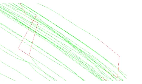
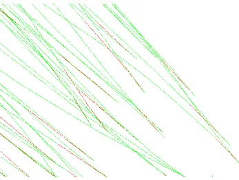
While the data of most road sections seem consistent and accurate, there are several sections found in the datasets that contain outliers. Some of these outliers can be recognized as signal multipath errors, where some other outliers have an undefined origin.

These outliers are also visible in Figure 11 and Figure 12. These figures strongly illustrate the danger of the misinterpretation of erroneous data. Because of the satellite overlay, it is clearly

visible that some path sections are visualized out of the roads boundaries, which isn’t directly

clear without the overlay. This signifies the importance of identifying such sections and correcting them before the interpretation of the visualization takes place.

(31)

Figure 11: Asphalt Paving Project – Outliers Overlay ASPARi Archive: BAM Almere 2016

(32)

4.2 Classic Signal Multipath Errors

The first error considered in this section are classical signal multipath errors.

The classic signal multipath errors are the signal multipath errors that have four distinct error angles that are related to each other. Signal multipath errors are caused by obstacles that block the signal of the GPS transmitter to directly reach the receiver, whereby it is reached through a reflecting object as described in 2.1.3 Errors. When this object is consistent, the adaptation of the location of the receiver is consistent in respect of its actual path. This phenomenon is shown by Figure 3. Figure 13 shows the effect of this error on the actual measurements.

Figure 13: Signal Multipath Characteristics

Typical about this error are the changes in the direction at α1, β1, β2 and α2. These angles are

each other’s inverses where; α1 ≈ -β1, β1 ≈β2 and β2 ≈ -α2.

Aside from the relationship in the angles, another relationship is found in the distance between the two points of the first outlier indicated with c1 and the distance between the points of the second outlier indicated with c2. This distance is approximately equal but inversed in direction.

A third notable attribute of classic signal multipath errors is the consistency of the distance between the points between the start and ending of the error. The measured points behave similarly to valid measured points, except their location has an offset, which is determined by the distance between the receiver and the reflected object and given by α1 and c1.

When a set of points contain these attributes, the whole set is recognized as a classic signal multipath error.

(33)

4.3 Unpredictable Signal Multipath Errors

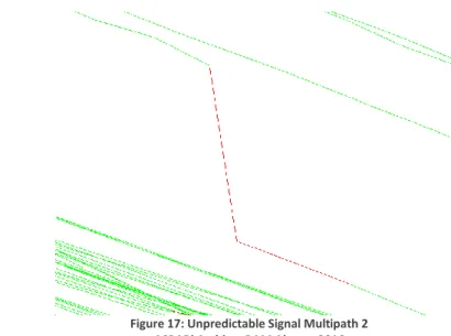
Unpredictable signal multipath errors are signal multipath errors that have a starting point but no recognized ending point. These errors can occur when the GPS receiver is moving for a longer period behind an object. Even though the outliers created when the receiver moves behind the blocking object can be detected, the end of the error is either not present or not easily recognized. This often happens when the blocking object moves simultaneously with the receiver and eventually cancels the signal multipath error.

Instances like this are still classified as signal multipath errors when they have the

characteristics of the beginning of a signal multipath error. It must have a distinct change in direction and distance between the points and the points following must maintain the regular motion of the receiver. Some examples of these errors found in the data are given by Figure 17 and Figure 16.

Figure 14: Classic Signal Multipath 1 ASPARi Archive: BAM Almere 2016

Figure 15: Classic Signal Multipath 2 ASPARi Archive: BAM Almere 2016

Figure 16: Unpredictable Signal Multipath 1 ASPARi Archive: BAM Almere 2016

(34)

4.4 Recurring Signal Multipath Errors

Recurring signal multipath errors are signal multipath error segments that are encountered more often at a specific geographical location. This is caused by static objects that block the satellite signal at that specific location. One example of a semi-recurring signal multipath error is given in Figure 18. Here it is visible that at the same location a signal multipath error occurs at different moments in time. However, this is not an absolute recurring signal multipath error, because there are other moments the compactor passes the same location, without

experiencing a signal multipath error.

The semi-recurring signal multipath errors that were found are most likely caused by moving objects that were present only at a specific time during the project. Objects like asphalt trucks and other machinery could cause such errors.

The project data also contained recurring signal multipath errors with irregular outlier characteristics as shown in Figure 19. These recurring signal multipath errors are consistent throughout the whole paving process and indicate the presence of a bridge, trees or other static objects capable of blocking the signal. Noticeable about these errors is the inconsistency of the angle and distance changes at these points. These variations indicate that the reflecting

object by which the receiver receives its signal is inconsistent compared to the receiver’s

position. Even though these errors are signal multipath errors, they do not have the classic signal multipath error characteristics and their change in direction and change in distance cannot be predicted.

Figure 18: Semi-recurring Signal Multipath Error ASPARi Archive: BAM Almere 2016

(35)

4.5 Undefined Errors

As described in the recurring signal multipath problem, several classified outliers do not conform to the predictable signal multipath behavior and are therefore defined as undefined errors. All errors that do not contain the signal multipath characteristics in direction and distance change are classified as undefined, even though they could well be signal multipath errors.

For the asphalt paving dataset, a specific kind of error is encountered caused by the direction changes of the compactors during asphalt compaction. The rollers move up and down the asphalt in a repetitive motion, which causes inverted directions at their turning points. These points are outliers and invalid behavior according to the system as shown in Figure 20, even though considering the context of the data this behavior is valid.

Figure 21: Undefined Error 1 ASPARi Archive: TWW Markelo 2016

(36)

4.6Conclusion

(37)

5 SOFTWARE ARCHITECTURE

The following section will describe the implementation of the solution of the given problem. The section begins with the problem description from which the requirements are derived. Based on the requirements of the system an architectural design is created and described and the section is closed with the implementation of the design.

After the description of the system architecture, more light is shed on specific components of the system that are relevant to the described framework.

5.1 Problem Description

As described in this research, the main objective is to automatically classify and correct signal multipath errors in GPS datasets. To achieve this purpose, a framework is designed that provides a solution that is usable in various fields of expertise. The following section will describe the requirements of this framework. The implementation of this framework used in this research contains those requirements but in addition also fulfills the requirements for the system needed to validate the framework as shown in Figure 22.

(38)

As shown in Figure 22, the framework functionality includes the classification and correction of GPS data points. The problem description of this research describes the difficulty of manually detecting and correcting signal multipath errors in GPS data.

To solve this problem, the framework must be able to automatically detect signal multipath errors in a dataset. This can only be done by a certain degree of knowledge of the dataset, wherewith the distinction can be made between valid and invalid points, since every dataset has different correct relationship between measured points. A distance and angle difference between two measured points that describes normal behavior in one dataset can describe erroneous data in another.

In addition, the framework must be able to correct the detected erroneous sections in the data, compensating for the detected error. It must be able to correct signal multipath errors and so improve the overall accuracy of the measurements.

But before the data can be classified and corrected, the data must first be read be the system. This functionality of the system is application specific and will differ for every type of data file and format that the user provides. This part of the system must be able to read the latitude and longitude position and the time of the measured data point, which are the three metrics that are used by the system. Also, the data must not contain missing measurement segments in the data. In this research, the import component of the system must be able to read the latitude, longitude and timestamp of the measurements from a .csv file in WGS84 format.

After the processing of the data, the results must be visible to the user. This can be done by exporting the results into a new datafile containing the corrected data points or by visually expressing the results. For this research, the latter option has been chosen, since a visual representation is easier to analyze and provides more insight in the data for human

interpretation. Therefore, the system must be able to visually represent the datafiles that are fed to the system must be able to visually represent the processed dataset.

(39)

5.2 Software Quality and Requirements

Functional Requirements

The described functionalities of the system can be translated in concrete functional

requirements that describe what the system must be able to do. Table 1 gives a description of these requirements, based on the previously described purpose of the system.

#

Requirement

Description

IMPORT FUNCTIONALITY

R1 Import GPS data from .csv files The user must be able to import GPS data files with latitude, longitude and time information from .csv files into the system.

R2 Correct missing segments The user must be able to remove or correct missing

data segments from the imported dataset. FRAMEWORK FUNCTIONALITY

R3 Automatically classify signal multipath errors in GPS datasets

The user must be able to automatically label signal multipath error points in the dataset as such. Without any additional user input, except from the dataset itself, the user must be able to receive signal multipath errors in the dataset, identified by the system.

R4 Automatically correct signal multipath errors in GPS datasets

The user must be able to automatically correct signal multipath errors in the dataset. Without any

additional user input, except from the dataset itself, the user must be able to receive the corrected data, corrected by the system.

VISUALIZATION FUNCTIONALITY

R5 Visualize signal multipath errors in a GPS dataset

The user must be able to view the signal multipath errors detected by the system on a map.

R6 Visualize corrected data in a GPS dataset

The user must be able to view the corrected data points, corrected by the system, on a map.

(40)

Non-Functional Requirements

The architecture designed must possess several software quality characteristics (ISO/IEC, 25010:2011) to achieve its described purpose. The considered quality characteristics of the architecture are given below with their motivation and relevance.

The summary of these requirements is given in Table 2.

The first characteristic of the system is functional suitability. This means that the system must provide the functionality required by the user. The main aspect of this feature is correctness. The system must correctly display the data provided to the system and manipulated by the system. Since the purpose of the system is to increase the correctness of GPS measurements, this is the most crucial characteristics of the system.

To achieve this, the system must correctly import datafiles, make correct alteration to the data and visualize the data correctly. The importation of the data must correctly store the data and handle errors in the provided datasets, such as empty values and null values. The corrections made to the data, such as the correction of signal multipath error sections and the interpolation of missing segments must be done as specified by the system. And the visualization of the data must be done correctly, without any changes to the stored data.

The correctness of the classification will depend on the provided dataset and the quality of the developed algorithm. The requirements on accuracy of the classification and correction of the datasets will depend on the implementing specification, as well as the performance.

Secondly, maintainability is a crucial characteristic for the system. The architecture is designed to be used in various fields of expertise and must therefore be maintainable, that is easily changed and adapted in the future by other parties. Here the adaptive maintenance, that measures the ability of the system to change according to the environment it runs into, and the

perfective maintenance, that measures the ability to change the system according to new or changing requirements, are the most relevant.

Important aspects of a system that increase its maintainability are separation of concerns, high cohesion and low coupling. Separation of concerns separate different concerns of the system, keeping them from tangling together, which increases the understandability of the system and lowers the coupling relations. It also ensures the grouping of related components of the system, increasing the understandability of the system and prevents code tangling.

Thirdly the performance efficiency is considered. The system will be used for post-processing purposes and will most likely deal with large sets of GPS data. Considering the asphalt paving use case, the datasets can contain more than 40 000 data points for one specific dataset. Even though the system is not designed for hard real-time applications the system must be

(41)

The usability of the system depends greatly on the domain specific solution where the architecture is implemented, however there are some usability characteristics that are

important for the framework. Firstly, the framework is designed to remove the need of expert users, therefore the system must be easy usable by users that are not experts on the datasets. Secondly, the system must be responsive to increase the processing speed by which the data filtering will be performed in comparison to expert users.

Quality# Quality Characteristic Priority

Q1 functionally suitability Very High

Q2 maintainability High

Q3 performance efficiency Medium

Q4 usability Medium - Low

Table 2: System Non-Functional Requirements

(42)

5.3 A Machine Learning Solution

The first aspect of the system is the adaptive nature of the system that can recognize the context of different GPS datasets.

Since there is no prior knowledge of the data and no restriction to the possible datasets that can be provided, no static solution can solve this problem, because the unknown and

undescribed variations in the datasets are unlimited. Therefore, a machine learning algorithm is required that can adapt its classification specification based on the learned characteristics of the data. This algorithm will be able to cope with any given dataset, without further limitation of the possible datasets that can be provided. The accuracy of the classifier produced by the machine learning algorithm depends on the relationship between the points and can therefore differ per dataset (Blum, 1998).

Using a machine learning algorithm and no prior knowledge of the data, the provided dataset can be clustered as described in (Belkin, 2002). However, to classify data points as valid or invalid, more knowledge must be provided. Pre-labeled data must be present that can be used as training data to give the algorithm the understanding needed to classify un-labeled data. Ordinarily, this is achieved by using a supervised learning technique which uses a large training set that contains known data that are pre-labeled with the correct classes.

Since this framework is designed to cope with large sets of unknown data and aims at removing the involvement of expert users, creating such labeled training sets is undesired. Therefore, a semi-supervised learning solution is used that uses a relatively small predefined training set and combines this training set with the large unknown dataset provided by the user to increase its ability to not only cluster but also classify the unknown dataset (Zhu, Semi-supervised learning literature survey, 2006).

Using this approach allows for the combination of a static model that will be used as a training set that does not need alteration, even when used with different types of datasets. This static model will contain the information about the signal multipath errors needed to distinguish them as such. Using the large sets of unlabeled data to train the classifier will increase the accuracy where the consistency assumption holds (Zhou, 2003).

(43)

5.4 Process Flow

The complete flow of the classification and correction of the GPS data is shown in Figure 23.

Figure 23: Process of Automated GPS Correction

As shown, the first step in the process is the pre-processing of the data. Not addressed in this research are missing data points in the GPS data, which can be caused by various reasons. These missing data points can have a significant effect on the variance of the distance and angles between points and must therefore be addressed before the classification process starts. The segments of data where measurements are missing are interpolated in the pre-processing part of the process flow. The data used in this research is measured every second and contains a time-stamp. Using this information, the missing data segments can be interpolated by

inserting points based on the angle between the last valid two points and the time difference between those points.

After the interpolation of the points, the dataset is usable for classification. The classification process is separated in the creation of the static model, the feature extraction of the data, the training of the dynamic model, the classification of the data and finally the correction of the data, which must produce the dataset with improved accuracy and reliability.

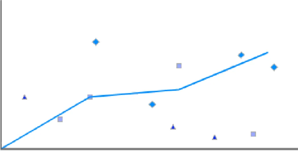
The creation of the static model is done by creating a set of points with known distances and angles that represent both valid data points, signal multipath errors and undefined outliers. A section of the static model is shown in Figure 24. The qualities of the static model are crucial for the algorithm to identify signal multipath errors, because it functions as the ground truth of signal multipath errors in the training process of the classifier.

Important for the model is to contain at least all possible types of outliers that the classifier must be able to recognize, whereby the relative distance between points must be of

(44)

the point distances for the classifier.

Another important aspect of the model is the occurrence of valid data in the model. Only supplying invalid data in the model would create overfitting effects, since the model would not be aware of the features and characteristics between valid data. The relationship between the valid and invalid data points are kept in a proportion of about 1:20to keep a realistic

relationship between the valid and invalid points.

Figure 24: Static Model

After the creation of the static model, the features of the dataset are extracted. The features contained in the dataset are the distance between the points and the angle between points. These aspects describe the underlying relation between points and provide the information needed to distinguish signal multipath errors.

The feature of a point is described by the distance in respect of the upcoming point and the angle in respect of its previous and next point as described in Figure 25.

Feature Set Data Point: {Angle, Distance, Class}

Figure 25: Direction and Distance Features of a Point

(45)

The created classifier will be tailor made for the provided dataset and will classify every point based on its features and the established class rules to be either a valid point or a signal multipath error point. Every point is assigned a specific class based on the classification rules established and will contain their feature information together with their class information.

When the data is classified, the encountered signal multipath errors must be corrected

according to the information given per error segment. The described error types as described in the Description Case Study section have different correction implementations. The classical and unrelated signal multipath errors will be corrected according to their offset created by the reflection, whereby the undefined signal multipath errors are corrected using a Kalman Filter (Welch, 1995).

This describes the solution provided by the framework. The following section will cover the actual system architecture and its design motives. The implementation of the system can vary per programming language and environment. This solution is based on an object oriented based design and is implemented using Java as its programming language.

5.5 Implementation

The described system flow describes the process needed to recognize, classify and correct errors in GPS data. Aside from these core requirements, several other functional and quality requirements are established as described in Table 1.

These requirements describe a system that allows the user to easily import, process and review

GPS datasets. Aside from the user’s perspective of the application, the developers and business perspective of the application is considered, which requires high modularity and maintainability of the system.

To facilitate these requirements, the Model-View-Controller pattern in combination with the Observable pattern is used as main components of the system architecture. Also, a layered designed is used, which separates the different functionalities of the system to strengthen the separation of concerns and reduce cross cutting concerns throughout the system.

The Model-View-Controller pattern is chosen, because the system requires an interface for the user and a logical section that describes the model of the system. Since the architecture will be used for various other applications that will require different interfaces, the decoupling of the

system’s model and interface is necessary. This separation can be well modelled using a Model-View-Controller pattern by using an intermediate Controller instance that serves as the

interface for the Model and the View. By doing so the View and the Model both only need to be aware of the interface of the controller and can be adapted and changed without knowledge of the other components of the system.

Context Aware GPS Error Correction

MASTER THESIS