Fuzzy control and its application to a pH process

University of Warwick institutional repository: http://go.warwick.ac.uk/wrap A Thesis Submitted for the Degree of PhD at the University of Warwick

http://go.warwick.ac.uk/wrap/3657

This thesis is made available online and is protected by original copyright. Please scroll down to view the document itself.

Fuzzy Control and its Application

to a

pH

Process

K. E. Huang

A Thesis Submitted to the University of Warwick for the degree of

Doctor of Philosophy

Department of Engineering

University of Warwick

Summary

In the chemical industry, the control of pH is a well-known problem that presents difficulties due to the large variations in its process dynamics and the static nonlinearity between pH and concentration. pH control requires the application of advanced control techniques such as linear or nonlinear adaptive control methods. Unfortunately, adaptive controllers rely on a mathematical model of the process being controlled, the parameters being determined or modified in real time. Because of its characteristics, the pH control process is extremeIy difficult to model accurately.

Fuzzy logic, which is derived from Zadeh's theory of fuzzy sets and algorithms, provides an effective means of capturing the approximate, inexact nature of the physical world. It can be used to convert a linguistic control strategy based on expert knowledge, into an automatic control strategy to control a system in the absence of an exact mathematical model. The work described in this thesis sets out to investigate the suitability of fuzzy techniques for the control of pH within a continuous flow titration process.

Initially, a simple fuzzy development system was designed and used to produce an experimental fuzzy control program. A detailed study was then performed on the relationship between fuzzy decision table scaling factors and the control constants of a digital PI controller. Equation derived from this study were then confmned experimentally using an analogue simulation of a first order plant. As a result of this work a novel method of tuning a fuzzy controller by adjusting its scaling factors, was derived. This technique was then used for the remainder of the work described in this

thesis.

operating characteristics, but also that the fuzzy controller was much better at controlling the highly non-linear pH process, than a conventional digital PI controller. The fuzzy controller achieved a shorter settling time, produced less over-shoot, and was less affected by contamination than the digital PI controller.

One of the most important characteristics of the tunable fuzzy controller is its ability to implement a wide variety of control mechanisms simply by modifying one or two control variables. Thus the controller can be made to behave in a manner similar to that of a conventional PI controller, or with different parameter values, can imitate other forms of controller. One such mode of operation uses sliding mode control, with the fuzzy decision table main diagonal being used as the variable structure system (VSS) switching line. A theoretical explanation of this behavior, and its boundary conditions, are given within the text.

Contents

Summary

Acknowledgements

1. Introduction . . . .. 1

1.1 pH propress Model Equations and pH Control Problems . . . .. 1

1.2 Reasons for Using Fuzzy Logic in the control of pH process . . . .. 4

1.3 Description of the Contents of this Thesis . . . .. 6

2. Theory and Design a Fuzzy Logic Controller . . . .. 8

2. 1 Basic Definitions and the Fuzzy Set . . . .. 8

2.2 Structure of a Fuzzy Controller. . . .. 12

2.3 Design considerations for an FLC . . . .. 15

2.3.1 Fuzzification strategies . . . .. 16

2.3.2 Defuzzification strategies . . . .. 17

2.3.3 Data Base consideration . . . .. 20

2.3.3. 1 Discretization / normalization methods for the universes of discourse 20 2.3.3.2 The choice of the membership functions for the primary fuzzy sets 22 2.3 .3.3 The fuzzy partition of the input and output space . . . 24

2.3.4 Rule Base consideration . . . 25

2.3.4.1 Choice of the state and control variables for the fuzzy control rules 25 2.3.4.2 The derivation of fuzzy control rules. . . .. 26

2.3.4.3 The justification of fuzzy control rules . . . .. 28

2.3.4.4 The choice of the fuzzy control rule types 29 2.3.5 Decision making logic consideration '. . . .. 31

2.4 Current uses of Fuzzy Techniques and other Non-linear methods in Control of the pH Process . . . 44

2.4.2 Dynamic Modeling and Reaction Invariant Control of pH(1983) 44 2.4.3 An Experimental Study of a Class of Algorithms for Adaptive pH

Control (1985) . . . 45

2.4.4 Non-linear State Feedback Synthesis for pH Control (1986) 45 2.4.5 Non-linear Controller for a pH Process (1990) 45 2.4. 6Non-linear Control of pH Process Using the Strong Acid Equivalents (1991) . 45 2.4. 7 Fuzzy Control of pH Using Genetic Algorithms (1993) 46 2 .4. 8 Summary . . . 46

3. Implementation of a Real-Time Fuzzy Controller

3.1. 1 The Structure of a Fuzzy Control System . . . 49

3.1.2Technical Considerations When Developing a Fuzzy Control System 51 3.2 FLC Implementation methods . . . .. 52

3.2.1 Implementation Using the FKB Compilation Method 53 3.2.2 Implementation Using the FKB Interpretation Method . . . 56

3.2.3 A Comparison of Implementation Methods . . . .. 57

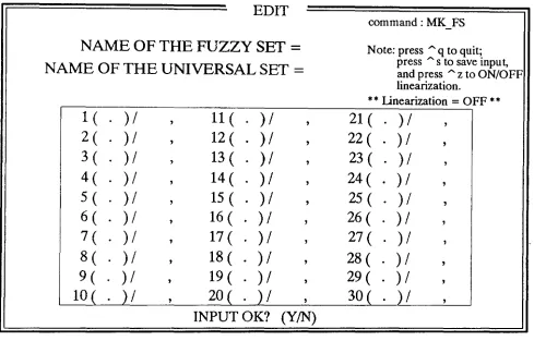
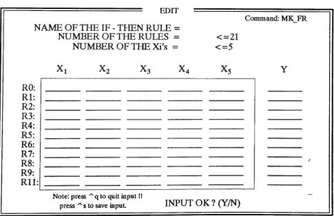
3.2.4 The Fuzzy Development System 58 3.3 Implementing an Experimental FLC . . . .. 61

3.3.1 System Description . . . .. 61

3.3.2 Fuzzy Control Program Design . . . 73

3.4 Experimental Setup for the Fuzzy Controller. . . .. 76

4. The Relationship between Fuzzy Decision Table Scaling Factors and

the Control Constants of a Digital PI Controller . . . .

4.1. Comparing Various Control Decision Tables 79 4.1. 1 A comparision of digital PI and fuzzy controllers . . . .. 79

4.1. 2 Comparing various decision tables . . . 80

4.2 Comparing Fuzzy Logic with Classical Controller Design . . . .. 82

5. The Effect of Scaling Factors on a Fuzzy PI Controller . . . ..

5. 1 Experiment setup . . . .. 88

5.3 The fuzzy PI controller experiments performe . . . 91

5.3.1 The effect of varying the decision table ranges on the behaviour of a Fuzzy PI controller and its comparison with the control constant of a digital PI PI controller. . . 91

5.3.2 Limitation of the decision table ranges . . . 94

5.4 Sliding control of a fuzzy PI controller caused by choosing too small value of D or too large value of E 101 5.4.1 The negative gain caused by choosing too small value of D 101 5.4.2 Theoretical explanation of the sliding mode control caused by the introduction of a negative gain in the controller to form a variable structure system (VSS) 105 5.4.3 Mathematical existence conditions for a sliding regime lOX 111 5.4.4 The sliding regime caused by choosing too large value of E 116 5.4.5 The sliding regime for a general first order plant controllered by a fuzzy PI controller. . . .. 121

5.5 A Fuzzy integral controller. . . .. 122

5.6 Modification of the fuzzy PI controller by temporarily switching the decision table range to a new value. . . .. 125

6. The Characteristics of the pH Process Experimental Model Plant 132 6.1. pH Process Model Equations. . . .. 132

6.2. Experiment set up . . . .. 135

6.3 Static and dynamic behavior of the pH process model plant. . . .. 137

6.3.1 Dynamic characteristics 138 6.3.2 Calibration of pH sensor and actuator. . . .. 138

6.3.3 Non-linear titration characteristics. . . .. 140

6.4 Summary . . . .. 145

7. Fuzzy Control of the pH Process . . . .. 146

7.2.1 Digital and fuzzy PI control with large K, and small

K,

7.2.3 Comparing digital and fuzzy control at pH = 8. . . .. 156

7.3 The effect of the choice of U on the fuzzy pH process control response 158 7.4 An investigation of the effects of setting the error change range D to 0.0003V or less. . . .. 163

7.5 Enlarging the D range while keeping error range E constant 165 7.5.1 The relationship between the strength of the fuzzy controller output and the sweeping area of the decision table . . . .. 166

7.5.2An experimental study between D and U 167 7.6 Fuzzy control at pH = 5

9

7.7 Fuzzy PI control for different load concentrations and with load perturbations. .. 173

7.8 Conclusions from the experiment performed . . . .. 174

8. Conclusion . . . ., 177

8.1 Assessment of the Fuzzy PI Controller . . . ., 179

8.2 Recommendations for future work . . . ., 180

Reference . . . .. 181

Acknowledgement

There are many people to whom grateful thanks are due, without them this research

would not have been possible. Firstly, I would like to thank Dr. Neil Storey and Dr. Peter

Jones for their supervision and encouragement at all stages of my study at Warwick

University. They have always given me advice and support whenever I needed it. I would

also like to thank Dr. J. F. Craine for his advice and technical support in constructing my

fuzzy control program generator.

I would like to acknowledge the support of Kuang-chih Huang, President of the

National Kaohsiung Institute of Technology in the early stages of my application for paid

leave for one year and for his encouragement during my period of study.

Special thanks go to Dr. T. I. Kuo who helped me to build my pH process control

model plant, and to Dr. M. R. Cheng who has inspired me and helped me in many ways.

Above all, my deepest appreciation goes to my family. Without their complete support

and the love of my two lovely daughters and my wife, my study in England for a doctoral

degree would not have been possible.

Chapter 1

Introduction

In the chemical industry and in waste water treatment, the control of pH (the

concentration of hydrogen ions) is a well-known problem that presents difficulties due

to large variations in process dynamics and the static nonlinearity between pH and

concentration. Usually it requires the application of advanced control techniques such

as linear adaptive control[1 ,2,3 ,4,5], nonlinear adaptive control[6] or nonlinear control

using a nonlinear transformation method[7]. However, these design methods are often

complicated, as will be seen later in the survey section of this thesis (section 2.4).

1.1. pH Process Model Equations and pH Control Problems

pH is a measure of [H+], which denotes the concentration of hydrogen ions, in a

solution. It is defmed by:

pH = -log [H+ ] (1-1)

A well established method for modeling the dynamics of pH in a stirred tank is that

developed by McAvoy[8]. This method, for single acid/single base systems, uses

F

C

~ - - Controller

Figure 1-1 pH control system.

equilibrium equations and an electroneutrality restraint. For a typical pH control system

as shown in Figure 1-1, there is a strong acid, HA, neutralized by a strong base, BOH,

with the assumptions of constant volume, perfect mixing, and no species other than

water present, the mole balances of the cation of the acid and the anion of the base are:

(1-2)

(1-3)

here, CArepresents acid anion concentration and CBrepresents base cation concentration

in _{the effluent stream. CAcid is the acid concentration in the acidic stream entering into}

this continuous stirred tank reactor (CSTR). CBase is the base concentration in the basic

stream entering CSTR. V is the volume of CSTR. FA and FBare flow rate of acidic and

basic streams. These dynamic equations will be discussed in detail in chapter 6. To

illustrate the difficulty of pH control, let

x

pH= f(x) x]

2

The graph of the function

f

in Fig 1-2. There is considerable variation in the slope of titration curves. In Figure 1-2,

it also shows the titration curve for a weak acid and strong base. It can be seen that in

this case the curve is not symmetrical about pH

=

0.02 0.015

0.01

c;ase(N) 0.005

-I~

O.OlNHAc

L---J

---~NHCl

_~

2

o

4 8

6 10 12

pH

Figure 1-2 typical titration curves. (reproduced from[9])

Since the titration curve varies drastically with pH, if the pH process has been

controlled by a conventional PI controller, the critical gain will vary accordingly. Some

values are listed below for different values of the pH of the mixture[lO].

pH Critical gain

7 0.009

8 0.046

9 0.46

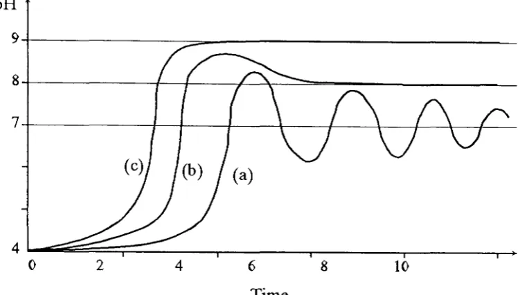
From these estimated critical gains, it showed that to make sure that the closed loop system is stable for small perturbations around an equilibrium of pH = 7, the gain should thus be less than 0.009. A reasonable value of the gain for operation at pH = 8 is k = 0.01, but this gain will give an unstable system at pH = 7 and is too low for a reasonable response at pH =9. Figure 1-3 shows a PI control with gain 0.01 to control the pH process at different set-points.

pH

9-r---:::;:~---10 8

6 4

2

7-t---t--+---+---+---f---\---,f---\--/--

8-t---f--I----I-~\__.::::=:.~---Time

Figure 1-3. The pH outputs of a pH control process which controlled by a PI controller with

set-point equal to (a)7; (b)8; (c)9.

1.2. Reasons for Using Fuzzy Logic in the Control of pH Process

Difficulties arise in the control of the pH process due to the severe process non-linearity and frequent load changes. For example, changes in the influent composition or flow rate. The non-linearity can be understood from the S-shaped titration curve shown in Figure 1-2. Frequent and rapid load changes are common for most waste water treatment facilities since the influents come from the waste of a number of sources. It

is therefore very difficult to analyze and derive the system model of a pH control process. However, experience shows that they are often controlled successfully by experienced human operator. Therefore, an alternative approach to the control of pH process is to investigate the control strategies employed by the human operators. A human operator can control a complex process effectively by simply attributing the difficulties he experienced to the rate or manner of information displayed or to the depth to which he may evaluate decisions. The operator's control strategy is based on intuition and experience, and can be considered as a set of heuristic decision rules. Usually these rules are expressed linguistically, and are often very difficult to convert into a quantitative control strategy.

The theory of fuzzy sets and algorithms developed by Zadeh[ll, 12] can be used to evaluated these imprecise linguistic statements directly. Fuzzy logic provides an effective means of capturing the approximate, inexact nature of the physical world. Therefore, it can be used to provide an algorithm which can convert a linguistic control strategy based on expert knowledge, into an automatic control strategy. The pioneering research of Mamdani and his colleagues on fuzzy control was started early in 1974 [13,14,15]. They developed a fuzzy controller for a boiler and steam engine. This showed that the fuzzy control system was less sensitive than conventional control systems to process parameter changes and that it gave good control at all operating points.

techniques for the control of pH within a continuous flow titration process.

1.3 Description of the Contents of this Thesis

The second chapter describes the basic concepts of fuzzy sets theory, fuzzy logic and

approximate reasoning and also the design considerations for a fuzzy logic controller

(FLC). Thi s material will become the basis for later chapters. At the end of this

chapter, current uses of fuzzy techniques and other non-linear methods in pH control are

discussed briefly.

FLC industrial application techniques and FLC implementation methods are

mentioned in the third chapter. After studying these implementation methods, a simple

fuzzy developing system was designed and by which an experimental fuzzy control

program was generated.

The fourth chapter gives a detailed study on the relationship between fuzzy decision

table scaling factors and the control constants of a digital PI controller. Equations

derived in this chapter are confirmed by experiments in the next chapter and become the

basic tuning tools for all the fuzzy controllers used in later experiments.

Using an analog simulation of a plant, a fuzzy PI controller was compared with a

conventional digital PI controller and described in beginning of the fifth chapter. It then

describes a detailed study of the effects of the choice of scaling factors on the control

actions of a fuzzy PI controller. It shows that, in some cases, a special sliding motion

phenomenon will happen if the error change range of the decision table is too small.

The boundary conditions of this sliding regime is also discussed. At the end of this

chapter, by using these scaling factors, several other controllers are constructed which

includes an integral controller and variable structure systems (VSS) formed by switching

A discussion of the characteristics of the pH process and its experimental models

provide the content of the sixth chapter. This includes the structure of the pH process

model plant, the m del equations and static and dynamic behavior of the process.

Chapter seven contains the results and details of the pH control experiments

performed. It shows that the fuzzy PI controller can make the system settle down easier

and faster than the digital PI controller. The damping effect caused by the decision table

near the set-point is also study in detail. Finally, the fuzzy PI control of pH process

under varying set-points and noise are tested.

The last chapter provides the conclusions drawn from this study and some

zxm ,.

Chapter 2

Theory and Design of a Fuzzy Logic

Controller

After Mamdani's work on using a fuzzy controller to control an industrial process,

reports of the application of fuzzy control techniques were widely spread through a

number of fields, such as water quality control [16], automatic train operation systems

[17], elevator control [18], nuclear reactor control [19], and roll and moment control for

a flexible wing aircraft [20]. The literature on fuzzy control has grown rapidly, and in

1990 Lee[21] produced a comprehensive survey of control applications.

The following sections give a brief description of the basic concepts of fuzzy set

theory and fuzzy logic, and includes elements from Lee's survey. This material will

form a basis for later chapters.

2.1 Basic DefInitions and the Fuzzy Set

A set U, denoted generally by {u}, is normally defined as a collection of elements

or objects that can be discrete or continuous. U is called the universe of discourse and

u are generic elements of U. Each element can either belong to or not belong to, a set

A, A E U. By defining a membership function for a set in which 1 indicates

membership and 0 indicates nonmembership, a classical set can be represented by a set

have values between 0 and 1 to represent different degree of membership for the elements of a given set. Therefore, a fuzzy set F in a universe of discourse U is characterized by a membership function I-tP, which takes values in the interval [0,1] namely,

Definition 1: Fuzzy set: A fuzzy set F in a universe of discourse U can be represented as a set of ordered pairs of a generic element u and its grade of membership function: F

= {

I

n

F =

L

1=1

where the symbol "/" is a separator and "E" means union. When U is continuous, a fuzzy set F can be written concisely as

Definition 2: Support and Fuzzy Singleton: The support of a fuzzy set F, S(F), is the crisp set of all u E U such that I-tp(u)

>

=

A fuzzy set is denoted in terms of its membership function. Therefore, the set theoretic operations of union, intersection and complement for fuzzy sets will be defined via their membership functions. Let A and B be two fuzzy sets in U with membership functions I-tA and JJ-B' respectively. Some basic operations for fuzzy sets are

Definition 3: Intersection: The membership function /lc(u) of the intersection C=AnB is pointwise defined by

U E U

Definition 4: Union: The membership function /lc(u) of the union C=AUB IS

pointwise defined by

U E U

Definition 5: Complement: The membership function Jlii.. of the complement of a fuzzy set A is pointwise defined as

P"A ( u) = 1 - PA ( u)

Definition 6: Cartesian Product: _{If AI' ... ,An are fuzzy sets in UI,'" ,Un' respectively.} Then, the Cartesian product of AI' ... ,An is a fuzzy set in the product space U IX- XUn with the membership function

P A x · · · XA (u_{1 ,} u_{2 , '} • " un) = min { PA (u_{1 ) , '} • "P A (Un)}

1 n 1 n

or

P_A x . . . xA ( _{U 1'} U2,' . . , Un) = PAl ( _{U 1 ) •} PA

2 ( U2) • . • PA ( Un)

l ' , n n

Definition 7:

Fuzzy

Definition 8: Fuzzy relation: Sup-Star Composition: If Rand S are fuzzy relations in UXV and VXW, respectively. Then the composition of Rand S is a fuzzy relation

denoted by R 0 S and is defined by

RoS = {[ (u, w), SUP(11_{R (} u, v)

*

V

Definition 9: Fuzzy number: A fuzzy number F is a fuzzy set in the continuous universe U which is normal and convex, that is

max 11_{F (} u) = 1

UEU

11_F(AU1 + (1-A)u_{2 )}

> min ( 11F( u_{1 )} ,11F( u_{2 ) ) ,}

(normal)

( convex) u_{1 '} u₂E U, A E [ 0 , 1 ]

Definition 10: Linguistic Variables: A linguistic variable is defmed by a quintuple (x,T(x),U,G,M) in which x is the name of a fuzzy variable; T(x) is the set of names of linguistic values of x with each value represented by a fuzzy number defined in U; G is a syntactic rule to generate the names for x; and M is a semantic rule to give the meaning of the x value. Usually, a linguistic variable can be regarded either as a variable whose value is a fuzzy number or as a variable whose value are defined in linguistic terms. For example, if there is a linguistic variable called "speed", then the term set T(speed) could be defined as

Each term in T(speed) is characterized by a fuzzy set in the universe of discourse U =

[0,60] as shown in Figure 2-1. where "slow" could be interpreted as "a speed below

about 15 mph", "medium" as "a speed close to 30 mph", and "fast" as "a speed more

than 45 mph", etc.

Slow Medium Fast

o ' - - - - .L..-- ~ ~ _____.J

60 45

15

o 30

Speed

Figure 2-1. Diagrammatic representation of fuzzy "speed."

Definition 11: Sup-star Composition Rule of Inference: If R is a fuzzy relation in UXV,

and u is a fuzzy set in U, then this rule asserts that the fuzzy set v in V induced by u

is given by

v =u 0 R

where u 0 R is the sup-star composition of u and R.

This defInition will become Zadeh's composition rule of inference if the star

represents the minimum operator.

2.2 Structure of a Fuzzy Controller

The basic configuration of a Fuzzylogic controller (FLC) has been described by Lee

in the survey paper discussed earlier[21]. He points out that usually there are four

principal components in a FLC as shown in Figure 2-2. These components are a

fuzzification interface, an inference engine (or decision-making logic), a knowledge base

Fuzzification interface I I I I I I I I I I I

L...- ....J tenus

FLC

1

System Actual control Nonfuzzy

Figure 2-2. Basic configuration of a fuzzy logic controller (FLC).

(1) The fuzzification interface performs the following functions:

(a) it measures the values of the input variables (or the system state variables);

(b) it transfers the range of the values of the input variables into the corresponding universe of discourse by scale mapping. Usually this is done by normalization. (c) it converts the input data into proper linguistic values which will be viewed as

labels of fuzzy set.

(2) The knowledge base consists of a database and a linguistic control rule base. Its main functions are:

(a) to provide the necessary definitions, which are used to define the linguistic control rules and fuzzy data manipulation information.

(b) to provide the control goals and control policy of the domain experts which are written using a set of linguistic control rules.

(3) The inference engine is the kernel of the fuzzy logic controller.

by fuzzy implication and the rules of inference of fuzzy logic.

(4) The defuzzification interface performs the following functions:

(a) it converts the range of values of output variables into the corresponding

universe of discourse.

(b) it generates non-fuzzy control actions from the inferred fuzzy control action

outputs.

A fuzzy system is characterized by a set of linguistic statements based on expert

knowledge, which is usually in the form of "if-then" rules of the form:

IF (a set of conditions are satisfied)

THEN (a set of consequences will be inferred).

where both the set of conditions and the set of consequences are fuzzy terms. They are

directly associated with fuzzy concepts and are referred to as "fuzzy conditional

statements". Therefore, a fuzzy control rule is a fuzzy conditional statement in which

the antecedent is a condition in its application domain and the consequent is a control

action for the system under control.

The collection of these fuzzy control rules forms the rule base or the rule set of an

fuzzy logic controller (FLC). For instance, if

x,

target plant, and y is the output of the FLC, then the IF (antecedent)-THEN

(consequence) control rule might be expressed as a control algorithms of the form:

if

x,

The antecedent (A and B) is interpreted as a fuzzy set Ax Bin the production space U xV with membership functions JLAXB(U,v) and will be discussed latter in section 2.3.5(2). Therefore, a fuzzy control rule, such as "if (x is Aj and y is Bj) then (z is Cj"

can be implemented by a fuzzy implication (relation) R, as follows:

11R ~ 11(A . /\ B .-+C .) ( u, v, w )

i J. J. J.

Where Ai and B, are fuzzy sets, AjXBjin UXV.The fuzzy implication RjA(Aj and B)

~ C, is in U xV xW; "~" denotes a fuzzy implication (relation) function which will also be discussed later in section 2.3.5(1)

2.3 Design considerations for an FLC

As mentioned earlier, the main function of the FLC is to provide an algorithm which can convert the linguistic control strategy based on expert knowledge into an automatic control strategy. Then, the principle design considerations for an FLC may be divided into five parts:

These are:

(1) fuzzification strategies; (2) defuzzification strategies; (3) data base considerations:

(a) discretization/normalization methods for the universes of discourse, (b) the choice of the membership functions for the primary sets,

(4) rule base considerations:

(a) the choice of the state and control variables for the fuzzy control rules, (b) the derivation of fuzzy control rules,

(c) the justification of fuzzy control rules, (d) the choice of fuzzy control rule types. (5) decision making logic considerations:

(a) the definition of fuzzy implications,

(b) the interpretation of sentence connectives "and" and "also", (c) the definition of compositional operators,

(d) the inference mechanisms;

These five parts will be discussed in the following sections.

2.3. 1 Fuzzification strategies

Fuzzification couldbe defmed as a mapping from an observed input space tofuzzy sets in a certain input universe of discourse. The data manipulation in an FLC is based on the fuzzy set theory, however, in control applications the observed data are usually crisp values. Therefore, fuzzification is necessary at an early stage. Fuzzification is normally achieved in one of two ways. Its results are shown in Figure 2-3(a) and (b). Both cases show an ordinary fuzzy set B intersecting with a fuzzy set A. A is a fuzzy set coming from the input signal Xc after fuzzification. In Figure 2-3(a), A is a singleton but in (b) A is a triangular fuzzy set. The two fuzzification methods are

is that no processing is required for fuzzification in this case. This strategy has been

widely used in fuzzy control applications, since it is very easy to implement.

jlA 1 - - - + - - - 1

B

X

o (a) Fuzzy singleton A.

Jl

(b) Triangular fuzzy set A

a

Figure 2-3.methods of fuzzification: The measured data are (a) converted to a fuzzy singleton. (b) converted to a triangular fuzzy set.

(2) In many applications the observed data are disturbed by random noise. In this

case, it is more appropriate to choose an isosceles triangle as the fuzzification function.

The vertex of this triangle corresponds to the mean value of a data set, while the base

is twice the standard deviation of the data set. Then, we can use this fuzzy number for

control manipulation. Figure 2-3(b) shows the second method of fuzzification. The fuzzy

set A with its vertex at Xo and having the base width equals to 20- is the resulting

triangular set. The point Xo is the mean value and 0- is the standard deviation of the

measured data set.

2.3.2 Defuzzification strategies

In many practical applications a crisp control action is required to drive the system.

represents the possibility distribution of the inferred fuzzy control action. In other words,

the defuzzification process is a mapping between a space of fuzzy control actions

defined over an output universe of discourse, and a space of non-fuzzy control actions.

There are several kinds of strategies being commonly used. These include the maximum

criteria, the mean of maximum and the center of area methods.

(a) The maximum criteria method

This method produces the point at which the possibility distribution of the control

action reaches a maximum value.

(b) The Mean of Maximum Method (MOM)

The MOM strategy generates a control action which represents the mean value of all

local control actions whose membership functions reach the maximum. In the case of

a discrete universe, the control action will be expressed as

n

Zo =

L

j=l

where w_j is the support value at which the membership function value p-/wj ) reaches the

maximum, and n is the total number of such support values.

(c) The Center of Area Method

The COA method is the most popular method currently being used by control

engineers. This strategy generates the center of gravity of the possibility distribution of

In the case of a discrete universe, the method yields

(d) The Center of Sums

This method is the same as the CGA method except that the overlapping areas of the

membership functions must be counted twice during the calculation. The calculation

formula is adjusted as

f zz·fJ.1c( z) dz

fzf

(e) The Height method

This method issimpler than the CGA approach, since there is no integration during

calculation. The calculation formula is

v:«.».

Zo =

where hi is the strength of the inferred antecedent output of the ith rule, and

z,

Braae and Rutherford[22] have performed detailed analysis of various defuzzification

those obtained with a conventional PI controller. However, the MOM strategy yields a better transient performance, while the COA method is better in its steady state performance.

2.3.3 Data Base consideration

The concepts associated with a data base are used to characterize fuzzy control rules and fuzzy data manipulation in an FLC. Since these concepts are basically defined according to experience and engineering judgement, a "good" choice of the membership functions of a fuzzy set will play an essential role in the success of the fuzzy controller application. In this section some of the important considerations relating to the construction of the data base will be discussed.

2.3.3. 1Discretization / normalization methods for the universes of discourse

The method used for the representation of linguistically described information using fuzzy sets usually depends on the nature of the universe of discourse. A universe of discourse in a FLC may be either discrete or continuous. If it is continuous then some discretization and normalization process will be needed before the primary fuzzy sets are applied on it.

(a) Discretization: The process of discretizing a universe of discourse is frequently referred to as the quantitization process. This process divides a universe of discourse into a number of segments.

Table 2-1

Quantization and Primary Fuzzy sets Using a Numerical Definition

Level No. Range NB NM NS ZE PS PM PB

-4 x <-4 1 0.7 0 0 0 0 0

-3 -4<x~-2.5 0.7 1 0.5 0 0 0 0

-2 _{-2.5 <x<-1.5} 0 0.7 0.7 0 0 0 0

-1 -1.5 < x< -0.5 0 0.3 1 0.3 0 0 0

0 -O.5<x<O.5 0 0 0.3 1 0.3 0 0

1 O.5<x<1.5 0 0 0 0.3 1 0.3 0

2 1.5<x~2.5 0 0 0 0 0.7 0.7 0

3 2.5<x<4 0 0 0 0 0.5 1 0.7

4 4<x 0 0 0 0 0 0.7 1

levels with 7 primary fuzzy sets defined on it. Note that the scale mapping of the measured variable values x into the discretized universe can be uniform or nonuniform. Looking into Table 2-1 we fmd that it is not a uniform mapping, since the width of the ranges for all the quantitization levels are equal to 1 except level 3. The shape of the membership functions of primary fuzzy sets, such as ZE and PM, will be discussed in

next section.

(b) Normalization: The normalization of a continuous universe requires a discretization of the universe of discourse into a finite number of segments, with each segment mapped into a segment of the normalized universe. Then, using an explicit function, a

I

fuzzy set will be defmed to its membership function. One example is shown in Table 2-2. where the universe of discourse, [-6, +4.5] is mapped into the normalized interval

Table 2-2

Quantization and Primary Fuzzy sets Using a Numerical Definition

Normalized Normalized Primary Fuzzy

Universe Segments Range _f.1 a Sets

[-1.0,-0.5] [-6.9,-4.1] -1.0 0.4 NB

[-0.5,-0.3] [-4.1,-2.2] -0.5 0.2 NM

[-0.3,-0.0] [-2.2,-0.0] -0.2 0.2 NS

[-1.0,+ 1.0] [+0.0, +0.2] [+0.0, + 1.0] 0.0 0.2 ZE

[+0.2, +0.6] [+ 1.0,+ 2.5] 0.2 0.2 PS

[+0.6, + 1.0] [+2.5,+4.5] 0.5 0.2 PM

1.0 0.4 PB

2.3.3.2The choice of the membership functions for the primary fuzzy sets

There are two kinds of fuzzy set definitions, depending on whether the universe of

discourse is discrete or continuous.

(a) Numerical Defmition: In this case, the grade of membership function of a fuzzy set is represented by a vector of numbers. The dimension of the vector depends on the degree of discretization. If the membership function of a primary fuzzy set of this kind

has the fonn

7

=

L

a

. 1 u .

.1.= ~

where a

=

u,

o

ZE

= [ - , - ,

-4 -3

o

- ,

-2

0.3 -1 '

1

-,

_o

Therefore, under this definition a fuzzy singleton will have the form of s= [0,0,0,0,0, 1,0] without showing its value of quentitization level.

(b) Functional Definition: The membership function of a fuzzy set can sometimes be expressed in a functional form, typically using triangle or bell shaped functions. It is very easy to describe a triangle shape by function, for example, one could define a triangle fuzzy set named "slow", which has vertex at 20 km and two base points at

°

and 40 lan. The following function can then be used to calculate its grade:

].1slow(x) = 20 -

Ix -

l

20 , i f 0~x~40

When using bell shaped fuzzy sets, a Gaussian normal distribution curve is commonly used. This may be described by the equation:

f( x )

=

202

where Jl denotes the mean value and (J denotes the standard deviation.

The method used to assign the grades of membership to the primary fuzzy set using these functions is very important. If the incoming signals are disturbed by noise, then the membership functions should be wide enough to reduce the sensitivity to this noise. Methods of storing these functional fuzzy sets within computer memory will be discussed later. Figure 2-4 and 2-5 shows the triangle and the Gaussian curve shaped

o

1

I1(X)==a-(a-\x-b\)VO,

a>O

1 NB NM NS

zo

Figure 2-4. The triangle shaped fuzzy sets.

1 NB NM NS

zo

1

o

o

-1

Figure 2-5. The bell shaped fuzzy sets

2.3.3.3The fuzzy partition of the input and output space

Within fuzzy systems, both the input (antecedent) and output (consequence)

linguistic variables form fuzzy spaces with respect to their own universes of discourse.

In general, a linguistic variable is associated with a term set, with each term in the term

set being defmed on the same universe of discourse. A fuzzy partition determines how

many terms exist within the term set. A fme partition produces more terms than a coarse

one. Figure 2-6 shows two typical examples of fuzzy partitions in the same normalized

universe [-1,

+

1

o (b) partition of the fuzzy input!output

control rules is 7x7 =49.The fuzzy determines the maximum number

of fuzzy control rules that can be

coarse

1 N Z P

constructed. For instance, in the case of two-input, one-output fuzzy

0

controller, if the cardinalities of the -1 _(a)0 1

term sets of these two inputs are all

finer

1 NB NM NS ZE PS

7, then, the maximum number of

space, is normally non-deterministic and has no unique solution. A

Figure 2-6. Diagrammatic representation of fuzzy partition. (a) 3 terms coarse partition(b) 7 terms finer partition. heuristic cut and trial procedure is

usually needed to get the appropriate number of fuzzy partitions.

2.3.4 Rule Base consideration

A primary task in the design of a fuzzy controller is the construction of the control rule base. Topics to be considered include: the choice of process state and control (output) variables; the derivation and justification of control rules; the type of fuzzy control rules to be used; and issues of consistency, interactivity, and completeness [21]

of control rules.

2.3.4.1 The choice of the state and control variables for the fuzzy control rules

state error integral, the state error derivative, etc.

2.3.4.2The derivation of fuzzy control rules

Tagaki and Sugeno [23] concluded that there are four ways to generate a set of fuzzy control rules. These four ways are not mutually exclusive, and may be combined to form an effective way to construct the fuzzy control rules.

(a) Using Expert Experience and Control Engineering Knowledge:

In everyday live most of the information on which our decisions are based is linguistic rather than numerical in nature. In this respect, fuzzy control rules provide a natural framework for the characterization of human behavior and for analyzing the decision making process. It was realized that fuzzy control rules could provide a convenient way to express domain knowledge. Therefore, most FLCs are based on the knowledge and experience which are expressed in the language of fuzzy if-then rules [14],[24] ,[25].

The formulation of fuzzy control rules can be done in two ways. The first one involves an introspective verbalization of human expertise. Examples of such verbalization are those operating manuals for the production plant. The second includes an interrogation of experienced experts or operators using a carefully organized questionnaire. By these two methods a prototype set of fuzzy control rules can be produced for a particular application. However, it will generally be necessary to optimize the performance of the system using a trial and error approach.

(b) Using lnfonnation on Operator's Control Actions:

not known sufficiently clearly, to make it possible to employ classical control theory for

modeling and simulation. However, human operation can perform quite complex tasks

in the absence of such models. For example, a skilled driver can park a car successfully

without being aware of a quantitative model of the car. In fact, a set of fuzzy if-then

control rules is being employed consciously or subconsciously by the car operator.

Therefore, rules deduced from the observation of a human controller's actions, are a

useful source of information of a rule base. Sugeno has presented a series of papers

discussing the automation of this process [26][27][28].

(c) Using a Fuzzy Model of a Process:

By analogy with classical control system modeling, a linguistic description of the

dynamic characteristics of a control system can be viewed as a fuzzy model of the

system. Based on this fuzzy model, it is possible to obtain a set of fuzzy control rules

for achieving near optimal control of the system. This set of control rules can then be

used as the rule base of an FLC.

Some fuzzy modeling techniques have been reported [29] [30], but this approach to the design of an FLC has not been fully developed [21].

(d) Using Technique Based on Learning:

Early in 1979 Procyk and Mamdani presented the first self-organizing controller

(SOC)[31]. Such controllers are very attractive in applications as they automatically

tune, and retune, themselfs on line, and require no special expertise from the operator

once installed [45] . The SOC has a hierarchical structure which consists of two rule

bases. The first is the general fuzzy rule base of an FLC. However, the second is

base, based on the desired overall performance of the system. In 1991, Lee presented a new method of SOC [32]. He employed an approximation reasoning and neural net concept for a self-learning rule-based controller. In Lee's controller there are two very important units: the Associative Critic Neuron (ANC), and the Associative Learning Neuron (ALN). The former evaluates the output response produced by present control action and creates an evaluation signal. The latter adjusts the break point of the membership functions in the rule base based on signals received from the ACN. Combining neural network theory with fuzzy control theory is seen as an area of great potential in the design of FLCs.

2.3.4.3The justification of fuzzy control rules

The most common method applied to the justification of fuzzy control rules is called "scale mapping", which was first presented by King and Mamdani [33]. Rule justification is done by considering the nature of the response of the system when plotted on a phase plane diagram. This process is best understood through the use of an example phase plane analysis.

Consider a system using the error E and change of error DE as input variables and a rule linguistically described as follows:

IF E (error) =PB and DE (change of error) =PS THEN y (output) =NM

( PB: positive big, PS: positive small, NM: negative medium.)

changed to NB. This would increase the retarding force to reduce the overshoot or

adjust the value of membership function for NM to improve it.

A similar method was suggested by Braae and Rutherford [34]. They tracked the

linguistic trajectory of the closed loop system in a 'linguistic phase plane' . The pmciples

involved in this approach is similar to those described above.

DE

c

/

over shoot

E

rise time

s.p,

a

E +

DE

m

+ + - - + + - - + + time

+ + - - + + + +

-(a) phase plane trajectory (b) system step response

Figure 2-7. Rule justification by using phase plane.

2.3.4.4 The choice of the fuzzy control rule types

Two types of fuzzy control rules are currently in use in the design of FLCs. These

are "state evaluation" fuzzy control rules and "object evaluation" fuzzy control rules. A

third type, slightly modified from the first of these, is also quite popular in the industrial

application. Its consequent instead of using linguistic values is represention as a function

of the process variables. These three types of fuzzy control rules are discussed briefly

below

(a) State Evaluation Fuzzy Control Rules:

State evaluation fuzzy control rules are the most commonly used form of rules in

characterized by the following form

where X,'" ,yand z are linguistic variables representing the process state variables and

the fuzzy control output variable; Ai,"',Bj and C, are the linguistic values of the

linguistic variables x, "',y, and z.

(b) State Evaluation Fuzzy control Rules with Functional Output :

In such rules, the consequent is represented as a function of the process state

variables X,"',y .i.e.,

R: if

x

hex, ...

Such type of rules were first proposed by Sugeno[23], and are now widely used in

industry.

(c) Object Evaluation Fuzzy Control Rules:

Fuzzycontrol using objective evaluationcontrol rules is also called 'predictivefuzzy

control', and was first proposed by Yasunobu, Miyamoto, and Ihara[35]. A control

command is inferred from an objective evaluation of a fuzzy control result that satisfies

the desired states and objectives. The rule will be described as

A control command u takes a crisp set as a value, such as "changed" or "not changed", and x, y are performance indices for the evaluation of the ith rule, taking values such as "good" or "bad". Then the most likely control rules will be selected through predicting the results (x,y) corresponding to every control command C,

This rule can be interpreted linguistically as: "if the performance index x is A_j and index y is Bj when a control command u is chosen to be C, then this rule is selected

and the control command C, will be taken to be the output of the controller. "

In practical, it is possible that more than one system state will give the same result and prediction becomes more complicated.

2.3.5 Decision making logic consideration

The use of an FLC can be viewed as trying to emulate human decision making within the conceptual framework of fuzzy logic and approximate reasoning. In this context, the forward data-driven inference (generalized modus ponens), this term will be explained later, plays a very important role. In this section, the properties of fuzzy implication functions, sentences connectives, composition operators and related concepts will be introduced.

(1) Fuzzy Implication Functions

A fuzzy control rule, is essentially a fuzzy relation which is expressed as a fuzzy implication. In fuzzy logic, a fuzzy implication may be defmed using some kind of

fuzzy implication functions.

(a) Basic properties of a fuzzy implication function:

generalized modus tollens (GMT), both of them come from tautologies such that modus

ponens: (A1\(A~B))~B, and modus tollens: «A~B)1\(not B))~ not A. Here, "~" is

the fuzzy implication or relation usually denoted by relation matrix "R". If A, A', B,

and B' are fuzzy predicates.then these two rules can be described as following,

premise 1: x is A'

premise 2: if x is A then y is B consequence: y is B'

premise 1: y is B'

premise 2: if x is A then y is B consequence: x is A'

(GMP)

(GMT)

For the GMP case, "y is B'" results from matrix operation B' =A' 0 R.It has forward

data-driven characteristics, thus which is more suitable for ordinary control applications.

(b) Families of Fuzzy Implication Functions:

There are at least 40 different kinds of fuzzy implication functions, in which the

antecedents and consequences contain fuzzy variables. Before the inference mechanisms

are discussed, in this section, several definitions must be briefly introduced.

Definition 1: Triangular Norms: The triangular norm

*

For all x,y E [0,1]:

intersection

algebraic product

bounded product

drastic product

x A Y - min {x,y}

x . y = xy

x

0

=

x y

=

x@y= y x

=

Definition 2: Triangular Co-Norms: The triangular co-norm

+

function denoted by +:[0,1] X[O,l] ~ [0,1], which includes

union

algebraic sum

bounded sum

x V Y - max{x,y} x ~ y - x + y - xy

X $ Y

=

drastic sum

y = l

x = 1

x,y < 1

Definition 3: Fuzzy conjunction: The fuzzy conjunction is defined for all u E U and

v E V by

A~B=AXB

=

f

l/XV

where

*

Definition 4: Fuzzy disjunction: The fuzzy disjunction is defmed for all u E U and v

E Vby

A~B=AXB

=

f

l/XV

where

+

Definition 5: Fuzzy Implication: There are five families offuzzy implication functions in use. Here, as before,

*

+

a) material implication

A ~ B - (not A)+ B

A ~ B = (not A)+ (A* B)

c) Extended propositional calculus:

A ~ B

=

d) Generalization of modus ponens:

A ~ B

=

e) Generalization of modus tollens:

A ~ B

=

inf {

Based on these definitions, many fuzzy implication functions may be generated by

employing triangular norms and co-norms. Examples include the following fuzzy

implications, which are called the mini-operation rule of fuzzy implications and the

product operation rule of fuzzy implication. These were developed by Mamdani[13] and

Larsen[65] respectively, and are often used in FLCs.

mini-operation rule:

R_c = A ~ B

=AXB

=

f

{/Xv

product-operation rule:

R_p = A x B

=

f

{/Xv

(2) Interpretation of Sentence Connectives "and" and 'also"

(2-1)

(2 -2)

Commonly, the sentence connective" and" is implemented as a fuzzy conjunction in

a Cartesian product space in which variables are taking values from different universes

interpreted as a fuzzy set AXBin the product space UX V,with the membership function

given by

(2-3)

or

(2-4)

Where U and V are the universe of discourse associated with A and B respectively.

When a fuzzy system is characterized by a set of fuzzy control rules, the ordering of

the rules is immaterial. This implies that the sentence connective "also" should have the

properties of commutativity and associativity. Therefore, the operators in triangular

norms and co-norms possessing these properties are suitable to be used to interpret the

connective "also".

Finally from the practical point of view, the computational aspect of FLC require a

simplification of the fuzzy control algorithm. Therefore, Mamdani's R, and Larsen's ~ with the connective "also" as the union operator "V " seems to be more suitable for

constructing fuzzy models.

(3) Compositional operators

Four kinds of compositional operators have been reported which can be used in the

compositional rule of inference:

sup-min operation (Zadeh, [36])

sup-product operation (Kaufmann, [37])

sup-bounded-product operation (Mizumoto,[38])

sup-drastic-product operation (Mizumoto, [38])

In practical FLC applications, the sup-min and sup-product compositional operators

(4) Inference Mechanisms

In an FLC, the consequence of a rule is not applied to the antecedent of another.

This means that there is no chaining inference mechanism involved, and that the control

actions are simply based on one-level forward data-driven inference (GMP).

Combining all the implication functions, definitions and relations mentioned in this

chapter, the inference mechanism can be explained by the following four types of fuzzy

reasoning method which are currently employed in FLC application.

(a) Fuzzy Reasoning of the First Type - Mamdani's Minimum Operation Rule as a

Fuzzy Implication Function:

This type is the most popular reasoning method, and was first introduced by

Mamdani. Let us consider the following general form of MISO fuzzy control rules for

the case of two-input/ single-output fuzzy systems:

R_{I :} if Xl is All and x2 is A l 2 then y 1S BI

or

R_{2 :} if Xl 1S An and X 2 is A 22 then y 1S B2

or

· ·

· ·

· ·

• • •

is and is _{A i 2} then

.

R_{i :} if Xl Ail X 2 Y 1S

· ·

·

•

·

·

·

is and is _~2 then

.

~: if Xl ~l X 2 Y 1S

If the universe of discourse of

x,

Xl' X

2 and Y. Then, using equation (2.1) and (2.3), the i's control rule can he expressed

by a fuzzy relation matrix:

This system consists of n rules, R_{I,R2 , ...},Rnt!lerefore, we may combine them by "U"

as connective "also" which has been discussed in section 2.3.5(2). Equation (2.5)

becomes

R = R UR U ... UR

I 2 n

n

=

U

s,

i=l

( 2 .6)

When the inputs are

Aol

Ao2

or

B_O(y) = max [R( Xl' _{X 2,}y)

A

A

X I,X2

(2.7)

(2.8)

Normally, the control inputs are crisp values, which are called fuzzy singletons. In this case, we can replace the antecedent variables

x.,

Xm,

( 2 .9)

and equation (2.7) become

(2.11) combining (2.5) and (2.6), the right hand side of (2.11) will become

• • •

n,

if we define

then (2. 11) will becomes:

n

B_o(y)

=

V

i=l

(2.13)

(2.14)

(2.15)

Now, if we use the center of area method (eGA) to get the defuzzification output, then we will have a crisp output value. As described in section 2.3.2(c) the defuzzification formula is

Yo =

J

B_o(y) 'ydy

J

(2.16)

The following figure shows the reasoning method of this type.

Xz

B

-y

Xz

Xoz

y

(b) Fuzzy Reasoning of the Second Type - Larsen's Product Operation Rule as a Fuzzy Implication Function.

Fuzzy reasoning of the second type is based on the use of Larsen's product operation rule

R,

ith

(2.17)

consequently, the result of reasoning will become

n

B_o(y) =

V

(2.18)

The fuzzy reasoning process is illustrated in Fig. 2-9 as shown below

Y Y

W_z

.. ---+---:

X02

Yo

(c) Fuzzy Reasoning of the Third Type - Tsukamoto's Method with Linguistic Terms

as Monotonic Membership Functions:

This method was proposed by Tsukamoto[39]. It is a simplified method based on the

fuzzy reasoning of the first type in which the membership functions of fuzzy sets Xl'

X₂ and Y are monotonic, as shown in Figure 2-10(a) and 2-10(b).

1 1 - - -

-Positive

0

-1 0 1 -1 0 1

(a) (b)

Figure 2-10(a) monotonic linear type fuzzy membership function.

(b) monotonic arctan type membership function.

The P(Positive), N(Negative) fuzzy variables can be described as

P(x) = - x1 + 1

2 2 (2.19)

N(x) = P( -x) (2.20)

for Figure 2-10(a), the monotonic linear type variables. and

P(x) (2.21)

N(x}

Pc-x}

for Figure 2-10(b) the arctan type variables.

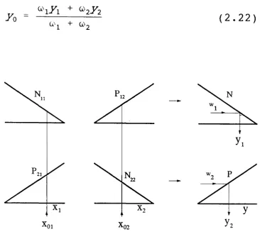
If using Tsukamoto's method, the result inferred from the first rule is Wt such that

crisp control action may be expressed by equation (2.22), the height method, which has

been described in section 2.3. 2(e). This type of fuzzy reasoning is illustrated in Figure

2-11.

(2.22)

--y

Figure 2-11. Diagrammatic representation of fuzzy reasoning type 3.

(d) Fuzzy Reasoning of the Fourth Type - The Consequence of a Rule is a Function of

Input Variables.

Fuzzy reasoning of the fourth type employs a modified version of the state

evaluation function. In this mode of reasoning, the ith fuzzy control rule is of the form

here, we may consider both f1 and f2 as linear equations of the form

although these are not usual in many applications. If the input variables are Xo1 and Xo2, then the inferred value of the first and second rules will become

Thus, applying these two values, we can calculate the consequence result directly as

Finally, using the eGA defuzzification formula, a crisp control action is given by

Yo

=

WI + _{W 2} (2.23)

of input space partitioned. Figure 2-12. shows an example of the fuzzy rules used when

two input variables are involved, and Figure 2-13 shows the corresponding partitioning

of the input space. Note that, the break points of the membership functions for the input

variable

x,

those membership function overlapping zones.

if X₂ then y

---_.

Y1 = 1.0 Xl + 0.5X₂ +1.0

Y4 = 0.2 Xl +0.lx₂ +0.2

Y3 = 0.9 x , +0.7x₂ +9.0 Y2 =-0.1 Xl + 4.0X₂ +1.2

h

3 9

/1

3 9

~L

--,,---,-L

L

4 13

Figure 2-12. The fuzzy rules for reasoning of type 4.

Deciding on an appropriate method of partitioning is a serious problem from the fuzzy

system identification point of view[40,41].

13

-1

4

-3 9 11 18

2.4 Current uses of Fuzzy Techniques and other Non-linear methods in Control of the

pH Process

As mentioned in Chapter 1, control of the pH process is difficult due to the

non-linearity and time varying nature of the titration curve, and because of its strong

sensitivity to disturbances near the point of neutrality. For these reasons, over the years

several new technologies have been applied in an attempt to solve these problems. In

this section, several different approaches, including the use of the fuzzy logic are listed

chronologically and briefly discussed.

2.4.1 The Digital Parameter Adaptive Control Technique (1980)

Bergmann& Lachmann's paper[3] published in 1980, describes the application of

two digital parameter adaptive controllers to a pH process. The controllers use

combinations of recursive least squares (RLS) parameter estimation methods with a extended minimal variance controller and a deadbeat controller of increased order. These

two adaptive control algorithms have been applied to control a pH pilot plant.

Experimental results are promising. However, selecting appropiate parameters to

achieve good stability is very difficult.

2.4.2 Dynamic Modeling and Reaction Invariant Control of pH(1983)

In 1983, Gusstafsson and Waller presented a paper[5] on a general and systematic

approach to the derivation of dynamic models for fast acid-base reactions. The treatment

is based on a consistent use of chemical reaction invariants and variants, the former

describing the physical properties of the reactor system independent of chemical

reactions, the later describing the chemical reactions. For fast acid-base reactions the

The reaction rate vector is thus eliminated from the model. The reaction variant part of

the model then, use a static equation to relate pH to the reaction invariant state

variables. The model obtained provides a sound basis for the design of control loops for

a pH control process. A computer simulation example is given at the end of this paper.

2.4.3 An Experimental Study of a Class of Algorithms for Adaptive pH Control (1985)

This paper, which was published by Gustafsson in 1985[4], describes models suited

to the design of controllers of pH in fast acid-base reaction processes with varying

buffer concentrations. The set of models includes a non-linear model resulting in a

controller with linearized feedback of a reaction invariant state vector and linearized

models resulting in adaptive linear feedback of pH. Experiments showed that the

reaction invariant feedback control needs a

priori

dynamics of the process, which includes the time delay n and the model orders n_A and

nB• These models can be obtained by on-line identification performed by a self-tuning

regulator. However, to ensure a correct result when identifying a process in closed-loop,

feedback polynomials of a high enough order and extra perturbing inputs are necessary.

In this paper the emphasis is put only on the adaptive properties of the controllers.

2.4.4 Non-linear State Feedback Synthesis for pH Control (1986)

Inthis paper, presented by Wright and Kravaris[7] , a novel non-linear state feedback design methodology is described. This is based on a non-linear transformation of the

output that linearizes the state/output map. A linear PID control law for the transformed

output generates a non-linear control law for the pH process. Computer simulations were

used to compare the performance of this non-linear control law to classical linear PID

approximately 10 controller actions, is clearly superior than the classical contro at all

sampling periods.

2.4.5 Non-linear Controller For a pH Process (1990)

Jayadeva and Rao, etal[42] synthesized a non-linear feedback-feedforward controller

in which a model reference non-linear controller design technique is applied to control

a pH process. The performance of this non-linear controller is evaluated by simulation

both for regulatory and servo problems. The simulation result is very good. This control

system is also shown to be robust to significant parameter variations and to small

disturbances.

2.4.6 Non-linear Control of pH Process Using the Strong acid Equivalents (1991)

A novel approach was developed by Wright and Kravaris[43] for the design of

nonlinear controllers for pH processes. It consists of defining an alternative equivalent

control objective which is linear in the states and using a linear nonadaptive control law

in terms of this new control objective. The new control objective is interpreted

physically as the strong acid equivalent of the system.

A minimal order realization of the full-order model has been rigorously derived, in

which the titration curve of the inlet stream appears explicitly. The strong acid

equivalent is the state in the reduced model which can be calculated on line from pH

measurements given a nominal titration curve of the process stream. However, this

requires the use of additional hardware, such as an automatic titrator or ion-selective

eletrodes to obtain a direct or indirect measurement of the strong acid equivalent value.

Computer simulations have been used to evaluate the performance of this new