On the application of extreme interaction torque with an underactuated UAV

On the Application of Extreme Interaction Torque with an

Underactuated UAV

M.J.W. (Max) Snippe

M

Sc Report

Committee:

Prof.dr.ir. S. Stramigioli

Dr.ir. J.B.C. Engelen

H. Wopereis, MSc

Dr.ir. R.G.K.M. Aarts

Dr.ir. A. Yenehun Mersha

August 2018

033RAM2018

Robotics and Mechatronics

EE-Math-CS

University of Twente

On the Application of Extreme Interaction Torque

with an Underactuated UAV

Marcus J.W. Snippe

Abstract—This paper aims at setting the initial steps towards the application of extreme interaction torque using an underac-tuated Unmanned Aerial Vehicle (UAV). Extreme torques are considered torques significantly larger than what UAVs can intrinsically generate.

An optimization algorithm is designed that uses predetermined constraints, a desired application torque, and UAV parameters to derive an optimal manipulator and input force and torques for the UAV. The optimization minimizes a nonlinearly constrained cost function and returns an optimal homogeneous transforma-tion matrix and input covector. During optimizatransforma-tion, the resulting torques and forces are scaled using a weighting function, which allows to assign priority to certain force or torque elements in the application point.

To validate the optimization, the specific use-case scenario of fastening a bolt is used. The UAV parameters and desired appli-cation torque are selected for this use-case and the optimization is executed. The weighting function is used to prioritize that undesired torques and forces remain small.

The optimal transformation is validated by means of a static simulation. A certain theoretical maximum torque is considered as reference. This is the maximum that can be reached with the determined UAV weight, maximum thrust, and effective manipulator arm length. The results indicate that the achieved desired torque reaches 67% of its theoretical maximum. The undesired torque reaches only 41% of the value it has when the theoretical maximum of the desired torque is applied. For the chosen UAV, the achieved desired torque is more than 7 times larger than what the UAV can generate intrinsically.

The applicability of the optimization for the chosen use-case is validated by a dynamic simulation with a specifically derived controller. To that end, a dynamic rigid body model of the optimized manipulator on the UAV is derived using screw theory for rigid body dynamics. A Finite State Machine (FSM) is used to solve the problem of fastening a bolt with limited allowed displacement. Fuzzy Inference System (FIS) evaluation based on an estimate of the current damping friction is used to adapt the controller to the unknown friction model of the bolt.

The results show that the chosen controller structure is capable of fastening the bolt to a desired tightening torque. The adaptive FIS PID controller effectively deals with the complex friction torque, but performance can probably be improved by reconsidering the semantic rule-set. The simulation results imply that the chosen motion profile setpoint might not be as effective as a critically damped PID controller with step reference input.

Index Terms—UAV, aerial interaction, torque application

I. INTRODUCTION

T

HE range of applications of UAVs is extensive, dueto their mobility and agility. Until shortly, UAVs were mostly used for passive tasks, such as photography/filming, passive inspection, and surveillance. Aerial interaction has increased the range of applications even more. UAV now are able to actively interact with their environment to execute tasks

as opening doors, pick-and-placing, and even building rope bridge-like structures [1]–[4].

Although aerial manipulation has been a subject of research for several years, the manner of manipulation is limited to fairly low interaction wrenches. The main reason for this is the fact that UAVs are free floating bodies, contrary to for example a stationary robotic arm with a fixed base. Therefore they are unable to close the force cycle with the environment and thus must intrinsically deliver the reaction forces, which considerably limits the maximum interaction forces and torques for UAVs.

In 2012, a lightweight and versatile manipulator was devel-oped specifically for use on a ducted-fan UAV, which allowed compliant interaction with the environment for non-destructive testing [5]. Scholten, Fumagalli, Stramigioli,et al.controlled

this manipulator while in contact based on interaction control to follow a path on a surface with the end-effector, whilst simultaneously exerting a force on the surface [6]. For the use in free-flight, a control strategy was derived subsequently that incorporates the dynamics of the manipulator and uses it to improve path tracking performance and maneuverability [7].

To counter the under-actuatedness of UAVs, McArthur, Chowdhury, and Cappelleri endowed a tricopter UAV with an reversible rotor generating thrust that works in the horizontal plane, which adds an additional actuated direction [1]. Several fully-actuated UAVs have been developed by tilting the rotor axes slightly [8]–[10].

More in the direction of applying extreme forces and torques, several control approaches for handling high energy impacts were compared and a manipulator capable of con-verting the kinetic energy to potential energy and storing it permanently was realized [11], [12]. The results of the latter where used to enable a UAV to perch on a smooth surface to stretch battery-life and consequently the possible air-time of a UAV [13].

UAVs can intrinsically generate limited torques about their

ˆ

x and yˆ axes that are mainly used for maneuverability. By

making UAVs able to execute tasks that demand significantly larger interaction torques than those that UAVs can intrinsi-cally generate, their range of applications can also include tasks like drilling holes, tightening or loosening bolts, or grinding or cleaning surfaces. To that end, this study will attempt to answer the following question:

“How can an underactuated UAV be used to apply an extreme torque on an axis perpendicular to a vertical surface?”

Where ‘extreme’ is used to indicate that the torque is

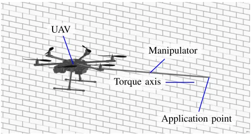
UAV

Manipulator

[image:4.612.48.301.54.189.2]

Application point Torque axis

Fig. 1. Example of a UAV endowed with a rigid manipulator that is able to use its thrust to exert a torque on the application point.

A more specific definition of these torques will be provided further on.

Firstly, the problem is elaborated and the proposed approach and used notation are described in the following section. Subsequently, an optimization of a rigid manipulator is derived in section III and a controller is designed for a specific realistic use-case in section IV. The simulated experiments will be described alongside their results in section V. Finally sections VI and VII will discuss and conclude the paper.

II. PROBLEM ANALYSIS

A. Problem description

Miniature to small scale UAVs (with a gross take-off weight up to 10 kg and an arm length of up to 0.5 m) can intrinsically generate torques in the order of 0 to ±15 N m. Therefore, these UAVs are unable to execute tasks with higher required torques, e.g. tightening a metric M10 bolt to its recommended tightening torque requires at least 30 N m, depending on its grade and material1_.

In this paper an attempt is made to derive a method to exert an extreme torque on an axis perpendicular to a vertical surface by using an underactuated UAV of miniature to small scale. A torque is considered extreme if it is at least five times as large in magnitude as the torque that the UAV can intrinsically generate about any of its principle axes. To amplify and concentrate the force and torques that the UAV can generate, the choice is made to endow the UAV with a rigid manipulator. This manipulator can be attached to the UAV either with a joint, or rigidly fixed. Figure 1 shows an example of how the UAV would be positioned with respect to the surface and the application point.

To be able to exert extreme torques using an underactuated UAV, the following points have to be taken into account.

• UAVs in single contact2cannot close the force cycle with

their environment and therefore must be able to withstand the torques that they apply to maintain an equilibrium state.

• The maximum torques and thrust of an underactuated

UAV are limited and coupled, as will be shown in

1_{https://www.blacksfasteners.co.nz/assets/Metric-8 12466 1.pdf} 2_{Contact without anchoring to another contact point.}

section III-B. The payload of a UAV is limited further by the gravitational acceleration of its own mass and the mass of the intended manipulator.

• The mass and inertia of the manipulator will also

con-tribute to the dynamics of the system. The UAV must still be able to fly in free-flight, without completely saturating its input force and torques.

• The UAV with the intended manipulator will have to be

positioned in an optimal state to exert maximum torque. This optimal state must be either directly reachable or reachable through a control procedure.

Additionally, the following assumptions are made in this study.

• Typically, half of the maximum inputs is used as a safety

margin to maintain some level of maneuverability. This rule of thumb will also be kept in this study.

• To ensure that the UAV’s rotors will not hit the surface,

a safe distance has to be kept at all times. This distance will have to be kept between the bounding box of the UAV and the surface.

• This study is confined to applying a torque about an

axis perpendicular to a virtual flat vertical surface that stretches out infinitely.

• Phenomena as the ground-, wall-, and ceiling-effect are

not considered.

• The manipulator has a uniform mass distribution, thus a

constant mass per unit length. Its inertial properties are assumed to be equal to those of a thin rod.

• The manipulator has an end effector with a fixed mass.

Its inertial properties are assumed to be equal to those of a point mass.

B. Approach

The displacement and orientation of the UAV imposed by the manipulator as seen from the application point is described with a generic homogeneous transformation. The kinematics of the system are determined based on this transformation. These kinematics are used to determine the transformation of the force and torques applied by and on the UAV to the application point.

An optimization procedure is executed to determine what the optimal transformation is that maximizes the desired torque at the application point.

The constraints of the optimization are determined based on the constraints and limits mentioned in section II-A. These can be ordinary boundary conditions, but could also contain highly non-linear constraints due to the coupling of thrust force and torques that the UAV can generate.

A specific hypothetical UAV with a certain desired torque on the application point is used to validate the optimization. The optimization is solved numerically. The results are used to derive a dynamical model of the UAV with the manipulator, in contact.

are the measured forces and torques on the application point, which can be compared with the theoretical result.

To validate that the manipulator can be used in a realistic use-case scenario, a custom controller is designed for the use case of tightening a bolt. The friction model of the bolt is assumed unknown to the controller. Multiple levels of damping friction are simulated to verify the generic applicability of the manipulator and controller.

C. Notation

The notation used in this work follows the notation used by Stramigioli and Bruyninckx [14]. Generally, subscripts denote a ‘name’ indicator and superscripts denote a reference frame (e.g. pk

j denotes the point j expressed in frame Ψk).

Quantities without superscript are purely geometric quantities, e.g. (co-)vectors and points, or scalar entities, e.g. power. Capital Pj ∈ PR3 is generally used to denote the point pj

in three dimensional projected space, e.g.

Pj = pTj 1 T

,

where T _{denotes the transpose operator. Due to this notation,}

any scalar multiplicationλPj whereλ6= 0still represents the

same point inR3.

The tilde accent (˜) is used to denote the skew-symmetric

matrix representation of three-dimensional (co-)vectors. This skew-symmetric matrix is build from a vector such thatx_∧y= ˜

xy. Thus

˜

x=



x03 −0x3 −xx21

−x2 x1 0

 .

Screw theory is used to describe rigid body dynamics. Unless noted otherwise, every rigid body has its coordinate frame defined in its Center of Gravity (CoG). Generalized velocity of a frame is denoted T _∈ R6×1 for twist. Twists

are composed of the angular velocity of a body and its virtual linear velocity through the origin of the frame in which it is expressed,

Tjk,l=

ωjk,l

v_jk,l

!

,

whereω andv are three-dimensional vectors. The superscript

notation of twists is slightly different from what was men-tioned before, i.e. T_jk,l denotes the twist of frame Ψj with

respect to frame Ψl, expressed in frameΨk.

Generalized forces are denoted W _∈ R1×6 for wrench.

Wrenches are the dual of twists, and are composed of torques and forces, such thatWk_Tk,•

• =PwhereP is power as scalar, Wk= τk _fk_,

where τ andf are the torques and forces respectively, both are three-dimensional co-vectors.

The position and orientation of frame Ψk with respect to

frame Ψl, can be expressed in a transformation matrix Hkl ∈

SE(3). Transformation matrices also conform to the sub- and

superscript rules as mentioned above. Additionally, they are

used as mapping from one frame to another, e.g.Pj_=Hj kPk.

For twists, this mapping is defined as

T_jk,l= AdHk mT

m,l j ,

where

AdHk m =

Rk

m 0

˜

pk

mRkm Rkm

. For the wrench, due to duality, the mapping is

WkT

= AdT Hm

k (W m₎T

. (1)

H-matrices are constructed as

Hjk =

Rk j okj

0 1

, where ok

j ∈ R3 denotes the origin of Ψj expressed in Ψk

and Rk

j ∈ SO(3) is the rotation matrix that describes the

rotation ofΨjwith respect toΨk. A more detailed introduction

to screw theory in robotics is provided by Stramigioli and Bruyninckx [14].

All coordinate systems used in this study consist of an origin o and the xˆ, yˆ, and zˆ axes. The coordinate systems are right-handed and orthonormal. The hat (ˆ) accent is used for (co-)vectors of unit magnitude. The same notation is used for unit twists and in section IV-A the definition of a unit twist will be given.

In the schematic drawings shown in this study, are forces, are torques, and xˆ-, yˆ- and zˆ-axes are drawn as

, , and respectively, unless noted otherwise. The maximum value of an arbitrary variable xis denoted

¯

x, the minimum value is denotedx.

III. OPTIMIZATION

To optimize the transformation imposed by the manipulator, first the kinematics are determined in section III-A. Then the constraints and limits for the optimization are determined in section III-B. A new coordinate frame Ψf is defined

in section III-C, in which the resulting optimal wrench is expressed during the optimization. This additional frame sim-plifies the cost function. Subsequently, a cost function is derived that will be minimized in section III-D. Finally, the results of the optimization of the specific UAV are presented in section III-E.

A. Kinematics

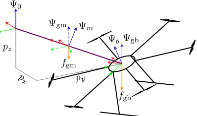
In this study the system is considered as shown in figure 3. The frames introduced in figure 3 are:

Ψ0 inertial non-moving frame which coincides with the

application point;

Ψb UAV body-fixed frame placed in its CoG and aligned

with its principal axes;

Ψm similar to Ψb but for the manipulator;

Ψgb UAV’s gravity frame, also placed in its CoG but

aligned with the axes of Ψ0 such that the

gravita-tional force always points along the negative zˆgb

-axis;

f1 τ1 f2 τ2 f3 τ3 f4 τ4 f5

τ5 _f6

[image:6.612.340.539.57.174.2]

τ6 Ψb la fgb Ψ0 x y z

Fig. 2. Forces and torques generated by-, and gravity working on an under-actuated UAV. The length of the UAV arms is denotedla.

The UAV is treated as a single rigid body that generates the forces and torques as shown in figure 2. These forces and torques can be described as a single thrust force ftalong the

body’sz-axis and three torques about the three body axesτx,

τy, andτz, following

K

   

1 1 1 1 1 1

1

2 1

1 2 −

1

2 −1 − 1 2

−1 0 1 1 0 ₋1

1 ₋1 1 ₋1 1 ₋1

            f1 f2 f3 f4 f5 f6         =     ft τx τy τz    , (2) where

K= diagn1 la

√

3 2 la kd

o

,

and kd 1 is the ratio between generated thrust and drag

torque of the rotors, which is assumed constant and equal for all rotors. la denotes the length between the rotors and the

CoG. For every rotori∈Z∩[1,6], the thrust force of that rotor

isfi∈R∩[0,f¯rot], wheref¯rotis the maximum thrust thatone

rotor can generate. The total thrustftthus isft∈R∩[0,6 ¯frot]

and6 ¯frot= ¯ft.

The torques and force on the right hand side of equation (2) are the controllable inputs of the system.

Besides the inputs, two separate gravitational wrenches are acting in the system. All forces and torques add to the total system wrench as three separate wrenches, expressed as follows

Wb

b = τx τy τz 0 0 ft ,

W_gbgb= 0 0 0 0 0 ₋fgb,

Wgm

gm = 0 0 0 0 0 −fgm,

(3)

where fgb andfgm are the gravitational forces acting on the

UAV body and the manipulator respectively. The frames in which these wrenches are expressed are shown in figure 3.

The generic rigid manipulator is used to transform the wrench generated by the UAV to the application point. To that end, the manipulator can be defined as a generic trans-formation which can be fully described with the H0

b-matrix.

This matrix contains the positionp0

b and orientationRb0of the

Ψ0

pz

p_{x p}y

Ψgm _Ψm

Ψgb

Ψb

fgm

fgb

Fig. 3. Schematic representation of the UAV with generic manipulator. The dashed axes compose the frames for the gravitational forces, the solid axes the body fixed frames. The violet line represents the manipulator.

application point (Ψ0) in the body fixed coordinate systemΨb.

p0

b will also transform the gravitational wrench,

Hgb0 =

I3 p0b

0 1

,

and the gravitational wrench of the manipulator will be trans-formed by halfp0

b

Hgm0 =

I3 1₂p0b

0 1

.

Using equation (1), the wrenches from equation (3) can be transformed to the application point Ψ0. When expressed in

the same frame, the wrenches can be summed element-wise, giving one total wrenchW0

tot.

(W0

tot)T = AdTH0gm(W gm

gm)T+ AdT_Hgb 0 (W

gb gb)T+ Ad

T Hb

0(W b b)T.

To clearly show the dependencies of W0

tot on inputs and

the gravitational forces, it can be expressed as the following matrix product

Wtot0 T

=G τx τy τz ft fgb fgmT, (4)

whereG is a non-linear function of φ, θ, ψ, px,py, and pz

and will be provided in section III-D in simplified form.

B. Constraints and limits

It must be taken into account that the forces in equation (4) are not of the same order of magnitude. fgb is proportional

to the UAV’s mass, thus fixed for a chosen UAV. fgm is

proportional to the length of the manipulator, determined by

px, py, and pz and thus cannot be controlled directly. The

maximum torques τ¯x and τ¯y and the maximum thrust f¯t

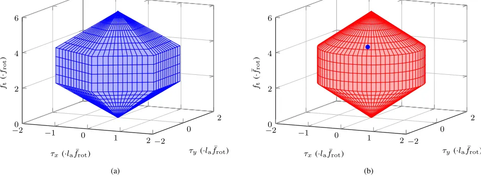
are mutually coupled. This coupling is described elaborately in appendix A. In short, this coupling allows the co-vector

τx τy ftto be in the (approximated) 3D space shown in

figure 13b, assuming that τz is zero. This is captured in the

following inequality constraints

ft+

2 3la

τ _≤6 ¯frot,

2 3la

τ _≤ft, τ≤

3la

2 f¯rot,

where

τ=qτ2 x+τy2

[image:6.612.62.287.59.194.2]

The UAV must be able to maintain in-flight stability with the manipulator equipped. To that end, the additional load torque due to Wgm and the gravitational force acting on the

end-effector cannot be greater than the torque that can be generated with the thrust needed to maintain hovering. To maintain maneuverability, an additional safety factor of 1/2

is used, which places the following constraint on the length and mass of the manipulator

lm,xyg

mee+1

2mm

≤ 3₄lamtotg,

wheremtot=mee+mm+mb,meeis the end-effector mass,

mmis the manipulator mass,mb is the UAV body mass, and

lm,xy is the length of the manipulator projected on the xy

-plane of the world frame, thus the effective arm gravity makes from the end effector’s CoG and the manipulator’s CoG toΨb.

Additionally, the total gravitational force may not exceed

¯

ft/2, again to maintain maneuverability. This places the

following constraint

gmtot ≤1

2f¯t.

Another maneuverability constraint is defined to limit the moment of inertia of the manipulator, including the mass of the end-effector. Due to the relatively low maximum yaw torque about zˆb_{, the additional moment of inertia due to}

the end effector and the manipulator should not reduce the maneuverability too much. When the UAV is in free-flight with the manipulator endowed, there is no need for aggressive maneuvering, but an acceptable angular acceleration must still be feasible. Because angular acceleration is inversely proportional with the total moment of inertia, the maximum moment of inertia about zˆb _{is chosen to be limited to twice}

the moment of inertia of the UAV about zˆb

Jee+Jm≤2Jzz,b,

such that the total moment of inertia aboutzˆb_{remains smaller}

than3Jzz,b.JeeandJmare the moments of inertia of the

end-effector and the manipulator respectively, both about zˆb_{, and}

Jzz,bis the third diagonal element of the UAV’s inertia matrix.

The UAV needs to have a certain distance from the surface on which the torque is applied to safeguard the rotors from hitting the surface. The bounding box of the UAV is approx-imated by a cylinder shape with a radius of la+rr, where

la is the length of the UAV’s arms and rr the radius of the

rotors. An additional safety margin is determined to be 5 cm. The minimum absolute distance |px| from the UAV CoG to

the surface is therefore constraint as

|px| ≥la+rr+ 0.05. (5)

Finally, the maximum angle that the UAV is able to make with the horizontal plane will have to be constraint. For applications in which the manipulator can suddenly break loose from the application point, the UAV must maintain controllability. To that end, the maximum angle is limited by constraining the pitch angleθand roll angleφtoπ/8 = 22.5◦

as follows _p

θ2_+φ2_≤ π

8. (6)

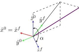
ˆ

x0= ˆxf

ˆ

y0

ˆ

z0

ˆ

yf

ˆ

[image:7.612.370.503.53.141.2]

zf α

Fig. 4. The manipulator (again in violet) without UAV to show howΨf is

defined.

C. Additional wrench frame

Any force generated by the UAV will be directly transferred to the application point. In addition, the transformation of torques fromΨbtoΨ0cannot cancel forces inΨ0. Therefore,

minimizing the force inΨbdirectly minimizes the force inΨ0.

This will bring the optimal manipulator back to where only

τx is exerted on the application point and the thrust is used to

cancel gravity.

To properly define a constraint on the force, it must con-strain the components of the force that are not contributing to the desired torque. To that end, the wrench can be expressed in a virtual frame Ψf, which shares its origin with Ψ0 and

aligns itsyˆ-axis with the projection of the manipulator on the

yz-plane of Ψ0. To transform Wtot0 toΨf, equation (1) can

be used withAdH0 f.

H0

b can be parameterized with six parameters3. The

orienta-tion is parameterized with three anglesψ,θandφ

correspond-ing to the sequential rotations about the zˆ-, yˆ0- and xˆ00-axis

respectively. These angles are Tait-Bryan angles, commonly known as yaw, pitch, and roll in aviation. The three position parameters arepx,py andpz.

Due to the rotational symmetry of the UAV as explained in appendix A, under the assumption that τz is kept zero,

ψ is not influencing the value of W0

tot. Therefore, during

the optimization ψ is taken 0 rad to decrease the needed

computations. Afterwards,ψis taken such that the manipulator

always lies in the xz-plane ofΨb, where x is positive. This

way, the manipulator is always pointing ‘forward’ which will ease flying in free-flight.

Whenpyandpzare known,H0fcan be determined with the

atan2function withpyandpzas arguments. See equation (27)

in appendix D for the definition of atan2 used in this paper.

H0f can then be expressed as

H₀f =

   

1 0 0 0

0 cosα ₋sinα 0

0 sinα cosα 0

0 0 0 1

   ,

where

α= atan2(pz, py).

D. Cost function

The goal of the manipulator is to transform the UAV wrench in such a way that the total wrench in Ψf conforms to the

following:

• τxf is maximized, because this is the goal of this study;

• τyf, τzf, and fyf are minimized, because these torques

are undesired and can damage the end-effector or the application point;

• fxf =fx0is also minimized, but must be positive, because

a positive force along xˆ0 is needed to prevent the UAV

from drifting from the application point. In this, ff

z is not constrained, because it directly contributes

toτf x.

Due to the fact thatkd1, the maximumτ¯zis significantly

smaller than ¯τx and ¯τy. Increasing τz is also very costly

in terms of thrust. Therefore, we choose to neglect τz as a

potential input. Withτz= 0, equation (4) loses a column and

can be expressed as

W0 tot

T

=G τx τy ft fgb fgmT,

whereGis

G=

       

cθ sφsθ pzsφ+pycφcθ −py −p₂y

0 cφ −cφ(pxcθ−pzsθ) px p₂x

−sθ cθsφ −pxsφ−pycφsθ 0 0

0 0 cφsθ 0 0

0 0 ₋sφ 0 0

0 0 cφcθ −1 −1

       

,

wheresiniandcosiare denotedsi andci respectively.

An optimal manipulator can be determined by minimizing an objective function, taking into account the (non-linear) constraints set on the decision variables. The objective function can be defined as

min

qd

QU O(qd)−Oˇ₂,

where

O(qd) = τxf τf fxf fyf T

,

τf =rτyf 2

+τzf 2

, (7)

qd is a vector containing the decision variables, Q ∈ R4×4

is a constant diagonal weighing function, and U _∈ R4×4 is

a diagonal matrix that scales only the force entries of O(qd)

withlm. The latter is used to obtain equal units for all entries,

which allows to sum them in calculating the norm. The desired value ofO(qd)is given inOˇ:

ˇ

O= τb

x,des 0 0 0

T

, whereτb

x,des is the desired target value forτx0.

The following decision variables are combined inqd:

qd= ft τx τy px py pz φ θ.

Two types of constraints are used in the optimization, constant boundary constraints, and inequality constraints. Ad-ditionally, some intermediate variables are used to make the calculations more uncluttered.

The only constant boundary constraint that is of importance is the minimum length ofpx, from equation (5).

px<−(la+rr+ 0.05),

wherela is the length of the UAV arm andrrthe radius of its

rotors. This constraint is limiting themaximumofpx, because

the positivexˆ0_{-axis points into the wall.}

For the following, it is assumed that the manipulator has uniform mass distribution and a mass density per length unit ofρm, the end-effector can be represented as point mass, and

the manipulator as a slender rod.

The intermediate variable values that are calculated are τf

as in equation (7) and

lm= q

p2

x+p2y+p2z,

fgm= gρmlm,

Jee=meelm2,

Jm=1

3mml

2 m,

(8)

whereg is the gravitational acceleration constant.

With the constraints from section III-B and the interme-diate variables from equation (8), the following inequality constraints are set. The inequality constraints are limiting the maximum torque in thexy-plane with equation (9a), the thrust based on figure 13b with equations (9b) and (9c), the total sys-tem weight with equation (9d), the maximum roll/pitch angle combined, with equation (6), and the manipulator moment of inertia, including the end-effector massmeewith equation (9f).

τ−3₂laf¯rot ≤0 (9a)

2 3la

τ₋ft≤0 (9b)

ft−6 ¯frot+ 2

3la

τ ≤0 (9c)

fgb+fgm−3 ¯frot ≤0 (9d) p

φ2_+θ2₋π

8 ≤0 (9e)

Jee+Jm−2Jzz,b≤0 (9f)

The optimization is carried out by using MATLABR _[15],

in particular the functionfmincon4. This function is chosen

to allow for non-linear constraints, using an interior point algorithm for nonlinear programming [16].

E. Results

[image:8.612.393.561.414.533.2]

The numerical values used in this optimization are listed in table I. The value for ρm corresponds to the weight per unit

length of a typical carbon fiber tube. The remainder of values correspond to typical values for a small-scale hexacopter.

For the chosen use case, the desired value ofτb

x,desis chosen

to be 10¯τ which equals 15laf¯rot. Substituting the numerical

values from table I, this equals 60.75 N m, which provides the UAV with enough torque to fasten an M10 metric bolt to its recommended fastening torque.

TABLE I

NUMERICALVALUESUSED IN THEOPTIMIZATIONFUNCTION.

Parameter Value Unit

¯

frot 13.5 N

mb 2.5 kg

la 0.3 m

rr 0.1 m

ρm 0.06 kg m−1

g 9.806 65 m s−2

Jzz,b 0.1 N m s2rad−1

TABLE II

OPTIMALVALUES OF THEDECISIONVARIABLES.

Parameter Value Unit

ft 60.909 N

px −0.45 m

py 1.1807 m

pz 0 m

φ 0 rad

θ 0 rad

τx 2.1636 N m

τy −5.6767 N m

The goal of the optimization is to maximizeτf

x, but keep the

other elements of O(q)close to zero. Because it is unknown

on beforehand what a reachable maximum forτf

x is, the focus

is put on keeping the other elements close to zero. To this end, the weighing functionQis chosen such that less focus is given to the first term of O(q)₋Oˇ.

Q= diag1

2 1 1 1

Interestingly, setting the first element ofQ, henceforth referred to asQ[1], to any value above 0.1, will not change the decision

variables that define H0

b. The decision variables that change

areft,τxb, andτyb. A balance is found between using thrust to

increaseτf

x and consequently increaseτyfor usingτxbandτybto

decreaseτf

y. When settingQ[2]to 0, the maximum thrust will

be used to generate τf

x, because τyf is no longer considered.

The resulting optimal values of the decision variables are listed in table II. These result in a transformationH0

b of

Hb0=    

0.35614 0.93443 0 −0.45

−0.93443 0.35614 0 1.1807

0 0 1 0

0 0 0 1

  

 (10)

and

Hm0 =    

0.35614 0.93443 0 ₋0.225

−0.93443 0.35614 0 0.59035

0 0 1 0

0 0 0 1

  

, (11)

which result in the frames shown in figure 5 as Ψb andΨm

respectively.

As expected, the optimal transformation matrix places the thrust perpendicular to the manipulator arm to maximize its contribution toτf

x. This also ensures thatfyf is zero.

The resulting wrench in the application point then is

Wtot0 = 44.69 10.53 0 0 0 35.65

. (12)

0.2 0 -0.2-0.4

-0.6

-0.2 ₀

0.2 _0.4

0.6 _0.8

1 _1.2

y0 x0

Ψ0 _Ψ

m _Ψ

[image:9.612.50.303.530.647.2]

b

Fig. 5. The optimal transformation ofΨband consequently ofΨm.

The second element can never be zero when the thrust is used to generate additional xˆ0 _{torque, due to the minimum length}

of px. Additionally, in this configuration the last element of

W0

tot is aligned withzˆf and is therefore not constrained. The

first element is nearly 7.3 times as big as¯τ, which comes close to the desired 10 times and is still large enough to fasten an M10 bolt.

The optimal input covector is

τb

x τyb ft≈ 2.2 −5.7 60.9

which is also plotted as in figure 13b. It shows that the endpoint is placed on the surface of the potential space, indicating that the input is completely saturated when applying the maximal torque.

IV. CONTROL

Most possible use cases that require high torques, require it to obtain a certain displacement at high damping or to overcome stiction. The former needs a controller that allows movement and the latter needs a certain amount of caution when increasing the applied torque, due to a possible over-shoot when the friction suddenly decreases drastically. This illustrates that the control of a UAV in torque applying mode is not straightforward and demands a dedicated controller. To achieve this, first the dynamic behavior of the system in the chosen use case is determined. Next a FSM is introduced to overcome the problem of rotating back and forth in the chosen use case. Controllers are tuned for the separate states, and finally the problem of stiction is treated by introducing a FIS to determine an additional controller gain.

A. Dynamics

A dynamic model has been developed to validate the kinematics of the optimal manipulator. Both the UAV and the manipulator are considered rigid bodies, rigidly fixed to each other. For the use case of fastening a bolt, the Degree of Freedom (DoF) that is to be controlled is the rotation about

ˆ

x0_{, which is denoted q}

1. The formerly static transformation

matrices are now functions ofq1 in this use case. The inputs

areft,τxandτy, again assumingτz to be kept zero.

Additionally, a ratchet-like joint is assumed between the manipulator and the bolt. This joint ensures that the UAV is able to move back after tightening the bolt, to keep the needed stroke length small.

twists, the unit twist ofq1is used. The unit twist of a rotational

joint is defined as

ˆ T = ˆ ω ˜

rωˆ

,

whereωˆdenotes the unit angular velocity of the joint andr˜the

tilde representation of the arm rthat reaches from the origin to the rotation axis of ω. Note that this can be any point on that axis [14].

The generalized coordinateq1 only rotates aboutxˆ0, which

gives a unit twist of

ˆ

Tq1 = 1 0 0 0 0 0 T

and a constant Jacobian mapping of

T_i0,0=Jq₉1= ˆTq1q91.

Now this Jacobian can be used to express the kinetic co-energy E∗ _{of the two bodies as follows:}

Ei∗=

1 2

T_ii,0T_IiT_ii,0

=1

2

T_i0,0TAdT Hi

0I i_Ad

Hi 0T

0,0 i

=1

2q9

T_JT_AdT Hi

0I i_Ad

Hi

0Jq9, (13)

whereican be eithermfor manipulator orbfor the UAV and

I denotes the inertia tensor. The choice of expressing every rigid body frame in the CoG of that body with its axes aligned with the principal inertial axes of the body, ensures that _Ii _is

diagonal and can be composed as

Ii₌

Ji 0

0 miI3

.

Besides the kinetic co-energy, the potential energyVi(q)of

every body can be determined as follows

Vi(q) =migh

=mig 0 0 1 0Hi0(q) 0 0 0 1

T

. (14) With equations (13) and (14) the system’s Lagrangian equation can be determined as

L(q1,q91) =E∗(q1,q91)−V(q1)

= 1

2q9

T

1JTAdTHm 0 I

m mAdHm

0 Jq91

+1

2q9

T

1JTAdTHb 0I

b bAdHb

0Jq91

−mmg 0 0 1 0Hm0(q1) 0 0 0 1T

−mbg 0 0 1 0Hb0(q1) 0 0 0 1T

and to that end Hm

0 and H0b must be expressed in terms

of q1. This can be done by transforming the matrices in

equations (10) and (11) as follows:

H0b(q1) =    

1 0 0 0

0 cosq1 −sinq1 0

0 sinq1 cosq1 0

0 0 0 1

    Hb0

−1

,

Hm 0 (q1) =

   

1 0 0 0

0 cosq1 −sinq1 0

0 sinq1 cosq1 0

0 0 0 1

    Hm0

−1 , where H0 b −1 =

(R0

b)T −(R0b)Tp0b

0 1

and likewise for H0 m

−1

.

Euler-Lagrangian equations can be solved for the complete system to find the equations of motion. Substituting the numer-ical values provided by the optimization the Euler-Lagrangian results in

d dt

_∂

L ∂q91

−∂_∂qL =τx0+τtd

3.57q_:1+ 29.39 cosq1=τx0+τtd, (15)

whereτtd denotes the auxiliary torques due to friction.

Due to the aforementioned ratchet joint, the bolt friction torque τb is only considered when the bolt is tightened, i.e.

when q₉1 > 0. Additionally, when the bolt is completely

fastened (when the head of the bolt touches the surface) it will start elongating, adding a spring element to the dynamics. Consequently, the head of the bolt is pulled towards the wall by its elongation, increasing the normal friction of the head. This also increases the friction torques significantly.

τtd=     

0, ifq91≤0,

τb, ifq91>0andxbolt≤0,

τb+τe, ifq91>0andxbolt>0,

(16)

whereτbdenotes the torque due to friction of the bolt andτe

denotes the additional torques due to reaching the end of the bolt. Therefore, there are three separate system models with significantly different dynamic behavior.

To ensure a realistic bolt model, the friction torqueτbcannot

be considered merely viscous. Using a discontinuous friction model that includes a static friction term, can be problematic when using numeric simulation techniques, therefore the con-tinuous friction model from Specker, Buchholz, and Dietmayer is used [17]. Figure 6 shows how the friction force of this rotation can be build from three separate terms, viz. viscous-, Coulomb-, and Stribeck friction. The separate terms can be expressed as:

τv(ω) =Dω,

τc(ω) =τc,ctanh

ω ωt

,

τst(ω) =g(ω) [τst,c−τc(ωsp)−τv(ωsp)],

where

g(ω) = ω

ωsp

exp



₋ √ω

2ωsp !2

+1

2

 

and the total bolt friction torque is

τb(ω) =τv(ω) +τc(ω) +τst(ω). (17)

In the above τc,c andτst,c denote the Coulomb- and Stribeck

friction constants respectively,Ddenotes the viscous damping

constant, andωtdetermines the steepness of thetanhfunction

in the expression for the Coulomb friction. Similarly, ωsp

determines the region in which the Stribeck friction is present. Note thatωsp is notthe Stribeck velocityωst, but is typically

0 ω0

x(rad s−1) τ (N m)

[image:11.612.61.290.58.194.2]

Stribeckτst Coulombτc Viscousτv Totalτb

Fig. 6. Description of a continuous model for the friction forces τb as a function ofω0

x=q91[17].

B. Finite state machine

Due to the significantly different dynamic models resulting from equations (15) and (16), the control approach is chosen to contain a FSM with separately tuned controllers. In state FAS -TENING,q1will start at 0 and rotate toward the desired angle.

When this angle is reached or when the desired application torque is reached, the state will change to ROTATING BACK,

in which the q1 setpoint is set to 0 again. Whenq1 is back at

0, the state will change to FINISHEDif the desired application

torque was reached the last time in FASTENING and back to

FASTENING if the application torque was not reached. Note

that the desired application torque must be smaller than or equal to the maximum torque deliverable.

The inertia of the UAV makes that its angular velocity cannot be changed instantaneously, which means that the switching between states will lower average velocity. Increas-ing the stroke length of the motion thus increases the time efficiency of the control approach. Therefore, the desired position is the maximum q1 provided that the conditions in

section III-D still hold. To that end, the reference setpoint is determined to be π/8 rad, which is the limit of the UAV’s roll/pitch angle.

If the UAV will descend past q1 = 0and reach the end of

the bolt beforebeing rotated back toq1= 0, it is impossible

for the system to return and thus it is stuck in an impasse. To prevent this, the minimum allowed angle is set to 0 and the maximum to π/8. To ensure that overshoot is minimal and movement is smooth, the reference input of the system is chosen to be a third order motion profile.

C. Synthesis

The dynamic equation of motion of the system was derived in section IV-A and is

3.57q_:1+ 29.39 cosq1=τx0+τtd. (18)

The nature of this equation allows the non-linearity of the differential equation to be canceled by an input component. To accomplish that, a feed-forward controller is used. This reduces equation (18) for state ROTATING BACKto

3.57q:1=τx0,

FASTENING

start ROTATING

BACK FINISHED

0/0

-/1

0/0

0/1 1/0

1/0

[image:11.612.316.559.60.191.2]

1/1

Fig. 7. Finite state machine structure of the controller. The conditions are shown in the formhdesired angleq1reachedi/hdesired torqueτx0reachedi,

e.g. 1/0 denotes that the end of the position stroke is reached without reaching the desired torque and 1/1 means that both the desired position and the desired torque are reached. A dash (-) denotes that the concerning state transition can happen with either value for that condition.

representing a moving mass, i.e. a double integrator plant. For the chosen third order motion profile and the considered moving mass, PD controller gains can be determined based on path following criteria [18], [19]. The maximum tracking error is chosen to be 5% of the maximum stroke. The cross-over frequency ωpd of the PD controller is then determined

following

ωpd= s

¯

:

q1√β

¯

et

,

wheree¯tis the desired maximum error andq¯:1is the maximum

acceleration of the third order motion profile, which can be determined as follows:

¯

:

q1=

8hm

t2 m

,

where hm and tm denote the amplitude and the duration of

the motion profile respectively.

The continuous PD controller can be described with the following transfer function

Cpd(s) =Kcτˇzs+ 1

ˇ

τps+ 1

and the parameters can be determined with5

Kc =

meqω2pd

√_β , τˇz=

√ β ωpd

, τˇp=√ 1

βωpd

, (19) whereβ= 10is a tameness factor andmeqis the equivalent

mass as seen by the controller (equal to3.57) [18]. The resulting PD controller is

Cpd(s) =

1.147s+ 5.437 0.02109s+ 1 ,

which is tuned to state ROTATING BACK, where the UAV is moving back with (ideally) zero friction.

Considering that in state FASTENINGthe bolt adds a

com-plex friction component to the dynamics of the system, a different controller is needed. Firstly, there is the possibility

that the end of the bolt is reached just before the end of the

motion profile is reached. The small remaining error will lead to a small plant input, but the large friction torque τe will

immobilize the UAV when only using a PD controller. To reach the end of the stroke or saturate the input without reaching the end of the stroke, an integral action is added.

For a PID controller the desired crossover frequency ωpid

can be determined with

ωpid= 3 s

¯

;

q12β

¯

et

,

where_q¯_{;1is the maximum jerk of the third order motion profile}

[19]. The maximum jerk can be determined with

¯

;

q1=32hm

t3 m

. The PID controller can be described with

Cpid(s) =Kcˇτzs+ 1

ˇ

τps+ 1

ˇ

τis+ 1

ˇ

τis

.

The parameters from equation (19) can be recalculated for the PID controller by substituting ωpd for ωpid and additionally

ˇ

τi can be chosen

ˇ

τi≥2ˇτz

to prevent that the integral action deteriorates the phase advance of the D action[18]. This results in the following PID controller:

Cpid(s) =

0.6045s2_{+ 4.174s+ 5.881}

0.01028s2_{+ 0.5069s} . (20)

To prevent that the state transitions de-stabilize the system, the start of the motion profile when entering a state is set to the current position. Additionally, the I wind-up of the PID controller is reset every state transition.

D. Fuzzy inference system

To generalize the PID controller for state FASTENING for

multiple possible bolt friction shapes, an additional configu-ration gain Ka is used to make the controller adaptive. By

considering the rate of change of q1 and measured torque

on the application point, a convenient choice forKa is made

based on a set of rules that command a FIS. This will allow the controller to e.g. lower Ka when a small force results in

a large rate of change and increase Ka when a large force

results in a small rate of change q₉1.

Ka will scale the controller in equation (20) with a value

between 0.25 and 1.75. The value for Ka as function of q91

and τ is shown in figure 8. The FIS is elaborately discussed

in appendix C.

V. SIMULATION EXPERIMENTS

A. Simulation description

To validate the kinematics of the model derived in sec-tion IV-A, a static simulasec-tion was done with q1 fixed. The

inputs of the model were set to the values in table II. Figure 9 shows a 3D render of the UAV in the optimal configuration.

0 0.2

0.4 ₀ 10 20 30 40 0.4

0.8 1.2 1.6

9

q(rad s−1_{) τ(N m)}

Gain

Ka

[image:12.612.329.554.53.190.2]

0.4 0.8 1.2 1.6

Fig. 8. Evaluation of the FIS with the rules as in appendix C and membership functions as in figure 20.

The total wrench applied to the application point during the static test was

W0

tot= 45.16 10.73 0.00 0.00 0.00 35.71

, (21) which indeed is very close to the optimal value shown in equation (12).

For a dynamic test, the parameters mentioned in equa-tion (17) must first be determined. The needed accuracy for these parameters is low, therefore it is sufficient to make a rough approximation of the order of magnitude of the parameters. By initializing the UAV in the optimal state and setting the input to zero, it should intuitively behave as a damped pendulum. The parameters have been set such that the response was roughly equal to that of a physical damped pendulum. It will be shown later that a high accuracy for these parameters is not significant for the validation of the optimal manipulator and derived controller.

To ensure that the FSM controller works as intended for a variety of possible bolts, the bolt friction torque τb is scaled

between 1/2 and 3/2 times its initial value.

B. Results

Three simulations have been run, with τb scaled by 1/2,

1, and 3/2 respectively. Figure 10 shows the results of these three simulations, i.e. in- and output of the plantuandq1, the

reference angleq1,des, the error between reference and output

e, the applied torqueτx0 and the additional controller gainKa

as returned by the FIS. The latter is set to 1 if the FSM is not in state FASTENING. Note that the inputuis normalized with the maximum torque from equation (12).

As can be seen in figure 10, the differences between the different scalings of the bolt friction torque are marginal. The simulation with 3

2τˆbshows that the increased Stribeck friction

causes the FIS to return a higher additional gain to overcome this friction. The simulation with 1

2τˆb shows that overall the

additional gain is lower.

For all three simulations, att∗_{the end of the bolt is reached}

and the elongation and additional friction enforce that the UAV can no longer follow the motion profile accurately. This causes the error signal to rise, consequently increasing uuntil it is

saturated. When u is saturated for some nonzero time, the

controller switches to ROTATING BACK, moves back toq1= 0

Ψm _Ψ 0

ft

fgb

Ψb

(a)

Ψm

Ψ0

Ψb

(b)

Ψm _Ψ

0

ft

fgb

Ψb

[image:13.612.47.301.54.505.2]

(c)

Fig. 9. A 3D rendering of the UAV with the optimal manipulator, during the static simulation test. (a) shows an overview, (b) shows a top view fromzˆb_,

and (c) a front view from−ˆx0_.

VI. DISCUSSION

Without constraints on φ and θ, the optimal state would

be when the thrust ft and gravity fgb pointed in the same

direction, thus with the UAV placed upside down. In this study it is assumed that this state would be an unacceptable risk for the system and therefore φandθhave been limited.

The second element of the optimal wrench in equation (12), i.e. the applied τ0

y, is nearly one fourth of the desired τx0.

Due to the maneuverability constraints, the length of the manipulator is limited. Additionally, the bounding box of the UAV places a minimum onpx. The combination of these two

constraints leads to the significantτ0

y that can only be canceled

by the UAV’s τb

y or τxb. These torques again are limited due

to the coupling of the thrust and the torques as described in appendix A. Consequently, to decrease τ0

y, τx0 will have to

Bolt

pos.

xblt

(mm)

FASTENING ROTATING BACK

1

2ˆτb ˆτb

3 2τˆb

−0.1

−0.05 0

Angle

q1

(rad)

0 0.2 0.4

Error

e

(rad)

−0.1 0 0.1

Ref.

q1,

des

(rad)

0 0.2 0.4

Gain

Ka

0.5 1 1.5

Torque

τ

0 x

(N

m)

0 100 200

Timet(s)

Plant

input

u

0 2 4 6 8

−1 0 1

[image:13.612.322.560.55.698.2]

t∗

Fig. 10. Simulation results of the dynamic simulations. Three tests have been conducted, with 3

2ˆτb,τˆb, and 12ˆτb. The jumps in the reference signal are due to the switching between states. The applied torque shows a similar spike for all three simulations, although the one for 3

decrease too. A proper balance between these torques can be found by adjusting the weighting functionQ. For the use case considered in this study, the value of τ0

y is acceptable.

Interestingly, the optimal transformation matrix H0 b stays

the same for any value above 0.1 forQ[1]. Even when changing

Q[2] to 0, thus omitting the penalty onτy0, results in the same

H0

b. It seems that the transformation matrix is optimized to a

global minimum of the cost function, within the set constraints. The optimal rollφand pitchθangles are zero, which positions

the thrust direction perpendicular to the effective arm of the manipulator. Consequently this ensures that ff

y = 0 and that

all thrust force is contributing to τ0 x.

When setting Q[2] to 0,τxb and τyb will no longer be used

and the maximum thrust is used to generate τ0

x, because

τf

y is no longer considered. With the optimization results in

section III-E, the target torque of 60.75 N m is not reached, but the obtained torque is near to being considered extreme, following the definition in section II-A.

As shown in figure 13b, the endpoint of the input covector is placed on the surface of the potential space. More specifically, it is placed on the top face, which indicates that the input covector is fully saturated. When changing Q, the endpoint will move over this face but will remain coincident. Only when Q[1] is smaller than 0.1, R0b will be identity and p0b

will be −0.45 0 0T. The thrust is then used to cancel the

gravitational force and only the intrinsically generated τb x is

transferred to the application point. The endpoint of the input covector is still located on the surface of the potential space in figure 13b, but on the middle cylinder section.

Considering the maximum thrust of the specific UAV and the length of the optimal manipulator perpendicular to the xˆ0

axis, the theoretically maximum torque τ0

x would be

( ¯ft−fgb) q

p2

y+p2z≈66.7 N m

and the unwanted maximum torqueτy0 would be

( ¯ft−fgb) p

p2

x+p2z≈25.4 N m.

The achieved torqueτ0

x of 44.7 N m andτy0of 10.7 N m reach

approximately 67% of the theoretical maximum τ0

x and only

41% of the undesired theoretical maximum τ0 y.

Considering the controller, the FIS to determine Kc adds

complexity to the control system, but also contributes greatly to the performance. In comparison with a conventional PD controller, tuned for both state FASTENING and ROTATING BACK, the FIS FSM shows less overshoot, a better tracking of

the motion profile, and a better response on stick-slip behavior. On the other hand, the structure of the controller is still P(I)D tuned for a relatively slow motion profile. An alternative might be to tune a P(I)D controller such that it is critically damped when applied to the considered system. Supplying a step reference input to the controlled system would prevent overshoot and offer high immediate gain due to a large immediate error. The slow initial increase of the currently applied motion profile leads to a longer time period where the Stribeck friction is active. Due to this slow start the controller has to catch up when the Stribeck friction is overcome, still causing some overshoot.

The torque curve in figure 10 shows three minor peaks: one at the start and two more at the two first state transitions. This additional torque is probably required to overcome the Stribeck friction component. The higher Stribeck friction for the simulation where τb = 3₂τˆb, seems to cause a stick-slip

behavior after the second state transition. This in turn causes

Kato increase quickly, but considering the curves of the plant

inputuand the errore, it seems to overreact.

At the point in time when the bolt hits the end of its thread, t = t∗ _{in figure 10, a significant spike is detected}

in the applied torque τ0

x which exceeds the torque of the

optimal wrench excessively. This could indicate that even higher application torques could be achieved by building up the UAV’s momentum and transferring it in a short time interval to the application point. In a real-world test this spike will probably be tempered by the internal damping of the bolt, which is not considered in this simulation.

The additional gainKa was expected to change smoothly

with varying damping in state FASTENING due to its

con-tinuous shape shown in figure 8, but in simulation it changes erratic. This might be due to the inputs of the FIS. One input is the measured torqueτ0

x, which changes almost instantaneously

with adjusting Ka. The other input is the rate of change 9

q1, which needs time to change due to the UAV’s inertial

properties. This could cause the following development ofKa

during simulation: 1) τ0

x is normal and q91 is still zero initially

2) This causesKato increase, in turn increasingτx0

instan-taneously

3) q91does not change directly, but the measuredτx0is larger

than during the former time step

4) This causes Ka to increase more, increasing τx0 more

too

5) Repeating 2-4 causes Ka to quickly reach its limit

The same reasoning can be followed for whenq91 is too small

andKa is quickly decreased.

VII. CONCLUSION

In this paper the initial steps have been taken towards the application of extreme interaction torques with underac-tuated UAVs. The kinematics have been derived of a generic transformation of the UAV. Constraints for the optimization algorithm have been determined based on input saturation, maneuverability, and safety margins. A optimization algorithm has been designed that takes the desired torque τ0

x, the UAV

parameters, and a weighting function as input and derives the optimal H0

b matrix and input covector to achieve that

torque taking into account the weighting of the desired and the undesired forces and torques.

state, both in addition to a feed-forward controller canceling the gravitational influence. The PID controller is adaptive by means of an additional gain, which is determined by means of a Fuzzy Inference System (FIS) based on current angular velocity and torque.

The controlled system has proven to be able to fasten a variety of bolts with different friction parameters. The FIS has proven to successfully counteract the complex nonlinearity of the bolts friction model, but its performance can probably be improved with other semantic rules that prevent the quickly increasing or decreasing resultingKa.

The optimal manipulator and input covector of the UAV balance the desired and undesired wrench elements inΨ0and

achieve a τ0

x of 67% of its theoretical maximum and aτy0 of

only 41% of its theoretical maximum. For the specific UAV, the achieved τ0

x is more than 7 times larger than the torque

that it can generate intrinsically.

A. Future work

This study was focused on achieving a static maximum torque. Future work can use the optimization of the manipu-lator as presented and possibly further increase the achievable torque by utilizing the dynamic properties of the UAV. For example, the inertia and mass of the UAV can be used as a momentum storage, increasing momentum by building up (angular) velocity. This momentum can be transferred to the application point in a short time interval, to achieve a resulting torque that can be added to the static torque achieved in this study.

Another possible addition to this area of study could be the application of a powerful external actuator on the end effector of the manipulator. Using the powerful actuator and the ‘slowness’ of the UAV’s inertia, a short powerful torque could be applied to the application point.

APPENDIXA

COUPLING BETWEEN THRUST AND TORQUE

Underactuated UAVs use the thrust from multiple parallel rotors to directly control their altitude and attitude. The altitude can be directly controlled by increasing or decreasing all thrusts. To control attitude, torques about the body fixedxˆb_,yˆb_,

andzˆb _{can be generated, which follow from the rotor thrusts}

and the UAV motor layout.

For a hexacopter as shown in figure 11, these four forces are expressed in the rotor thrusts as follows:

T =f1+f2+f3+f4+f5+f6 (22)

τx=la(f2−f5) +

1

2la(f1+f3−f4−f6) (23)

τy=

√

3

2 la(f3+f4−f1−f6) (24)

τz=kd(f1−f2+f3−f4+f5−f6) (25)

Three (symmetric) limits can be recognized when express-ing the thrust T as a function of τx and τy, as shown in

figure 12. The point (0,0) in figures 12a and 12b can be found by noticing from equation (22) that at zero thrust, all fi must

be zero, thus from equations (23) and (24) follows thatτxand

1

2

3 4

5 6

x

y

la

Hexagon formed by the rotors

Possible space for τx τy ft, viewA

Approximated space for τx τy ft Fig. 11. UAV motor layout for a generic hexacopter.

τyare also zero. The line segment to point (1.5,2) can be found

by maximizing the torque with the minimum amount of thrust. The segment from point (1.5,2) to point (1.5,4) follows from the fact that the torque is kept the same if the forces on both sides of the axis are increased equally. The maximum thrust in (0,6) can be found by increasing all forces to their maximum. The total thrust is then6 ¯frot, but the forces in equations (23)

and (24) cancel out so there is no torque. The limits can be mirrored inzˆ, completing the symmetric shape whereinT and τx can be controlled.

Forτy this shape is similar, but stretched out in horizontal

direction. This is due to the fact that the average arm length at maximum τx is only 3/2la which is slightly smaller than

the average arm length at maximum τy of √3la≈1.73la.

A virtual axis running through rotor 1 and 4, or through rotor 3 and 6, has the same thrust-torque space as the yˆ

axis. Similarly, the axes perpendicular to these mentioned axes have the same thrust-torque space as the xˆ axis. By linearly

interpolating between these six planes, the three-dimensional thrust-torque space can be defined as shown in figure 13a.

The space in figure 13a can be approximated by a rota-tionally symmetric space, which is obtained by rotating the shape in figure 12a about the τx = 0 line. This gives the

largest rotationally symmetric space that fits in the space of figure 13a.

APPENDIXB

BOND GRAPH MODEL

Modeling the dynamic equations of section IV can be done graphically by means of (multi) bond graphs in conjuncture with screw theory. For an introduction in bond graph theory, readers are referred to [20]. The models in this section were derived using bond graph terminology and the simulations from section V have been done using 20SIMR _{[21] in}

combi-nation with the controller in MATLABR _[15].

In the figures provided in this section, the port s1 denotes

A A

−3

2 −34 34 32

2 4 6

τx(·laf¯rot)

ft(·f¯rot) I II III

(a)

A A

−√3 −1 2

√

3 1

2

√

3 √3

2 4 6

τy(·laf¯rot)

ft(·f¯rot) IV V VI

(b)

x

y z

la

f4+f6 f5

(c)

x y z

√

3 2 la

f3+f4

(d)

x

y

z _f

1+f3

f4+f6

f5

(e)

x y

z f3+f4 f2+f5

(f)

x

y

z _f

2

f1+f3 f4+f6

f5

(g)

x y

z f3+f4 f2+f5 f1+f6

[image:16.612.63.517.58.483.2]

(h)

Fig. 12. Graphical representation of the dependency of T onτxandτy. The graph in (a) shows the plotted relation. (c), (e) and (g) show (in orange) the

thrust changes that follow the line segments of I, II, and III in (a) for positiveτxrespectively, and (in violet) the corresponding torque change. For negative τx, the thrusts are identical, but mirrored inˆz. Similarly, (d), (f) and (h) show the thrust changes that follow the line segments of IV, V, and VI in (b) for

positiveτyrespectively, and the corresponding torque change. Note that the maximumτyis slightly bigger thanτxdue to the longer average arm length.

−2 ₋₁

0 ₁

2 −2 0

2 0

2 4 6

τx(·laf¯rot) τy(·laf¯rot)

ft

(

·

¯_frot

)

(a)

−2 ₋₁

0 ₁

2 −2 0

2 0

2 4 6

τx(·laf¯rot) τy(·laf¯rot)

ft

(

·

¯_frot

)

(b)

[image:16.612.67.542.533.708.2]

(p) output (square) numbered 2. These ports have no dynamic behavior and only transmit either a signal or a (multi) flow-effort pair.

The high level model in figure 14 consists of a UAV

-block, which holds a rigid body bond graph structure with a modulated source of effort for the input force and torques [22]. The Joint-block contains a bond graph generic joint, but

without degrees of freedom, effectively fixing the manipulator in the Body-block to theUAVwith a high stiffness and high

damping.

The Bolt-block is shown in figure 15 and theRatchet

-block is shown in figure 16. The former consists of a switching

X1-junction that switches closed when the end of the bolt’s

thread is reached. The latter is used as sensory input for the controller and holds a dissipative element that is switched on when q91>0 and switched off otherwise.

UAV p1

s1

Joint

p1

p2

s3

FSM

s1

s2

Ratchet p4

p5

s2

Manipulator

p2

p3

s3

Bolt

[image:17.612.352.519.66.166.2]

p5 RC

Fig. 14. The high level block diagram of the dynamic model.

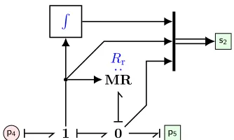
1 MR

Rb(q91)

:

I

Jbolt

:

p5 TF

λ

:

X1

x <0

:

1 MR

Re(q1)

:

C

1 Ke:

Fig. 15. Bond graph of theBolt-model.

p4 1 0

MR

Rr_:

p5 R

s2

Fig. 16. Bond graph of theRatchet-model.

p1 0 p2

MTF H0

j =Hb0Hjb

:

s3

[image:17.612.66.548.186.720.2]

1 RC

Fig. 17. Bond graph of theJoint-model.

1 MSe

τb

x τyb ft

:

I

Ib

:

RTF

Hb gb

:

MTF Hb

0

:

1 p2

MGY

−adT

T_bb,0 P bT

:

Se

W_gbgb: s1

Fig. 18. Bond graph of theUAV-model.

1 I

Im

:

RTF

Hm gm

:

MTF Hm

0

:

1

p2 p3

MGY

−adT

Tmm,0(P

m₎T

:

Se

Wgm gm :

s3

[image:17.612.66.276.257.557.2]

0 5 10 15 20 25 30 35 40 45 Measured torqueτ(N m)

0 0.1 0.2 0.3 0.4 0.5 0

0.5 1

SM LA

Angular velocityq9(rad s−1)

De

gree

of

membership

[image:18.612.58.264.57.205.2]

µ

Fig. 20. Membership functions of the input of the Fuzzy Inference System (FIS).

APPENDIXC

FUZZYINFERENCESYSTEM

A Fuzzy Inference System (FIS) is used to adjust the proportional gain of the PID controller in state FASTENING, due to the unknown friction of the bolt when tightening. The friction cannot be measured directly, therefore the gain is adjusted based on the rate of change of q1 and the measured

torque on the application point. Four straightforward semantic rules are used to determine Ka, which is used to scale the

gainKc of the PID controller. These rules are of the structure

IF (antecedent) THEN (consequent):

1) If q₉1=LA andτ =SMthenKa = 0.25

2) If q₉1=LA andτ =LAthenKa = 0.75

3) If q₉1=SM andτ =SMthenKa = 1.25

4) If q91=SM andτ =LAthenKa = 1.75

In order of the list above, if the current velocity isLA, although

the measured torque is SM, the friction of the bolt is most

probably small. In that case the control signal can and should be lowered to prevent that the UAV will overshoot its setpoint. If both the measured torque and the current velocity are LA,

the gain can be slightly lowered, because the velocity should be limited. If both signals areSM, the gain is slightly increased

to help overcome the Stribeck friction of the bolt. If on the other hand the current velocity isSMand the measured torque

is LA, the friction is probably high. In that case, the control

signal can be increased within the limits of what the UAV is able to apply.

The membership functions that correspond to the values

SM (small) and LA (large) for the input signals are shown

in figure 20. Note that the scale for the measured torque is shown on the top x-axis. The surface plot in figure 8 shows

the evaluation of the FIS for the possible combinations of τ

andq91.

The Gaussian membership functions are described by

µ(x) = exp

−(x₋c)2

2σ2

, (26)

where σ is chosen τ /¯ 4 = 11.25 for the torque membership

functions and_q¯_{91/4 = 0.125for the rate of change membership}

functions. The constant c is the value of x where the center

of the Gaussian function is located. ForSM this is atx= 0, for LAthis is atx= ¯x.

A. Example

For a given pair(q₉1, τ), the corresponding value forKa can

be determined as follows. Firstly, the degree of membership

µfor all membership functions is determined as follows:

µτ,SM(τ) = exp

−τ2

2(τ¯ 4)2

= exp

−τ2

253.125

,

µτ,LA(τ) = exp

−(τ₋¯τ)2

2(τ¯ 4)2

= exp

−(τ₋45)2

253.125

,

µq91,SM(q91) = exp −9

q2 1

2(q¯91 4)2

!

= exp

−q92 1

0.03125

,

µq91,LA(q91) = exp −(q91−

¯₉

q1)2

2(q¯91 4)2

!

= exp

−(q91−0.5)2

0.03125

. Then the fuzzy logic value of the antecedents in the FIS rule-set are determined. The fuzzy logic equivalent of the logical

ANDis to take the minimum of the two degrees of membership

as follows:

a1= min(µq91,LA, µτ,SM), a2= min(µq91,LA, µτ,LA), a3= min(µq91,SM, µτ,SM), a4= min(µq91,SM, µτ,LA).

Then the resulting value ofKa can be determined with

Ka = 4 P i=1

aici

4 P i=1

ai

,

whereci are the consequents as given by rule 1 to 4.

APPENDIXD

DEFINITION OF ATAN₂

In this study, the following definition for theatan2function

is used:

atan2(y, x) =                   

atan y_x for x >0,

atan y_x+π for x <0 andy_≥0,

atan y_x−π for x <0 andy <0,

π

2 for x= 0 andy >0,

−π

2 for x= 0 andy <0,

0 for x= 0 andy= 0

(27)

REFERENCES

[1] D. R. McArthur, A. B. Chowdhury, and D. J. Cappelleri, “Design of the I-Boomcopter UAV for environmental interaction,” in2017 IEEE International Conference on Robotics and Automation (ICRA), May

2017, pp. 5209–5214.DOI: 10.1109/ICRA.2017.7989611.

[2] G. Heredia, A. E. Jimenez-Cano, I. Sanchez, D. Llorente, V. Vega, J. Braga, J. A. Acosta, and A. Ollero, “Control of a multirotor outdoor aerial manipulator,” in 2014 IEEE/RSJ International Conference on Intelligent Robots and Systems, Sep. 2014, pp. 3417–3422.DOI: 10. 1109/IROS.2014.6943038.

[3] A. Mirjan, F. Gramazio, M. Kohler, F. Augugliaro, and R. D’Andrea, “Architectural fabrication of tensile structures with flying machines,”

Green Design, Materials and Manufacturing Processes, pp. 513–518,