Improving the prediction of pressure gradient field in wind farm numerical simulation method, WAKEFARM

(1)

1

Faculty of Engineering & Technology

Improving the prediction of pressure gradient field in

wind farm numerical simulation method, WAKEFARM

Gopala Krishnan Sankara Subramanian Sustainable energy technology

M Sc. Thesis October 2018

EFD-293

Supervisors:

(2)

(3)

Assessment committee

Supervisor

dr.ir.Arne van Garrel

Engineering fluid dynamics, University of Twente

Chairman

Prof.dr.ir.C.H.Venner

Engineering fluid dynamics, University of Twente

Supervisor from company ir. Edwin Bot

Researcher, wind energy

Energy research centre of the netherlands

External member dr. Maarten.J. Arentsen

Faculty of Behavioural, Management and Social Sciences University of Twente

(4)

(5)

Abstract

The wind turbines in a wind farm interact aerodynamically through their wakes. The wakes are characterized by reduced wind speeds and increased turbulence. These wake effects influence the overall power production of the wind farm and cause ad-ditional fatigue loading. The numerical modelling of wind farms is vital, as it helps us to understand the wind turbine wake interactions and to predict the total power output of the wind farm better. The current wake model at the Energy research Centre of the Netherlands is implemented into a Fortran code named WAKEFARM. It simulates the wake properties of a single turbine or a row of turbines. WAKE-FARM solves Reynolds averaged Navier Stokes equations in perturbation form. The Reynolds averaged Navier Stokes equations used in WAKEFARM are parabolized in the streamwise direction. The two momentum equations in the transverse direc-tions are elliptic and are solved iteratively. The axial pressure gradient in the axial momentum equation is neglected in the far wake and prescribed along with the body force, in the near wake. This axial pressure gradient is calculated using an inviscid vortex models. The induced velocity vectors calculated from the vortex model are given as initial guesses to the perturbation variables in the three momentum equa-tions. In this thesis work, two vortex methods that give an improved prediction of the pressure gradient field are developed: model of a wind turbine rotor with more than three blades with span varying circulation and constant axial induction along the span and a model of a real wind turbine having three blades with span varying circulation and axial induction distributed along the span. Both the models trail a helical wake. The root vortex is included in both the models. The axial pressure gra-dient is calculated from inviscid, incompressible Navier Stokes equations. The trend in the calculated axial pressure gradient is in good agreement with the momentum theory. The two new near wake models (vortex models) are implemented in WAKE-FARM. The horizontal velocity profiles in the cross-flow direction at hub height are validated with field measurements in ECNs wind turbines test site in wieringemeer. The constant axial induction model correlates well with the experiments compared to the existing vortex models. The implementation of the root vortex was successful. The new method shows a flattened velocity profile near the centre of the wake, due to the influence of root vortex. The centerline velocity profiles are validated with wind

(6)

(7)

List of Figures

2.1 Different regions in the wake of a wind turbine . . . 6

2.2 Coordinate system used in WAKEFARM . . . 7

2.3 Pressure and Velocity distributions in actuator disk model . . . 12

2.4 Profiles of the length scale for neutral conditions with boundary layer height of1000mand roughness lengthz0 = 0.05mThe dashed-dotted line correlates to the surface layer scaling. The dashed line includes the effect of first two terms and the full line includes the effect of all three terms in the formulation of the length scale [1]. . . 16

2.5 Computational domain iny−z plane in WAKEFARM [2] . . . 18

2.6 First step in ADI method . . . 19

2.7 Staggered grid . . . 20

2.8 SIMPLE method [3]. . . 20

2.9 Comparison of horizontal velocity profile in the cross flow direction at hub height and at downstream distance 2.5D with EWTW mea-surements. The axial induction factor at rotor a = 0.245 and the free stream velocity at hub height is11m/s . . . 22

2.10 Comparison of centerline velocity profile at downstream distance of x−5D with Marchwood experimental data. The thrust coefficient at the rotorCt = 0.62 . . . 22

3.1 Wake represented as a vortex tube [4] . . . 24

3.2 Model of wind turbine wake with discrete ring vortices . . . 25

3.3 Resolving the vortex density on the surface of a single tip vortex into its axial and tangential components[5]. . . 25

3.4 Side view of trailing helices, for different tip speed ratios.λ= 6(left),λ= 9(right) . . . 28

3.5 Helical wake structure behind a wind turbine . . . 30

3.6 Geometrical parameters of a helical filament . . . 30

3.7 Vortex system in a single bladed wind turbine. . . 32

3.8 Representation of helix by straight vortex segments, the helix has a radiusr0 and length7.5D . . . 33

(12)

3.9 Schematic for Biot Savart law [6]. . . 34 3.10 Non-dimensional wake radius calculated from Oye’s vortex ring model

[5], as a function of distance from the turbine for an axial induction factor, a= 0.33 . . . 37

3.11 Trailed vorticity distribution along the blade span . . . 37 3.12 Bound circulation distribution along the lifting line corresponding to an

axial induction factor,a = 0.33 . . . 38

3.13 The horizontal velocity profile in the cross flow direction at hub height for a free stream velocity of11m/s at a distance of2.5Ddownstream

of the rotor. . . 38 3.14 Normalized horizontal velocity profiles in the cross flow direction at

hub height for an axial induction factor a of 0.33 at various locations

downstream of the wind turbine rotor. The parameters used are Nb =

6,Nr = 25,Nh = 318 . . . 39

3.15 The horizontal velocity profile in the cross flow direction at hub height for an axial induction factor,aof0.33at a distance of2.5Ddownstream

of the rotor, for Nb = 3,6,12,24,48,96withNr = 25andNh = 320 . . . 40

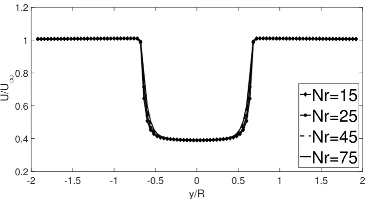
3.16 The horizontal velocity profile in the cross flow direction at hub height for an axial induction factor,aof0.33at a distance of2.5Ddownstream

of the rotor. The number of span-wise vortex filaments are Nr =

15,25,45,75withNh = 320andNb = 6 . . . 40

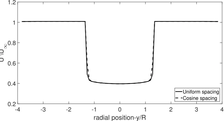
3.17 The horizontal velocity profile in the cross flow direction at hub height at a distance of 2.5D downstream of the rotor obtained using cosine

and uniform spacing. . . 41 3.18 Bound circulation distribution along the lifting line obtained using

co-sine and uniform spacing . . . 41 3.19 Axial pressure gradient at hub-height and centre of nacelle as a

func-tion of distance downstream of the turbine . . . 43 3.20 Bound circulation distribution along the lifting line corresponding to an

axial induction factor, a= 0.33and Root radius, Rr = 6.2m (left),Rr =

2.5m(right) . . . 44

3.21 Trailed vorticity distribution along lifting line corresponding to an axial induction factor,a = 0.33andRr = 6.2m(left),Rr = 2.5m(right). . . 44

3.22 The horizontal velocity profile in the cross flow direction at hub height for an axial induction factora= 0.33and root radius, Rr = 6.2m (left),

Rr = 2.5m (right) at a distance of 2.5D downstream of the rotor. A

(13)

LIST OF FIGURES XIII

3.23 Normalized horizontal velocity profiles in the cross flow direction at hub height for an axial induction factora of0.333 at various locations

downstream of the wind turbine rotor. A hundred points were used

along the scan line. The root radius is taken as6.2m . . . 45

3.24 The hub designs in Enercon (left) and GE (right) blades [7]. . . 46

3.25 Axial induced velocities in theX−Z plane and Y = 0for an uniform free stream velocity of11m/sand axial induction factora = 0.245. The root radius is selected as6.2m . . . 47

4.1 Velocity triangle in a wind turbine blade . . . 50

4.2 normal vectors in a wind turbine blade . . . 51

4.3 Flow chart of the lifting line algorithm . . . 53

4.4 Distribution of lift coefficient,Clalong the lifting line . . . 54

4.5 Distribution of bound circulation,Γb along the lifting line . . . 54

4.6 Distribution of local induction factor,a along the lifting line . . . 55

4.7 Distribution of angle of attack,αalong the lifting line . . . 55

4.8 Horizontal velocity profile in the cross flow direction at hub height at rotor plane. Number of points along the scan line is100 . . . 55

4.9 Horizontal velocity profile in the cross flow direction at hub height and atx−2.5D. Number of points along the scan line is100 . . . 56

4.10 Distribution of local axial induction factor, a, along the lifting line for two different values ofNr. . . 56

4.11 Distribution of lift coefficient,Cl, along the lifting line for two different values ofNr. . . 57

4.12 Horizontal velocity profile in the cross flow direction at hub height and atx = 2.5D for two different values ofNr = 18,36. Number of points along the scan line is100 . . . 57

4.13 Horizontal velocity profile in the cross flow direction at hub height and at x = 2.5D predicted by two different rotor models, constant axial induction model, and radially varying axial induction model. Hundred points were used along the scan line . . . 58

4.14 Horizontal velocity profile in the cross flow direction at hub height and rotor plane predicted by two different rotor models, the constant axial induction model, and radially varying axial induction model. Hundred points were used along the scan line . . . 58

4.15 Axial pressure gradient at hub-height and aty= 0.5Ras a function of distance downstream of the turbine . . . 59

(14)

5.2 Top view of EWTW experimental setup. In yawed conditions, the met mast shifts along the dashed line with respect to the rotor. . . 62 5.3 Horizontal velocity profile in a single wake at x-2.5D measured at

EWTW site for 3 ambient wind speed classes [8]. . . 63 5.4 Horizontal velocity profile at x-3.5D behind the rotor, measured at

EWTW site for 3 ambient wind speed classes [8]. . . 63 5.5 Comparison of horizontal wind speed profiles predicted by three

dif-ferent near wake models at hub height andx= 2.5D, for a wind speed

of11m/s. The root radius is taken as2.5m . . . 65

5.6 Comparison of horizontal wind speed profiles predicted by three dif-ferent near wake models at hub height andx= 3.5D, for a wind speed

5.7 Comparison of horizontal wind speed profiles predicted by three dif-ferent near wake models at hub height andx= 2.5D, for a wind speed

5.8 Comparison of horizontal wind speed profiles predicted by three dif-ferent near wake models at z=hub height and x = 3.5D, for a wind

speed of11m/s. The root radius is taken as6.2m . . . 66

5.9 Horizontal wind speed profiles at hub height, predicted by helical model at various x−2.5D downstream of the turbine for 3 different

values ofNb = 3,6,12and forNr = 25, Nh = 320. The wind speed at

hub height is11m/s. The root radius is taken as2.5m. . . 67

5.10 Horizontal wind speed profiles at hub height, predicted by helical model at various x-locations downstream of the turbine. The wind

speed at hub height is 11m/s. The root radius is taken as6.2m . . . . 68

5.11 Local axial induction distribution along the blade. . . 69 5.12 Comparison of horizontal velocity profiles at x = 2.5D predicted by

constant axial induction model and radially varying axial induction with EWTW experiments. The parameters used in the both the helical modelsNh = 320, Nb = 3, Nr= 36. . . 70

5.13 Comparison of horizontal velocity profiles at x = 3.5D predicted by

constant axial induction model and varying axial induction with EWTW experiments. The parameters used in the both the helical models

Nh = 320, Nb = 3, Nr = 36 . . . 70

5.14 Free-stream velocity u0 profiles obtained from Panofsky-Dutton and Gryning models. The free stream velocity at hub height is 11m/s. . . . 71

5.15 Horizontal velocity profiles along z-axis at x = 5D, y = 0 obtained

(15)

LIST OF FIGURES XV

5.16 Comparison of horizontal wind speed profiles at z=hub height andx= 2.5D, predicted by the WAKEFARM method using Panofsky-Dutton

and Gryning models for a wind speed of 11m/s. The root radius is

taken as2.5mandNb = 12. . . 72

5.17 Comparison of horizontal wind speed profiles at z=hub height andx= 3.5D, predicted by the WAKEFARM method using Panofsky-Dutton and Gryning models for a wind speed of 11m/s. The root radius is taken as2.5mandNb = 12. . . 73

5.20 Velocity deficit inx−z plane and at y = 0 obtained using Panofsky-Dutton ABL model. . . 75

5.21 Velocity deficit inx−z plane and aty= 0obtained using Gryning ABL model. . . 75

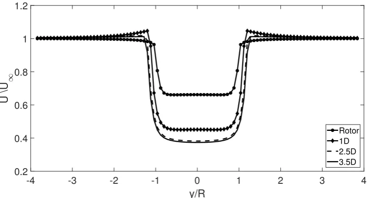
5.22 Comparison of centerline velocity profiles predicted by three different near wake models at5Ddownstream of the turbine. . . 77

5.23 Comparison of centerline velocity profiles predicted by three different near wake models at7.5Ddownstream of the turbine. . . 77

A.1 Conventions in vortex ring model . . . 85

B.1 power and thrust coefficient curves as function of wind speed for the selected wind turbine [9]. . . 87

B.2 Chord distribution in the selected wind turbine. . . 88

B.3 Twist distribution in the selected wind turbine. . . 88

B.4 FFAW3-211 airfoil [10] . . . 89

B.5 FFAW3-241 airfoil [10] . . . 90

B.6 FFAW3-301 airfoil [10] . . . 90

B.7 NACA63-218 airfoil [10] . . . 90

B.8 NACA63-221 airfoil [10] . . . 91

B.9 The lift coefficient Cl as a function of angle of attack α for the five different airfoils . . . 91

(16)

(17)

List of Tables

2.1 Stability classification based on Monin-Obukhov length(L) . . . 17

3.1 Input parameters . . . 36

3.2 Input parameters for modelling root vortex . . . 44

3.3 Input parameters used to simulate the wind turbine. . . 46

4.1 Properties of the selected wind turbine . . . 52

4.2 Input parameters used for simulation of the selected wind turbine blade 52 5.1 Inputs parameters to WAKEFARM wake model. . . 64

5.2 Input parameters to the helical wake model . . . 64

5.3 Input parameters for comparison of constant axial induction and vary-ing axial induction model . . . 69

5.4 Input parameters for Panofsky-Dutton and Gryning test cases. . . 71

5.5 Inputs parameters to WAKEFARM . . . 76

5.6 Input parameters to the constant axial induction -helical wake model . 76 B.1 generic aerofoil properties for the selected wind turbine . . . 89

(18)

(19)

(20)

List of Symbols

Symbols Description Units

a Axial induction factor in the rotorplane

-c Chord distribution m

Cl Lift coefficient

-Cµ,Cε1,Cε3,Cε3 Constants ink−εmodel

-Ct Thrust coefficient at rotor

-D Rotor diameter m

ε0(z) Undisturbed dissipation rate of turbulent kinetic energy profile J/kgs

H Hub height m

h Pitch of helix m

k0(z) Undisturbed turbulent kinetic energy profile J/kg

k Von Karman constant

-L Monin-Obukhov length scale m

l Torsional parameter of helix m

LM BL Length scale in middle boundary layer m

LU BL Length scale in upper boundary layer m

LSL Surface layer Length scale m

Nr Number of spanwise vortex filaments

-Nh Number of streamwise vortex filaments

-Nb Number of blades

-p Pressure P a

R Rotor radius m

Rr Root radius

Lw Length of wake

θ0(z) Undisturbed potential temperature profile K

u0(z) Undisturbed wind speed m/s

U∞ Undisturbed wind speed at hub heightH m/s

u∗ Friction velocity at roughness length m/s

u Velocity deficit inx−direction m/s

uij Velocity induced by a vortex ringj, at a pointi m/s

Va Total axial velocity induced by circular vortex rings m/s

Vaxial Total axial induced velocity at the blade element m/s

Vt Total tangential velocity induced by circular vortex rings m/s

(21)

LIST OF TABLES XXI

Vp Total velocity perceived at the blade element m/s

Vy Total velocity induced by a vortex rings iny−direction m/s

Vz Total velocity induced by a vortex rings inz−direction m/s

v Velocity deficit iny−direction m/s

wx Axial velocity induced by a single circular vortex ring m/s

wy Tangential velocity induced by a single circular vortex ring m/s

w Velocity deficit inz−direction m/s

θ Potential temperature perturbation K

k Perturbation in turbulent kinetic energy J/kg ε Perturbation in dissipation rate of turbulent kinetic energy J/kgs

x Coordinate in wind direction m

x(t) xcoordinate of helix m

Xend Length of computational domain inx-direction m

y Coordinate in cross flow direction m

y(t) ycoordinate of helix m

Yend Length of computational domain iny-direction m

z Coordinate in vertical direction m

z(t) z coordinate of helix m

Zend Length of computational domain inz-direction m

z0 Roughness length m

λ Tip speed ratio

-ω Angular velocity of blade rad/s

ωw Angular velocity of wake rad/s

γt Tangential vortex density m2/s

Γb Bound circulation of blade m2/s

Γt Trailed vortex strength m2/s

τR

ij Reynolds stress P a

(22)

α Angle of attack at the blade section ◦

β Blade twist angle ◦

νt Eddy viscosity m2/s

δij Kronecker delta

-ρ Density kg/m3

β Expansion coefficient K−1

g Gravitational acceleration m/s2

Rf Richarson number

-Ue Velocity at hub height far downstream m/s

UR Velocity at the rotor of the wind turbine m/s

Ui Mean flow in RANS equations m/s

Ψm,Ψh Stability functions in undisturbed flow model

(23)

Abbreviations

Abbreviaton Meaning

ABL Atmospheric Boundary Layer

ADI Alternating Direction Implicit

ECN Energy research Centre of the Netherlands EWTW ECN Wind turbine Test site Wieringermeer RANS Reynolds averaged Navier-Stokes equations SIMPLE Semi Implicit Method for Pressure Linked Equations

CFD Computational Fluid Dynamics

LES Large Eddy Simulation

DNS Direct Numerical Simulation

(24)

(25)

Chapter 1

Introduction

Climate change has already had many adverse effects on the environment. These include the melting of glaciers, rising sea levels and an increase in the number of heat waves. To curtail the harmful effects of climate change, both developing and developed countries have to curb theirCO2emissions. In 2016, coal, oil, and natural gas had an energy supply share of28.1%, 31.7%, and 21.6% respectively [13]. With

a total of 81.4% of the energy supply coming from fossil fuels, energy production

is the main concern in reducing climate change. To achieve CO2 reduction goals, most of the energy must be generated using renewable methods. In addition to this fossil fuels are also getting depleted. With the exhaustion of conventional sources of energy and an increase of global warming, the need for renewable energy sources like wind energy is evident. It is impossible to generate the entire energy demand using just solar, hydropower and geothermal. Wind turbines are one of the cheap-est forms of producing energy through renewables. Though the energy production through fossil fuels is cheaper, the real price we pay in the means of climate change and air pollution is high. Compared to solar panels, power production using wind turbines is energy intense. A single250kW wind turbine produces the same amount

of energy as 2500 solar panels in the same time span. The land food print needed

by wind turbines is lesser compared to the land footprint needed by solar panels to produce the same amount of energy. The demand for wind energy is increasing. The Global Wind Energy Council states that by2030, wind turbines will account for 19%of all globally generated energy, and by2050, the percentage will rise up to30

Space for installation of turbines is however limited, hence smaller wind farms with closer spacing between the wind turbines have to be developed. The wind turbines in wind farm interact aerodynamically through their wakes. The wakes of wind turbines are characterized by reduced wind speeds and increased turbulence. These wake effects influence the overall power production of the wind farm and cause additional fatigue loading. An estimated 10−20% power losses happen in

large wind farms due to wake effects [14, 15, 16]. An incorrect analysis of the wake

(26)

effects can result in a bad wind farm layout, which can generate significant energy losses and increase the fatigue loads. This, in turn will affect the cash flow of the project [17]. In order to minimize these wake effects, we have to optimize the wind farm layout, so that the turbines feel these wake effects as little as possible. The numerical modelling of wind farms is vital, as it helps us to understand the wind tur-bine wake interactions and to predict the total power output of the wind farm better. Simulating an entire wind farm using CFD, where the flow is resolved everywhere, takes a very long time which is not practical during the design phase. The com-putational time can be reduced drastically by making several simplifications to the governing equations. ECNs wake model is implemented into a Fortran code named WAKEFARM. It simulates the wake properties of a single turbine or a row of tur-bines. It is based on UPMWAKE, developed at Universidad Polytechnica de Madrid [18, 19]. WAKEFARM solves Reynolds averaged Navier Stokes equations in pertur-bation form. The Reynolds averaged Navier Stokes equations used in WAKEFARM are parabolized in the streamwise direction. The two momentum equations in trans-verse directions are elliptic and are solved iteratively. The axial pressure in the axial momentum equation is neglected in the far wake and prescribed along with the body force, in the near wake. An inviscid vortex ring model is used to simulate the wake. The model approximates the wind turbine rotor as an actuator disc and the wake as vortex rings. The pressure field is calculated from Bernoulli’s equation and the ax-ial pressure gradient is calculated numerically using finite differences. The induced velocity vectors calculated from the vortex model are given as initial guesses to the perturbation variables in the three momentum equations. With the help of a good initial guess for perturbation and a good estimate for the pressure gradient field, WAKEFARM is able to simulate the wake of a single wind turbine in a few minutes.

1.1 Scope of thesis

(27)

1.2. RESEARCH METHODOLOGY 3

models that predict the pressure gradient field better are developed.

• A model of a wind turbine rotor with more than 3 blades with span varying cir-culation and constant axial induction along the span.

The blade is approximated as a lifting line. The circulation varies along the span, hence vortices are trailed from several locations in the lifting line, form-ing a helical sheet. The control points are selected as midpoints of the liftform-ing line. The lifting line and the helical trailed vortices are discretized into straight vortex filaments. After calculating the influence matrix, boundary conditions are applied on the control points. The velocity at the control points calculated using actuator disc theory is used as a boundary condition. The axial induc-tion factor at the rotor is specified. To get closer to the Actuator disc soluinduc-tion of a wind turbine, the number of blades is assumed to be greater than3. With

the calculated bound vortex strength, the induced velocity field and the axial pressure gradient field in the entire wake region is calculated. Root vortex is included by specifying a non zero root radius.

• A model of a real wind turbine having 3 blades with span varying circulation and axial induction distributed along the span

An iterative process is followed in the second method, where the bound cir-culation is calculated iteratively by equating the lift force from Kutta Jukowsky theorem with the lift force calculated from local flow at the blade section. A three-bladed wind turbine is simulated. The aerodynamic properties such as chord distribution, twist distribution, aerofoils, are taken from existing wind tur-bine blade. Root vortex is included in the model. Later the induced velocity field and the axial pressure gradient field are calculated.

1.2 Research methodology

This thesis focuses on the aerodynamics of wind turbine wakes. The objective of thesis is to understand and improve the wake modelling in WAKEFARM numerical solver. The research was conducted in the following manner,

• Learning the basics of numerical vortex methods, Navier Stokes solvers and turbulence modelling. Reviewing the literature on helical wake models.

• Learning WAKEFARM source code and theory behind it.

(28)

• Including root vortex effects in the model.

• Developing a model of real rotor with 3 blades, with varying axial induction and varying circulation along blades.

• Implementing the two new models in the WAKEFARM numerical solver.

• Validating the horizontal velocity profiles from WAKEFARM with measurements. Comparing the velocity profiles predicted by the new models with the existing near wake models.

• Comparing the horizontal velocity profiles predicted by the constant axial in-duction model and varying axial inin-duction model, to find out the best one.

1.3 Report organization

The outline of the report is as follows:

• Chapter 2describes the theory behind WAKEFARM code.

• Chapter 3 explains about the existing vortex models which are used to eval-uate the axial pressure gradient and induced velocities. The development of constant axial induction rotor model and the results obtained from the model are discussed in detail.

• Chapter 4 discusses the varying axial induction model developed, and the results obtained from the model.

• Chapter 5then discusses the validation of the new near wake model in WAKE-FARM with velocity measurements in EWTW test site and wind tunnel experi-ments done in Marchwood boundary layer laboratories.

(29)

Chapter 2

WAKEFARM model description

A wind turbine that operates in the wake of another turbine produces a lower energy yield because of the lower wind speeds in the wake. Having a good numerical model is necessary because of the following reasons

• It can help assess the wind farm power yield during the design process, help us optimize the wind farm layout.

• It helps us study the effect of wind farms on local weather, the effect of extreme weather conditions like gusts on wind farms etc

Need for fast numerical solvers

A simulation of a wind farm where the flow is completely resolved everywhere, in CFD takes an enormous amount of computational time. This is because CFD re-quires that the entire flow field in the wind farm with all the turbines be modelled simultaneously. A typical numerical simulation of wind farm includes cases with 25 wind speed levels and 72 wind directions. In order for a numerical model to give re-liable results for different types of cases with different boundary conditions, it needs to model, or at least describe, the physics of the problem in an adequate way. Hence numerical solvers which model the flow field in wind farm make reasonable simplifi-cations to obtain a faster numerical result.

Introduction to WAKEFARM

ECN’s wake model is implemented into a Fortran code named WAKEFARM. It sim-ulates wake properties for a single turbine or a row of turbines. It is based on UPMWAKE, developed at Universidad Polytechnica de Madrid by Crespo et.al. [19, 18]. UPMWAKE solves the steady parabolized RANS equation in perturbation form. Many improvements were made to the UPMWAKE model at ECN. WAKEFARM is the engine of FARMFLOW, a delphi code developed in ECN. FARMFLOW can

(30)

compute the energy yield of the entire wind farm and the loads of wind turbines in wind farm. It can also calculate the aerodynamic interactions between several wind farms. [20]. Hence an improvement in WAKEFARM is an improvement to FARMFLOW[20, 21].

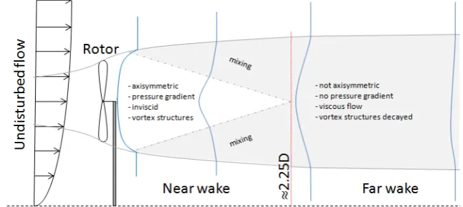
In WAKEFARM wake model, the wind turbine is immersed in the atmospheric boundary layer. The flow field is perturbed by the wind turbine. The flow field is divided into two regions, near-wake and far-wake. The near wake of wind turbine extends approximately 2-3 rotor diameters (D) downstream of the turbine. The near wake region has strong pressure gradients and feels the presence of wind turbine. After near wake, the flow transitions to far wake. In the far wake, turbulence in the atmosphere plays a vital role. The turbulence in the atmosphere reduces the wake deficit and helps in the recovery of wake. The different regions in wake of a wind turbine are shown in Fig 2.1.

In WAKEFARM, the near wake region is modelled using an inviscid vortex method. The effects of turbulence in the atmosphere are added using (parabolized) Navier-Stokes equations together with the kεturbulence model. While simulating multiple

[image:30.595.116.453.411.562.2]

turbines in a row, the output of the first turbine is given as input to the next wind turbine.

Figure 2.1: Different regions in the wake of a wind turbine

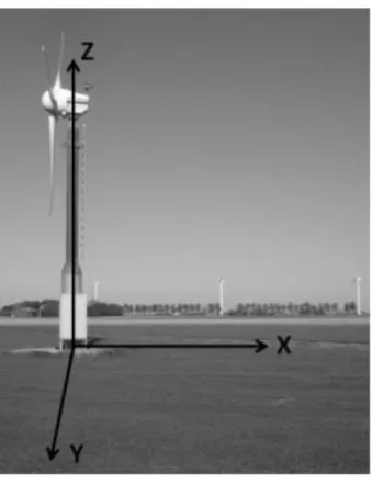
2.1 Coordinate system

WAKEFARM uses cartesian coordinates. The x- coordinate is taken along the wake direction, the y-coordinate is along the span of blade and z- coordinate is in the direction of increasing height.

WAKEFARM has four main components:

(31)

[image:31.595.230.400.90.311.2]

2.2. GOVERNING EQUATIONS 7

Figure 2.2:Coordinate system used in WAKEFARM

• Rotor model

• Free stream model/ Undisturbed flow model

• Near wake model

2.2 Governing equations

In this section, the Governing equations of WAKEFARM are described. WAKEFARM solves steady RANS equations in perturbation form. The RANS equation for turbu-lent flows reads,

∂Ui

∂xi

= 0, (2.1)

∂(UiUj)

∂xj

=−1

ρ ∂p ∂xi

−∂τ

R ij

∂xj

+f, (2.2)

whereτ_ijR is the Reynolds stress, given by. τ_ijR= ∂(U

0

iU

0

j)

∂xj

(2.3)

2.2.1 Perturbed Navier Stokes equations

The mean flowUi is linearized as a sum of undisturbed flow and perturbation. This

(32)

caused by the wind turbine (velocity deficit). The undisturbed flow variables (denoted with subscript ’0’) are obtained from the ABL model described in section 2.4.

U =u0+u νt∗ =νt0+νt k∗ =k0+k, νθ∗ =νθ0+νθ, ε∗ =ε0+ε. (2.4) Parabolizing Navier Stokes equations

The simplification of Navier-Stokes equations by parabolizing the momentum and energy equation is done in most wind farm codes. All the elliptic terms in the stream wise direction are neglected, therefore the Navier Stokes equations in x−direction together with energy equation become parabolic in the axial direction. This means that the information travels only downstream and only information upstream is needed for the calculation. A space marching procedure can be used instead of solving the whole grid [3]. The momentum equations in they−and in thez−direction are elliptic and they have to be solved iteratively in eachx−plane.

Analogy with boundary layer equations

In the boundary layer equatons, the axial pressure gradient is prescribed. It is cal-culated using the flow at the edge of the boundary layer. In WAKEFARM, the the axial pressure gradient calculated from the near wake model (inviscid vortex model) is used as a source term in axial momentum equation. The near wake model is based on inviscid vortex theory. The existing vortex models are discussed in the next chapter 3. The axial pressure gradient thus is not calculated at each spatial step. The assumptions used in the equations are given below [3].

Assumptions

• The flow is steady.

• The flow is incompressible.

• The flow is dominant in the axial direction and there is no flow reversal.

• The velocity in the dominant flow direction is higher compared to the velocity components in other two directions. Hence they are neglected.

• The axial pressure gradient is neglected in the far wake. In near wake, the streamwise pressure gradient is prescribed along with the body force.

(33)

2.2. GOVERNING EQUATIONS 9

• The diffusion in streamwise direction is neglected. ∂τijR

∂xi = 0.

• The turbulent heat conduction in stream-wise direction is neglected.

• The undisturbed flow iny−andz−directions are neglected: v0 = 0,w0 = 0.

• The change in magnitude ofvandwiny−andz−directions are small,The first and second derivatives in two directions can be neglected. ∂2_w

∂y∂z = 0.

Based on experimental observations, Boussinessq proposed that deviatoric Reynolds stress τR

ij is proportional to the mean rate of strain, Now equation for Reynolds

stress,τR

ij can be rewritten in perturbation form as follows,

τ_ijR=ρ(νt0+νt)

∂(ui+ui0)

∂xj

+∂(uj +uj0)

∂xi

− 2

3δij(k+k0), (2.5)

where νt-kinematic turbulent (eddy) viscosity. It is not a material property and

de-pends on flow properties. νt0 is the eddy viscosity associated with undisturbed flow. k, turbulent kinetic energy per unit mass is defined as,

k=

u02+v02+w02

2 (2.6)

k0 is the turbulent kinetic energy present in the undisturbed flow. Expressions 2.37 is used to evaluate the turbulent kinetic energy per unit mass in the undisturbed flow.

u0, v0 , w0 are the turbulent fluctuations in the velocity in the three directions. The

main purpose of velocity fluctuation of turbulence is to enhance the shear stress. The perturbed equations are given by

Continuity: ∂u ∂x + ∂v ∂y + ∂w

∂z = 0 (2.7)

x-momentum equation

(u+u0)

∂u ∂x +v

∂u ∂y +w

∂u ∂z =

∂νt

∂y ∂u

∂y + (νt+νt0) ∂2u ∂y2 +

∂νt

∂z + ∂νt0

∂z ∂u ∂z + ∂νt ∂z ∂u0 ∂z

+ (νt+νt0)

∂2_u

∂z2 +νt

∂u0

∂z +f. (2.8)

the termf inx−momentum equation is the axial pressure gradient calculated from the near wake model. The near wake model is explained in the next chapter.

f =−1

ρ ∂p

(34)

y-momentum equation

(u+u0)

∂v ∂x +v

∂v ∂y +w

∂v

∂z = −

1

ρ ∂p ∂y + 2

∂νt

∂y ∂v

∂y + 2 (νt+νt0) ∂2_v

∂y2 +

∂νt

∂z + ∂νt0

∂z

∂v ∂z

+ (νt+νt0)

∂2_v2

∂z +

∂νt

∂z + ∂νt0

∂z ∂w ∂y − 2 3 ∂

∂y(k+k0),(2.10)

z-momentum equation

(u+u0)

∂w ∂x +v

∂w ∂y +w

∂w

∂z = −

1 ρ ∂p ∂z + ∂νt ∂y ∂w

∂y + (νt+νt0) ∂2w

∂y2 + 2

∂νt

∂z + ∂νt0

∂z

∂w ∂z

+2 (νt+νt0)

∂2_w

∂z2 +

∂νt ∂y ∂w ∂z − 2 3 ∂

∂z (k+k0) +βgθ. (2.11)

A complete derivation of the perturbed Navier-Stokes equations can be found in [3]. Kinematic turbulent viscosity, νt can be expressed as a product of a velocity

scale and a length scale.

νt=Cµvl (2.12)

Two equations (k−ε) are used to model the eddy viscosity term. Usingk andε, the

velocity and length scales are defined as follows,

v =√k (2.13)

l= k 3 2

ε (2.14)

Equations 2.17 and 2.18 are used to predictk andε.

Energy equation

The energy equation is used to model the buoyancy term in the momentum equa-tions. The potential temperature is linearized as a sum of potential temperature of the undisturbed flwo and perturbation.

(u+u0)

∂θ ∂x +v

∂θ ∂y +w

∂θ ∂z =

∂ ∂y

(νθ+νθ0)

∂(θ+θ0)

∂y

+ ∂

∂z

(νθ+νθ0)

∂(θ+θ0)

∂z

(2.15)

which leads to

(u+u0)

∂θ ∂x +v

∂θ ∂y +w

∂θ ∂z =

∂νθ

∂y ∂θ

∂y + (νθ+νθ0)

∂2θ ∂y2 +

∂νθ

∂z + ∂νθ0

∂z

∂θ ∂z

+ (νθ+νθ0)

∂2_θ

∂z2 +

∂νθ0

∂z ∂θ ∂z +νθ0

∂2_θ 0

(35)

2.3. ROTOR MODEL 11

Perturbedk−εturbulence model

The k − ε turbulence is used for the closure of momentum equations. It has 2

equations [22, 23, 24],

• Equation for turbulent kinetic energy per unit mass-k

• Equation for the rate of dissipation of turbulent kinetic energy per unit massε

Equation 2.17 calculates the energy in turbulence and Equation 2.18 calculates the scale of turbulence. Turbulent kinetic energy:

(u+u0)

∂k ∂x+v

∂k ∂y+w

∂(k0+k)

∂z = (νk+νk0)

∂2_k

∂y2+(νk+νk0)

∂2_k

∂z2+

∂νk

∂y ∂k ∂y+(νk)

∂2_k 0

∂z2

+ (νt+νt0) " ∂u ∂y 2 + ∂u ∂z 2

+ 2∂u

∂z ∂u0

∂z

#

+νt

∂u0

∂z

2

−βgνθ

∂θ ∂z + ∂θ0 ∂z

−βgνθ

∂θ ∂z

(2.17) Dissipation rate of the turbulent kinetic energy:

(u+u0)

∂ε ∂x+v

∂ε ∂y+w

∂(ε0+ε)

∂z = (νε+νε0)

∂2ε

∂y2+ (νk+νk0)

∂2ε ∂z2 +

∂νε

∂y ∂ε

∂y+ (νε) ∂2ε0

∂z2

+

∂νε

∂z + ∂νε0

∂z ∂ε ∂z+ ∂νε ∂z ∂ε0

∂z +νε ∂2ε0

∂z2 +Cε1

ε0+ε

k0+k

(νt+νt0)

" ∂u ∂y 2 + ∂u ∂z 2 + ∂u0 ∂y 2# +2∂u ∂z ∂u0

∂z + (1−Cε3)βg 1

σθ

∂(θ+θ0)

∂z +Cε1 ε0

k0

νt0

"

∂u0

∂z

2

−(1−Cε3)βg

1

σθ

∂θ0

∂z

#

−Cε2

(ε0+ε)2

k0+k

+Cε2

ε2 0

k0

(2.18)

The closure coefficients are,

Cµ= 0.033, C1 = 1.21, C2 = 1.92, C3 = 0.8, σθ =σk = 1.0, σ= 1.3 (2.19)

2.3 Rotor model

(36)

U∞, far downstream isUe, and at the rotor disc, it is taken asUR. The velocity at the

rotor according to actuator disk momentum theory is defined as follows,

UR=

1

2(U∞+Ue) (2.20)

2.3.1 Induction factor and thrust coefficient

A non-dimensional quantity called induction factor is defined as follows,

a= U∞−UR

U∞

(2.21)

The velocity at the rotor disc and far downstream is defined as follows,

UR =U∞(1−a) (2.22)

Ue=U∞(1−2a) (2.23)

The thrust coefficient is defines as follows,

CT =

T

1 2ρU∞2

= 4a(1−a) (2.24)

For heavily loaded rotors, Glauert included a correction. The Glauert correction

Figure 2.3: Pressure and Velocity distributions in actuator disk model

reads as follows,

φm =

         1 2 1−

√

1−0.8, ifa >1.4

1

2(−2.5(CT −0.8) 2₊_C

T + 0.2−

√

1−0.8), if0.8< a <1.4

1 2 1−

√

1−CT

, if0< a <0.8

(37)

2.4. UNDISTURBED FLOW MODEL- ATMOSPHERIC BOUNDARY LAYER STABILITY MODEL 13

2.4 Undisturbed flow model - Atmospheric boundary

layer stability model

The undisturbed flow here is referred to as the flow far upstream of the wind turbine. This mainly consists of the atmospheric boundary layer (ABL) above the surface of earth. The Atmospheric boundary layer in WAKEFARM is modelled using two different empirical models suggested by Panofsky-Dutton [25] and Gryning[26].

2.4.1 Panofsky Dutton ABL model

Panofsky model uses a surface layer model to model the atmospheric boundary layer. The surface layer is the lower 10% part of the atmospheric boundary layer,

where the magnitude of wind speed changes. The direction of wind is more or less constant.

Velocity profile

The undisturbed mean flow0_u0

o and turbulent statistics is to be modelled. The

undis-turbed flow is assumed to vary in z-direction only. The Reynolds number in the stream-wise direction is very high, hence stream-wise diffusion is neglected. The molecular viscous stresses are small compared to the Reynolds stress term u0w0.

By Boussinessq approximation the Reynolds stress is defined as follows,

τR=u0w0 =ρνt0

∂u0

∂z (2.26)

whereνt0is eddy viscosity or turbulent viscosity,u0undisturbed mean flow,u∗friction

velocity, the characteristic velocity at the wall is expressed as follows[25]

u∗ = s

τR

ρ (2.27)

leading to

∂u0

∂z = u2

∗

νt0

(2.28)

Monin and Obukhov in their similarity theory [27] calculated eddy viscosity νt0 as follows,

νt0 =

ku∗z

φm(_Lz)

(2.29)

where von Karman constant,k, taken as 0.4 in [18],φm Monin Obukhov function, L

(38)

2.29,

∂u0

∂z = u∗

kzφm

z L

(2.30)

Both sides of equation (2.30) are integrated fromz0 toz, to obtain the velocity profile.

Z z

z0

∂u0

∂z dz =

Z z

z0

u∗

kzφm

z L

dz = u∗

k Z z z0 1−

1−φm

z L dz z (2.31) leading to,

u0(z) =

u∗ k ln z z0

−Ψm(ξ)

(2.32)

whereξ=_Lz, together with,

Ψm(ξ) =

Z ξ

0

(1−φm(ξ))

dξ

ξ (2.33)

Ψm is stability correction function discussed in C.3. The value of the function varies

as the stability of the atmosphere varies (see section C.0.1) to learn about stability classification.

Potential temperature profile

Similar to the velocity profile, potential temperature profile can be derived

θ0−θ0s =

T∗ k ln z z0

−Ψh(ξ)

, (2.34)

Ψh(ξ) =

Z ξ

0

1− νθ0

νt0

φm(ξ))

dξ

ξ (2.35)

where,

T∗ =

Q ρCpu∗

(2.36)

with, νθ0 is the thermal diffusivity of heat, θ0s is the potential temperature of the

ground,Q is the turbulent heat flux to the ground. Ψh is stability correction function

discussed in section C.3.

Profile of k0 and0

The expression for the profile of turbulent kinetic energy in ambient flow as given in [18], is as follows

k0(z) =

u2

∗ p

Cµ

(39)

2.4. UNDISTURBED FLOW MODEL- ATMOSPHERIC BOUNDARY LAYER STABILITY MODEL 15

where Cµ is a constant used in k −ε model and is set as 0.033. Similarly the

expression for dissipation rate of turbulent kinetic energy in ambient flowε0 used in WAKEFARM is given below,

ε0(z) =

3u∗

kz Ψe(ξ) (2.38)

Ψe(ξ)andΨk(ξ)are stability correction functions discussed in section C.3

2.4.2 Gryning ABL model

Gryning [1] mentions that the height of surface layer is in the order of50−80m. The

wind turbines have grown in size. Haliade-X which is the world’s powerful offshore wind turbine to date (July 2018), has a total height of260m. The upper part of wind

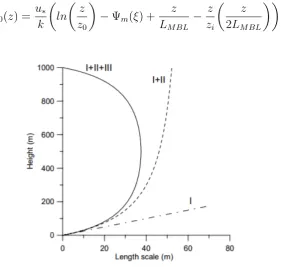
turbine lies outside the surface layer[28]. Sathe et.al. [28] showed that by using the surface layer profile in higher heights, the loads are predicted much larger compared with those obtained using a boundary layer wind profile (which includes an accurate description of above surface layer profiles) [28]. Hence the assumption that the whole of wind turbine lies in the surface layer is not reliable. The wind profile length

lscale consists of 3 terms, surface layer length scaleLSL, length scale in the middle

of boundary layerLM BL, length scale in the upper boundary layerLU BL.

1

l =

1

LSL

+ 1

LM BL

+ 1

LU BL

(2.39)

Figure 2.4 illustrates the behaviour of the 3 length scales for a neutral boundary layer of height1000m. The surface layer where the length scale varies linearly with height

is applicable only up to 50m. After 50m, the influence of LM BL can be seen. The

height of the boundary layerLU BLinfluences the length scale at150m. The different

types of atmospheric stability are discussed in section C.0.1.

Velocity profile

A detailed derivation of velocity profile is given in [26]. The velocity profile is given by,

Neutral conditions

u0(z) =

u∗ k ln z z0 + z

LM BL

− z

zi

z

2LM BL

(40)

Stable conditions

The profile ofu0 for stable conditions reads[1],

u0(z) =

u∗ k ln z z0 + 5z

L

1− z

2zi

+ z

LM BL

− z

zi

z

2LM BL

(2.41)

Unstable conditions

For unstable atmospheric conditions, the undisturbed wind profile can be expressed as,

u0(z) =

u∗ k ln z z0

−Ψm(ξ) +

z LM BL

− z

zi

z

2LM BL

[image:40.595.138.425.247.514.2]

(2.42)

Figure 2.4: Profiles of the length scale for neutral conditions with boundary layer height of 1000m and roughness length z0 = 0.05m The dashed-dotted line correlates to the surface layer scaling. The dashed line includes the effect of first two terms and the full line includes the effect of all three terms in the formulation of the length scale [1].

The stability correction function Ψm(ξ) is obtained from equation C.9. In all the

equations above, Lrepresents the Monin-Obukhov length,LM BL, the length of

mid-dle boundary layer zi, the total height of the boundary layer,u∗, the friction velocity

near the ground surface, z, vertical position

(41)

2.5. GRID GENERATION 17

Table 2.1: Stability classification based on Monin-Obukhov length(L)

10< L < 50 Very Stable 50< L <200 Stable 200< L < 500 near neutral/stable

L >500, L < −500 neutral

−500< L < −200 near neutral/unstable

−200< L < −100 unstable 100< L <−50 very unstable

Parameterization ofLM BL

The length of middle boundary layer LM BL is calculated from the following

expres-sion

u∗

f LM BL

=

−2ln

u∗

f z0

+ 55 exp − u∗ f L 2 400 (2.43)

The above expression is derived by relating the wind speed at the top of the bound-ary layer to the friction velocity u∗ near the ground [1]. By knowing u∗, L, z0 and Coriolis forcef, LM BL can be derived. The height of the boundary layer is

approxi-mated as

zi ≡0.1

u∗

f (2.44)

The profile of potential temperatureθ0,k0,ε0 are calculated with expressions in sec-tion 2.4.1. The stability classificasec-tion is given in the table 2.1 [1].

2.5 Grid generation

WAKEFARM uses a stretched grid in thex−direction and an uniform grid iny−and

z−directions. The grid is stretched until0.5D, and from then on the grid is uniform. A

finer grid is used close to the rotor, where sharp gradients are present. The domain extends to7.5Dinx−direction,3.8Diny−andz−directions.

2.6 Numerical methods

(42)

[image:42.595.175.393.85.310.2]

Figure 2.5: Computational domain iny−z plane in WAKEFARM [2]

calculate the pressure gradients in y and z directions. (see section 2.6.2) and ADI

method (Alternating Direction Implicit scheme (section 2.6.1)). The idea behind us-ing ADI methods is to obtain a tridiagonal system which is easier to solve. In ADI method, computational domain is swept one line at a time. To obtain a tridiagonal system, the governing equations in WAKEFARM equations 2.8 -2.18 are rewritten in a new way. The elements outside three diagonals are moved to the right-hand side of the equation. Their values are assumed to be known. The process is repeated till convergence [29] In a row-wise sweep, the information propagates instantaneously from left to right boundary. However, the information does not propagate efficiently in the other direction. To circumvent this checkerboard problem, the direction of the line wise sweeps is alternated. Hence the name alternating direct implicit method [29]. The resulting tridiagonal system is solved by using Thomas algorithm. While solving the momentum equations in an iterative way, non-uniform pressure field or oscillatory pressure fields may occur in the intermediate steps. Central differences might not be able to capture such a non uniform pressure field. Upwind schemes could be used, but they have a disadvantage that the information travels only from one direction. To avoid these issues, a staggered grid is used for pressure (see Figure 2.7) [3]. The velocities are calculated in the main grid points (solid points in Figure2.7) and the pressure is calculated in the staggered grid points (crosses in Figure2.7). While deriving the pressure correction formula for the SIMPLE algo-rithm, the continuity equation is written on the staggered grid. The derivation of the pressure correction formula can be seen in [3].

(43)

2.6. NUMERICAL METHODS 19

terms are modelled by central differences.

2.6.1 ADI method

The variable Φi,j denotes the flow variables in WAKEFARM (u, v, w, p, t, k, ε). All

the 7 governing equations in WAKEFARM are solved using ADI method. The ADI

method is summarized below.

• Start with an initial guessΦi,j

• Set up a tridiagonal solver for each row (e.g. row wise sweep). This can be treated as an intermediate step (step atn+1₂).

• Set up a tridiagonal solver for each column (e.g.column-wise sweep). The updated solution from the row wise sweep is used as an initial guess to the column-wise sweep (n+1 step).

• Iterate till convergence

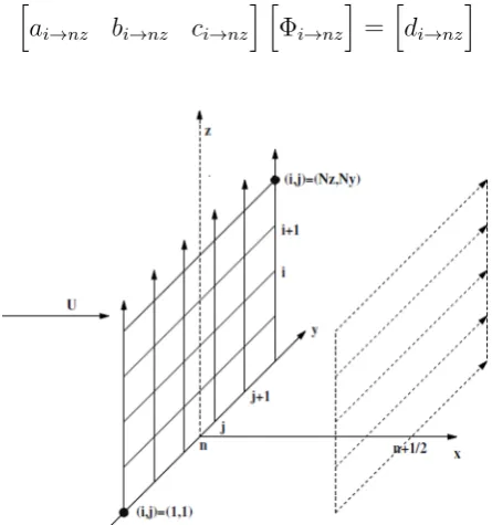
aiΦi+1,j+biΦi,j+cj−1,i=d (2.45)

where, d is the known value (value at the current iteration) of the entries outside the tridiagonal system. The following set of equations are obtained.

h

ai→nz bi→nz ci→nz

i h Φi→nz

i

=hdi→nz

i

[image:43.595.201.424.472.710.2]

(2.46)

(44)

2.6.2 The SIMPLE method

The SIMPLE algorithm is summarized below,

• Calculate the velocity field for the next axial plane from the momentum equa-tions using ADI method.

• Obtain pressure correction from the pressure correction formula.

• Perform Gauss Seidel relaxation, till the continuity equation is satisfied.

• Once the pressure is converged, the velocities are calculated fromy−momentum andz−momentum equations.

• When the above mentioned steps are completed, the values of θ, k, ε are

calculated for the next axial plane, using ADI method.

• Complete the space marching procedure.

A detailed description of the SIMPLE method is found in [30]

Figure 2.7: Staggered grid

(45)

2.7. EXAMPLEWAKEFARM RESULT 21

2.6.3 Boundary conditions

The boundary conditions are specified at the extremities of each y−z plane (see

Figure 2.6) at each spatial step. On all the boundaries, the flow reaches frees stream conditions (u0,v0,w0. The perturbation values at the boundaries should be zero :

u=v =w=p=θ=k =ε = 0 (2.47)

substituting this in they−momentum equation we get, −1

ρ ∂p

∂y ≈0 (2.48)

The same exercise can be repeated to top and bottom edge of the domain using

z− momentum equation. The pressure at the first row of points inside normal grid should be zero. The boundary condition for pressure reads,

p_j₋1 2,i−

1

2 = 0f or 





j = 1,2, N y, N y+ 1, i= 1,2, ...., N z+ 1

i= 1,2, N z, N z+ 1, j = 1,2, ....N y+ 1 (2.49)

2.7 Example WAKEFARM result

The horizontal velocity profile in the cross-flow direction at hub height and at down-stream distance 2.5D is presented in this section. The velocity profile measured

in EWTW measurements show a higher velocity deficit compared to velocity deficit predicted by WAKEFARM (see Figure 2.9). Towards the centre of the wake, the ex-perimental velocity profile shows a small hump. This is due to the presence of root vortex in the wind turbine wake. This behaviour is not captured by WAKEFARM. The centerline velocity profile at a downstream distance of5D is also presented in

(46)

Figure 2.9: Comparison of horizontal velocity profile in the cross flow direction at hub height and at downstream distance 2.5D with EWTW

measure-ments. The axial induction factor at rotora = 0.245and the free stream

velocity at hub height is11m/s

Figure 2.10: Comparison of centerline velocity profile at downstream distance of

x−5D with Marchwood experimental data. The thrust coefficient at

(47)

Chapter 3

Inviscid near wake model

improvement

In chapter 2 it was mentioned that, in the axial momentum equation, pressure gra-dient was not calculated iteratively. The axial pressure gragra-dient in far wake is ne-glected, as it is negligible. Earlier the near wake was not included in the numerical simulation of the fluid flow equations. The velocity profile in near wake was repre-sented by a gaussian shaped velocity profile. The space marching was started at downstream position 2.25D. Later to reduce the dependency on tuning parameters and to model the wake in a realistic way, the wake of wind turbine was modelled using inviscid vortex methods. The pressure field is calculated using Bernoulli’s equation. The pressure gradients are then calculated numerically using finite dif-ferences. The calculated axial pressure gradient is prescribed along with the body force. The induced velocities calculated in three directions are given as an initial guess to the perturbation in perturbed Navier Stokes equations (2.8-2.11). The existing vortex models used in WAKEFARM are discussed initially and later, the improvements made are discussed in detail.

3.1 Existing inviscid vortex model

3.1.1 Vortex tube model

In this model, the wind turbine is approximated as actuator disk, the wake is repre-sented as vortex tube (see Figure 3.1). The vortex rings are discretized as straight vortex filaments. The method is free-wake method, where the wake radius is a part of the solution process. The boundary condition given is that there is no pressure jump across the tube. The free-wake method is computationally expensive. But since the flow in the wake and the resulting axial pressure gradient is only a func-tion of the inducfunc-tion factor, for a set of inducfunc-tion factors the resulting velocity profile

(48)

scaled with rotor diameter is stored a priori in a database [4]. This database is known as ’Tube files’.

Figure 3.1: Wake represented as a vortex tube [4]

3.1.2 Oye’s vortex ring model

Apart from the vortex-tube near wake model, another near-wake model exists in WAKEFARM. It is based on vortex ring model suggested by Oye [5]. Oye ’s vortex model assumes wind turbine as an actuator disk (a rotor with infinite number of blades). The actuator disk has a constant loading throughout the disk and hence infinitely thin vortex rings are trailed from the edges of the disk. They describe the wake. The vortex ring wake structure expands behind the turbine forming a vortex tube of increasing radius as shown in figure 3.2. The vortex densities on the surface of the tube are resolved into axial and tangential components, as seen in Figure 3.3. The model also assumes infinite tip speed ratios, the hub radius to be zero and hence root vortex and the induced velocity contribution from the axial component of vortex density can be ignored. The velocities induced in axial and radial directions are produced by the tangential component of vortex density (see Figure 3.3). The tangential component of vortex densityγt, is defined as follows [5],

γt=Ct

U2

∞ 2Va

(3.1)

where U∞ is undisturbed free stream velocity at hub height, Va, velocity induced

by tip vortices in axial direction and Ct, thrust coefficient at the rotor. Equation 3.1

is used to calculate the tangential vortex density γt at each iteration. A complete

derivation of equation 3.1 is found in [5].

The wake is modelled by using discrete vortex rings. Each vortex ring repre-sents a wake segment of length dx (see Figure 3.2). The vortex rings are placed

in the middle of wake segment and at a distance equal to local wake radius in the

(49)

3.1. EXISTING INVISCID VORTEX MODEL 25

Figure 3.2: Model of wind turbine wake with discrete ring vortices

Figure 3.3: Resolving the vortex density on the surface of a single tip vortex into its axial and tangential components[5].

each vortex ring can be calculated from the analytical expression for velocity induced by a vortex ring (see equation A.1 and equation A.2). The elliptic integrals are eval-uated numerically. As the vortex strength and axial induced velocity are interrelated, the system is non-linear. The wake radius is calculated from the continuity equation for axial flow, i.e. the total flow through each section of the wake is same as the flow through the rotor disc. The axial velocity at 0.7R is calculated at the rotor and at

several downstream positions in the wake. It is assumed to be a good estimate to the average axial velocity at each cross-section in the wake. The continuity equation for axial flow is written as follows

ρArotorV0.7(0) =ρAwakeV0.7(xi) (3.2)

After further simplifications the following equation for wake radiusri is obtained

ri =R

s

V0.7(0)

V0.7(xi)

(50)

with Arotor is the area of the rotor,Awake is the cross sectional area at the selected

downstream position,V0.7(0)is the axial velocity at0.7Rin the rotor plane,V0.7(xi)is

the axial velocity at 0.7R and downstream positionxi. The methodology is

summa-rized below.

1. Iteration starts with an initial guess of tangential vortex density γt(i) for each vortex ring. Equation 3.1 is used for the calculation. The strength of the vortex ring is calculated as follows,

Γi =

1

2γt(i)+γt(i−1)

dx (3.4)

2. The axial induced velocity is initially guessed to be free stream velocity and the wake radius to be rotor radius (r)

3. Axial induced velocitieswxfor the vortex ring strengthΓiare calculated at three

different locations, small distancedy outside the vortex ring, small distancedy

inside the vortex ring, and at0.7ri (positions marked by crosses in Figure 3.2).

4. Axial velocity at wake surface is taken as the average of axial velocities at small distancedyto both sides of the surface (crosses in positions outside and

inside the wake in Figure 3.2)

Va =U∞+ 1

2(wx(r+dy) +wx(r−dy)) (3.5)

5. The new estimate for the tangential vortex density γt(i) is calculated with the newly calculated axial induced velocityVa using expression 3.1

6. The wake radius is calculated by the equation of continuity for axial flow (equa-tion 3.3).

7. The process is repeated till the wake radius is converged.

With the calculated vortex densitiesγt(i), the axial and radial induced velocities at all grid points are calculated using formulae A.1 and A.2. A singularity results when the control points approach the vortex ring. To circumvent this issue, a linear profile is assumed near the vortex core. Total induced velocity at each evaluation point can be calculated by adding up the induced velocity contribution from each vortex ring. The total induced velocities inx−, y−andz−directions at a point are calculated by adding up the velocity contributions from N−vortex rings, as follows

Va= N

X

i=1

(51)

3.2. PURPOSE OF IMPROVING THE VORTEX MODELS 27

Vy =cos tan

z−H y

!! _N X

i=1

wy(r, θ, x) (3.7)

Vz =sin tan

z−H y

!! _N X

i=1

wy(r, θ, x) (3.8)

To reduce the computational time, domain is split into two equal parts, withx−z

plane as symmetry plane. The results are mirrored along thex−z plane.

Pressure Gradients

The pressure in the wake can be calculated from Bernoulli’s equation. Pressure at any evaluation point,p2 is calculated using velocityu2, free stream velocity u∞ and

ambient pressurep∞as follows,

p∞+ 1 2ρu

2

∞ =p2+

1 2ρu

2

2 (3.9)

with,p∞ is ambient pressure, u∞, free stream velocity. The pressure gradients in 3

directions, ∂p ∂x,

∂p ∂y and

∂p

∂z are calculated from pressure using finite differences. The

perturbation variablesu, v,win the perturbed Parabolized Navier Stokes equations

are initialized using the near wake model. The induced velocities Va, Vy and Vz are

given as an initial guess to the perturbation variables.

3.2 Purpose of improving the vortex models

There is a discrepancy between the WAKEFARM results and experimental data (see Figure2.10, Figure 2.9). The experiments show a higher velocity deficit compared to velocity deficit predicted by WAKEFARM. Towards the centre of the wake, the experimental velocity profile shows a flattened behaviour. This discrepancy might be the result of using a relatively simple vortex ring model to model the wake of wind turbine and ignoring the root vortex while modelling the wake of wind turbine

• Need for radially varying circulation model: The existing models in WAKE-FARM assume a uniform loading along the actuator disk, hence the vorticity is trailed only at the edges. Such a model of a wind turbine is hypothetical. In a real wind turbine, the bound circulation varies along its span, as the bound circulation has to vanish continuously at the blade extremities. Hence a model of wind turbine with radially varying circulation is needed.

(52)

typically modelled as a single axial vortex not influencing the axial component of velocity[31]. Real wind turbines do have a root section and a rotor hub, to which all the blades are attached. The energy is not extracted in the hub and root sections of the wind turbine, hence their presence does have an impact on the axial velocity profile. The root vortex too plays an important role in the evolution of wake closer to the turbine, the near wake and hence on the wake far downstream of the turbine, known as far wake (see Figure 2.1) [12, 31]. Thus modelling the flow near the root section is essential.

• Need for a helical wake model: At extremely high tip speed ratios, the pitch of the helix becomes extremely small and the spirals of the helix come closer to each other (see Figure 3.4). In such conditions, the helical tip vortices can be approximated as circular vortex rings. The assumption is erroneous when the tip speed ratios are small. Apart from that, helical fragments with shorter radius cannot be approximated as vortex rings even at higher tip speed ratios (see Figure 3.4). To include the effect of finite tip speed ratios and finite number of blades, a helical model of the wake is necessary.

Figure 3.4: Side view of trailing helices, for different tip speed ratios.λ = 6(left),λ = 9(right)

(53)

3.3. DEVELOPMENT OF VARYING CIRCULATION,CONSTANT AXIAL INDUCTION MODEL 29

3.3 Development of varying circulation, constant

ax-ial induction model

3.4 Span varying bound circulation

Joukowsky defined an ideal rotor as the one with constant circulation along its span [32]. The Joukowsky rotor has an uniform loading, hence a constant bound cir-culation along the blades. However in reality wind turbine rotors have a varying circulation along the blade span. For a real flow, the bound circulation varies along the span, because the circulation has to vanish continuously at the blade extrem-ities. As a result of this, the strength of the vortex sheets increases towards the blade extremities [12]. Due to this varying bound circulationΓb(r), vorticity is trailed

from different sections along the blade. When the circulation is not constant along the blade, each blade sheds a helical vortex sheet from its trailing edge. The ax-ial component of helical sheet induces tangentax-ial velocity in anti-clockwise direction (opposite to the direction of rotation of rotor). The azimuthal component of helical sheet induces an axial velocity in the upstream direction [12]. The helical sheet of vorticity undergoes expansion and distortion. As a starting point, wake expansion and distortion are ignored.