Preference learning: What defines an optimal shift schedule?

(1)

December 2, 2019

PREFERENCE LEARNING

WHAT DEFINES AN OPTIMAL SHIFT

SCHEDULE?

Sanne van Weersel Master thesis

Supervisors university Company supervisor

dr. ir. W.J.A. van Heeswijk L.M. Fijn van Draat, MSc dr. ir. J.M.J. Schutten

University of Twente ORTEC

(2)

(3)

Management summary

Problem description

This research studies the problem of creating shift schedules. Since shift schedules are sub-jected to many strictly regulated rules, shift scheduling is considered to be a complex problem. Moreover, nowadays, preferences of employees are getting more and more important.

For this, ORTEC provides an optimization algorithm that creates shift schedules: the Opti-mizer. Using the Optimizer to create shift schedules brings several advantages, among others, time savings for the planners and an increased resource efficiency.

In the Optimizer rules are regulated as hard constraints and preferences assoft constraints. Practice has shown that translating scheduling preferences into soft constraints for the Optimizer is challenging and time consuming for the following reasons: i) It is hard to articulate preferences, ii) Preferences are company specific and iii) Preferences change over time. As a consequence, a vast amount of the current customers creates shift schedule manually and does not use the Optimizer.

Planners perceive these manually created shift schedules as desirable. Therefore, we expect that historical shift schedules contain valuable information that can be used to identify scheduling preferences of customers. The objective of this research is to explore how ORTEC can use these historical shift schedules to identify scheduling preferences and formulate soft constraints for the Optimizer.

Approach

This thesis focuses on identifying scheduling preferences for departments within an organization. Based on three customer cases, we formulate four categories of soft constraints:

• Consecutive duties: these constraints define if scheduling two duties on succeeding days is desirable, undesirable or indifferent.

• Free weekends: the preferred number of free weekends an employee should have per period. In this constraint, the customer is also required to define the length of the period in weeks for which the constraint holds.

(4)

• Distribution of weekend shifts: This category contains two types of soft constraints: i) The preferred minimum and maximum series length of night shifts and ii) The frequency that employees should work night shifts.

For each of the types of soft constraints, we use both domain knowledge (e.g. information such as employee skills, demand for shifts, known preferences and labor laws) and the historical shift schedule to identify the preferences of the customer. Using domain knowledge helps us to structure the soft constraints and prevents us from suggesting irrelevant constraints. Thereafter, data mining techniques (e.g. cluster analysis and association rule mining) identify frequent patterns in the historical shift schedule of customers. These frequent patterns represent the scheduling preferences of the customers.

Results

For each of the categories of soft constraints, applying the method we propose gives the following insights:

• Consecutive duties: The algorithm detects 40% to 100% of the most important desirable and undesirable combinations of consecutive duties. Not all combinations detected by the algorithm are indeed a preference of the customer. Domain knowledge removes irrelevant combinations of duties and thereby improves the performance of the algorithm. In practice, the consultant and planner should verify whether all identified combinations of desirable and undesirable duties are relevant and if any imported combinations are missing.

• Free weekends: The algorithm is able to identify the preferred number of free weekends with a small error. However, the algorithm did not succeed in identifying the length of the period the constraint holds for. Domain knowledge ensures that the correct employees are included in the analysis and increases the performance of the algorithm. In practice, the consultants can trust the number of free weekends identified by the algorithm. However, the consultants should verify with the planner for which period the constraint holds.

• Preferred series length: The algorithm could identify the range of series length that oc-curred frequently in the past per type of contract. In most customer cases, this range was in line with the preferences of the customers. The algorithm detects frequent series lengths in the historical data, however, it did not succeed in identifying if the preference exists or not for all types of contracts. Therefore, in practice, consultants should verify with the planner if the preference exists or not.

(5)

Conclusions

The method we propose gives insights in which events occurred frequently in the past. In this research, most customers perceived these frequent patterns as preferred and we could identify the preferences with only a small error.

(6)

Acknowledgments

With this thesis, I finish my master Industrial Engineering and Management and with that my time as a student at the University of Twente comes to an end. The past years have been a great time of learning new things and building strong friendships.

I would like to express my appreciation to ORTEC for giving me the opportunity to write this master thesis. In particular, I would like to thank Laurens Fijn van Draat for sharing his knowledge, having a critical look during the whole process and challenging me to achieve the best results. Additionally, I would like to thank Egbert van der Veen for the monthly brainstorm sessions, this really helped me in choosing the right direction of the research. Finally, I would like to thank my colleagues from OWS for making it a great work place, both working as a graduate intern and as a student assistant.

Furthermore, my acknowledgments go to Wouter van Heeswijk and Marco Schutten, my su-pervisors of the University of Twente, for providing useful feedback, giving valuable insights and being good discussion partners. Without their support, the whole process would have been much more complicated.

(7)

Abbreviations

CLA Collective Labor Agreement.

GA Genetic Algorithm. GI Greedy Insertion.

IQR Interquartile Range.

MAE Mean Absolute Error. MSE Mean Squared Error.

NSP Nurse Scheduling Problem.

OWS ORTEC Workforce Scheduling.

RMSE Root Mean Squared Error.

SS Sum of Squares.

(10)

Chapter 1

Introduction

This research takes place at ORTEC in Zoetermeer. ORTEC provides software solutions to improve their customers’ decision-making processes and operations. ORTEC provides these soft-ware solutions for different business processes, such as workforce scheduling, routing, loading, warehousing and field services. One of the products ORTEC provides is ORTEC Workforce Scheduling (OWS), which supports organizations with their shift scheduling. This chapter pro-vides an introduction to this research. Section 1.1 describes the shift scheduling problem in general, followed by a description of the functionalities of OWS. Section 1.2 introduces the prob-lem to tackle, followed by the objective of this research in Section 1.3. Section 1.4 describes the research framework.

1.1 Problem background

The shift scheduling problem is a well-studied problem and several approaches exist in the lit-erature to solve this problem. This section provides a short description of existing approaches to solve the shift scheduling problem in Section 1.1.1. Section 1.1.2 provides an introduction of ORTEC’s software solution for shift scheduling: OWS.

1.1.1 Shift scheduling

In the past few decades, shift scheduling has been heavily investigated within the fields of oper-ations research and artificial intelligence (Van Den Bergh et al., 2013). According to Van Den Bergh et al. (2013), this increased research attention could be motivated by economic consider-ations of organizconsider-ations. For many organizconsider-ations, their workforce is one of their most valuable assets but also a major direct cost (Van Den Bergh et al., 2013). In other words, reducing the costs by a small percentage could already be very beneficial (El Adoly et al., 2018).

Shift schedules are subjected to many strictly regulated rules and company-specific rules. Consequently, the shift scheduling problem is to be considered as a complex process. An exam-ple of such a rule is the following Working Hours Act (WHA) rule: ’If a night shift ends after 2 am, this must be followed by a minimum of 14 hours of non-work time. This may be shortened

to 8 hours a maximum of once per week. But only if the type of work or the business

(11)

employees may have preferences for the shift schedule; for example, the preference to work at a specific location. Nowadays, it is getting more important for companies to satisfy employees, therefore, personal preferences are considered as well while creating a shift schedule (Van Den Bergh et al., 2013). Similarly, organizations have preferences while scheduling shifts; for example, assigning unpopular shifts fairly. For planners, it is hard to come up with a shift schedule that respects all labor laws and preferably satisfies the employees’ and the organization’s preferences (Brooks and Swailes, 2002). In the literature several approaches to solve the shift scheduling problem considering both labor laws and scheduling preferences exist; some of these approaches are:

i Nurse Scheduling Problem

Within operations research, the shift scheduling problem is also known as the Nurse Scheduling Problem (NSP). In the NSP, regulations and labor laws are modeled as hard constraints. To be considered feasible, a solution must satisfy all these hard constraints. Scheduling preferences are modeled as soft constraints. Satisfying these soft constraints increases the quality of a schedule, however, violation of a soft constraint can still lead to a feasible shift schedule (Bl¨ochliger, 2004). Each soft constraint has an associated weight

expressing its relative importance. The objective function of the optimization problem is two-fold. One part of the objective function minimizes the workforce costs incurred with a shift schedule. The other part represents to what extent the shift schedule satisfies the scheduling preferences, which is a combination between the weights and extent to which soft constraints are violated (Smet et al., 2013). Several methods exist to solve the NSP, for example, by using a linear programming model (Jaumard et al., 1998). The NSP is known to be an NP-hard problem (Solos et al., 2013). Consequently, small scheduling problems can be solved optimally, while complex scheduling problems are often solved by using a combination of heuristics (Brucker et al., 2011).

ii Self-rostering

Another approach to solve the shift scheduling problem is self-rostering. With self-rostering, employees propose a preferred shift schedule for the scheduling period (Van der Veen et al., 2016). In this way, self-rostering copes with the personal preferences of employees. In order to satisfy all hard constraints, the proposed shift schedules must comply with labor laws and the employee’s contract hours. When the proposed schedules do not match the demand for shifts as defined by the organizations, shifts need to be reassigned. Reassigning these shifts can be solved by using an iterative improvement heuristic (Van der Veen et al., 2016). A drawback of self-rostering is that it only works under certain circumstances; a certain level of collegiality is required and the department should not be too large (Drouin and Potter, 2005). Moreover, Silvestro and Silvestro (2000) show that using a self-rostering system is difficult in departments that include more than 35 employees.

iii Preference rostering

(12)

while satisfying all hard constraints. To be implemented successfully, the department size should not be too large and a certain level of collegiality should exist.

1.1.2 ORTEC Workforce scheduling

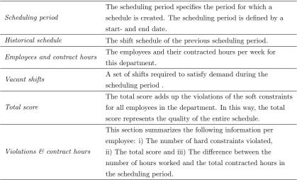
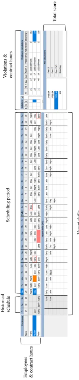
[image:12.595.89.509.259.513.2]

ORTEC provides a software solution, OWS, that supports organizations with creating shift schedules. In general, organizations are divided into different departments. For each department 1_{, the shift schedule is represented in a planning board as shown in Figure 1.1. The planning} board displays all information needed to create a shift schedule for a given scheduling period. Table 1.1 describes the terminology used in the OWS planning board.

Table 1.1: Terminology OWS planning board

Scheduling period

The scheduling period specifies the period for which a schedule is created. The scheduling period is defined by a start- and end date.

Historical schedule The shift schedule of the previous scheduling period.

Employees and contract hours The employees and their contracted hours per week for

this department.

Vacant shifts A set of shifts required to satisfy demand during the

scheduling period .

Total score

The total score adds up the violations of the soft constraints for all employees in the department. In this way, the total score represents the quality of the entire schedule.

Violations & contract hours

This section summarizes the following information per employee: i) The number of hard constraints violated, ii) The total score and iii) The difference between the number of hours worked and the total contracted hours in the scheduling period.

Planners can use OWS for manual-scheduling by assigning a vacant shift to one of the available employees. OWS supports the planner to cope with the high number of hard and soft constraints by highlighting violations and presenting the total score of the schedule. In addition, OWS has a feature to automatically create shift schedules for a department. Within OWS, this feature is known as the Optimizer. In short, the Optimizer assigns vacant shifts to the employees, resulting in a shift schedule.

In the Optimizer, the scheduling problem is formulated as an NSP. In order to use the Opti-mizer, all regulations and preferences must be explicitly modeled as a hard or a soft constraint. Figures 1.2 and 1.3 show an example of one of the hard and soft constraints, respectively. The white input fields allow the customer to change the parameters of a constraint. In contrast to hard constraints, soft constraints require a weight between 1 and 10,000, which reflects its rela-tive importance. Currently, OWS contains around 110 types of hard constraints and 40 types of soft constraints. In order to use the Optimizer, customers select a set of relevant hard and soft

1_{In practice, a department is often split up into several scheduling groups. In this research we refer to a}

(13)

[image:13.595.231.359.109.723.2]

(14)

constraints that represent their scheduling problem. Subsequently, each of these hard and soft constraint can be customized by changing its parameters and, if needed, its weight.

The scheduling problems of ORTEC’s customers are often complex problems; shift schedules for large departments must be created considering a large number of constraints. For one of the customers, every week 1952 shifts have to be scheduled in a department including 139 employees. Due to the complexity of these scheduling problems, the Optimizer uses a combination of several heuristics to solve this optimization problem within a reasonable time. Chapter 2 provides a detailed description of the heuristics used in the Optimizer.

Figure 1.2: Example of a hard constraint in OWS

Figure 1.3: Example of a soft constraint in OWS

1.2 Problem statement

Compared to manual-scheduling, using an optimization algorithm to solve the shift scheduling problem brings several advantages for organizations. Among other things, the following benefits are known in the literature and from ORTEC’s practice:

i Resource efficiency

In general, optimization algorithms create more efficient shift schedules compared to manual-scheduling performed by planners resulting in an increased resource efficiency (Burke et al., 2004; El Adoly et al., 2018). To be more specific, the Optimizer has the potential to reduce the workforce costs with 2% as a result of more efficient shift schedules (Prof. Dr. G. Kant, personal communication, September 30, 2019).

ii Less administrative workload

(15)

iii Less understaffing

A shift schedule is called understaffed if not all vacant shift could be scheduled in a schedul-ing period. In health care, for example, a tense labor market exists. Especially in these kinds of industries, it is important to create efficient shift schedules to prevent under-staffing. With manual-scheduling it is challenging to schedule all vacant shifts without violating any of the hard constraints. In general, using an optimization algorithm results in less understaffing compared to manual-scheduling. This benefit was proved in practice: implementing the Optimizer resulted in more efficient shift schedules and thereby solved the problem of understaffing in a Dutch academic hospital (Prof. Dr. G. Kant, personal communication, September 30, 2019).

iv Improved employee satisfaction

For planners, it is difficult to create good and fair schedules while considering all labor laws, regulations and preferences (Brooks and Swailes, 2002). Optimization algorithms are able to deal with employee’s preferences while at the same time respect all regulations. Therefore, using an optimization algorithm to solve the shift scheduling problem could improve employee satisfaction (Burke et al., 2004; El Adoly et al., 2018). In a Dutch hospital, employee satisfaction research was conducted before and after implementing the Optimizer. One of the measurements in the survey was work-life balance, the balance between time at work and leisure time. In the hospital, the work-life balance improved from 4/10 to 6.7/10 after implementing the Optimizer (Prof. Dr. G. Kant, personal communication, September 30, 2019).

Summarizing, using the Optimizer brings several advantages for organizations. However, before an optimization algorithm can be used to create shift schedules, the objective function and constraints must be explicitly modeled. In other words, real-life requirements and preferences must be translated into a mathematical formulation. In contrast to preferences, rules are defined precisely and therefore translatable into mathematical hard constraints. However, translating scheduling preferences to mathematical soft constraints is challenging and time-consuming for several reasons:

i It is hard to articulate preferences

Planners use complex decision-making skills to create a shift schedule (Kellogg and Wal-czak, 2007). Scheduling preferences are often known from years of experience. Conse-quently, planners find it hard to articulate these preferences. Often multiple improvement iterations are required to formulate a complete set of constraints including their parameters and weights reflecting the customers’ preferences. Therefore, incorporating soft constraints in the Optimizer is a time-consuming process for both consultant and customer.

ii Preferences are company specific

(16)

iii Preferences change over time

Finally, personal preferences may change over time. For example, employees who preferred to work during the weekend in the past might prefer to work weekday shifts nowadays. Additionally, the scheduling problem of a department may change over time, for example, in the case new employees join the company. Consequently, the set of constraints holds only for a certain period. Therefore, soft constraints need to be updated if the preferences or the scheduling problem within an organization or department change.

In conclusion, incorporating preferences in an optimization algorithm is a challenging and time-consuming process. As a consequence, a vast amount of customers does not use the Optimizer. ORTEC aims to reduce the time and effort needed to formulate soft constraints. In this way, ORTEC hopes that in the future more customers can benefit from the full potential of OWS by using the Optimizer.

1.3 Research objective

According to ORTEC customers, manually-scheduled shift schedules are perceived as desirable schedules as these include implicit preferences. For this reason, we expect that these historical manually-scheduled shift schedules contain valuable information that can be used to formulate soft constraints for the Optimizer. Earlier research within ORTEC explored the possibilities of identifying soft and hard constraints in historical schedules (Hassan, 2019). This research had a theoretical focus; artificial shift schedules were created and several machine learning and data mining techniques have been applied to identify interesting patterns in these artificial schedules. This research proved that it is possible to extract interesting patterns from shift schedules. The next step for ORTEC is to analyze historical schedules from real-world cases. In addition to identifying interesting patterns in historical schedules, ORTEC aims to use their domain knowledge in understanding the scheduling preferences of their customers. The idea is that by bringing in domain knowledge, the performance of data mining techniques improves.

Summarizing, ORTEC’s objective is to explore how historical schedules and domain knowl-edge can be used to identify scheduling preferences. We can divide this objective into three parts: i) Formulate relevant types of soft constraints, ii) Identify the parameters of these rele-vant soft constraint and iii) Determine the relative weight for each of these soft constraints. In this research, the focus lies on part one and two. First, we identify what type of soft constraints are required to model the scheduling preferences of ORTEC’s customers. Secondly, we identify the parameters of these relevant soft constraints. Due to time limitations, learning the relative weights of these soft constraints is out of scope. The research question is formulated as follows:

“How can ORTEC use historical manually-scheduled schedules and domain knowledge to

(17)

1.4 Research framework

In order to answer the research question, we define four sub-research questions. In Chapter 2, we describe the Optimizer of OWS. This includes a description of the types of constraints currently used in OWS, the optimization algorithm that is applied in OWS and the scheduling preferences that typically exists at ORTEC’s customers. This results in the following research questions:

1 How is the Optimizer currently used in OWS?

(a) Which types of constraints can we distinguish in OWS?

(b) What optimization algorithm is applied in the OWS Optimizer?

(c) Which type of soft constraints are used at ORTEC’s customers?

Chapter 3 provides an overview of what has been done in the literature to learn soft constraints based on historical data. Thereafter, we describe data mining techniques that can be used to identify preferences in data sets. Finally, after identifying the soft constraints based on historical data, it is interesting to evaluate the performance of the applied method. For that reason, we describe possible evaluation metrics to evaluate the performance of data mining techniques. This results in the second set of research questions:

2 What can we learn from the literature about identifying preferences from data?

(a) What techniques exists to learn soft constraints from historical data?

(b) What data mining techniques can be used to identify preferences from data?

(c) What evaluation metrics are available to determine the performance of a data mining technique?

In Chapter 4, we describe the approach to identify soft constraints using historical shift schedules. In this chapter, we structure the problem, propose how to use domain knowledge and describe what data mining techniques can identify the parameters of the soft constraints. Finally, this chapter describes how to evaluate the performance of the method we propose. Resulting in the following set of research questions:

3 How can we identify the parameters of relevant soft constraints?

(a) What set of soft constraints represents the scheduling preferences of ORTEC’s cus-tomers?

(b) What domain knowledge can be used to identify the scheduling preferences of the cus-tomers?

(c) Which methods are able to identify the parameters of each of the types of soft con-straints?

(d) How can we evaluate the identified parameters for each of the types of soft constraints?

(18)

4 For each of the formulated soft constraints, to what extent can the parameters be identified based on historical data and domain knowledge?

(19)

Chapter 2

Problem context

The problem of this research is defined as follows: it is challenging to incorporate scheduling preferences in an optimization algorithm such as the Optimizer. This chapter provides a descrip-tion of the informadescrip-tion required to understand the context of the problem. Secdescrip-tion 2.1 provides a description of the data entities in the available historical shift schedules. Section 2.2 describes the constraint types used in OWS and the approach used by Optimizer to solve the schedul-ing problem. Section 2.3 provides a description of the types of soft constraints used at three customers. Section 2.4 provides an answer to the first research question: How is the Optimizer currently used in OWS?

2.1 Customer data

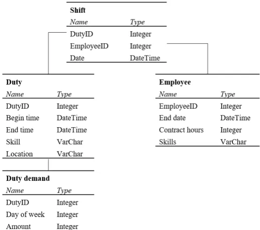
The historical data available contains the following data entities: i) Duties, ii) Shifts, iii) Duty Demand, iv) Employees, v) Historical shifts.

i Duties

Each customer’s database includes a set of duties,D. A duty is defined by one or multiple tasks with a begin- and end time in hours on a day. In some organizations, a duty also includes a required skill level and location. It is important to notice that a duty does not include a date. In this thesis, duties are indicated bya, or b, where a, b∈D.

ii Shift

A shift consists of a duty, a date and an employee that works the shift. iii Duty demand

The duty demand describes the number of shifts required with a specific duty for each day of the week. In this way, the duty demand is the same for all weeks. The planner can also change the duty demand for a specific week.

iv Employee

(20)

v Historical shift

A historical shift is a shift that took place in the past. In this thesis, historical shifts are indicated byh.

vi Historical shift schedule

[image:20.595.164.432.216.452.2]

The historical shift schedule,H, is the set of all historical shifts h. Figure 2.1 shows the relation between the data entities.

Figure 2.1: Relation between data entities used in this thesis

(21)

Table 2.1: Description of the scheduling problems of the customer cases Customer Number of

duties

Number of shifts per week

Number of employees

Total contracted hours (per week)

Length historical schedule (months)

A1 40 177 131 1795 60

B1 49 196 35 812 40

B2 36 112 40 1059 40

B3 65 93 30 732 40

C1 36 131 61 1395 48

C2 11 45 40 460 48

C3 43 161 76 1659 48

C4 36 131 62 1231 48

2.2 OWS Optimizer

This section introduces the categories of constraints used in the Optimizer, the way these con-straints are modeled, and the algorithm that solves the shift scheduling problem.

2.2.1 Constraints in OWS

OWS contains three types of constraints: i) Hard constraints, ii) Soft constraints and iii) Employee-wishes. All these constraints can be formulated on different levels within the organi-zation. The remaining of this section consists of a detailed description of each of the categories and the levels where the constraint can be formulated on.

i Hard constraints

Hard constraints can be formulated on the following four levels: (a) National level

Hard constraints on national level represent labor laws that apply to all employees in a country. An example of this constraint is the following WHA rule:

• ’An employee must have at least 13 free Sundays per year.’ (Ministerie van Sociale Zaken en Werkgelegenheid, 2010).

(b) Industry level

Hard constraints on industry level contain industry-specific rules, in The Netherlands also known as the Collective Labor Agreement (CLA). An example of such an agree-ment:

• An employee has the right to have at least 26 free weekends a year. (c) Department level

These constraints apply for all employees in a department, for example:

• An employee may work at most 3 night shifts in a row. (d) Individual level

Hard constraints on individual level apply for a specific employee, such as:

(22)

• Personal agreements, for example, an employee is not required to work at location B.

ii Soft constraints

Soft constraints can be formulated on the following two levels: (a) Department level

These soft constraints apply for all employees in a department, for example:

• A shift with duty type 1 should be followed by a shift with duty type 2. (b) Group level

Constraints formulated on group level hold for a specific group of employees within a department, for example, part-time employees. For example:

• Part-time employees should work at most 2 weekend shifts a month. iii Employee-wishes

Employee-wishes can either be modelled as a hard constraint or a soft constraint. Employ-ees can submit arequest not to work during a given period or a specific shift. Subsequently, the planner can decide if this wish should be modeled as a hard constraint or soft constraint. Additionally, employees canrequest to work during a given period or a specific shift. Since there is no guarantee that the preferred shift is available, arequest to work is always mod-eled as a soft constraint. If the employee-wish is modmod-eled as a soft constraint, planners must assign a weight to this employee-wish. Examples of employee-wishes are:

• An employee wishes a day-off on 01-01-2020.

• An employee wishes not to work on every other Monday.

• An employee wishes to work a night shift on Thursday.

In this research, the focus lies on identifying the parameters of soft constraints in historical shift schedules. Hard constraints and employee-wishes are out of scope for the following reasons: i) Hard constraints are derived from labor laws and collective agreements, and ii) Employee-wishes are requested by the employee. In other words, both hard constraints and employee-Employee-wishes are known, therefore there is no need to identify these constraint types based on historical data. However, as hard constraints define the boundaries of the soft constraints, we must keep the relation between the different categories of constraints in mind.

2.2.2 Model formulation

(23)

[image:23.595.88.508.157.473.2]

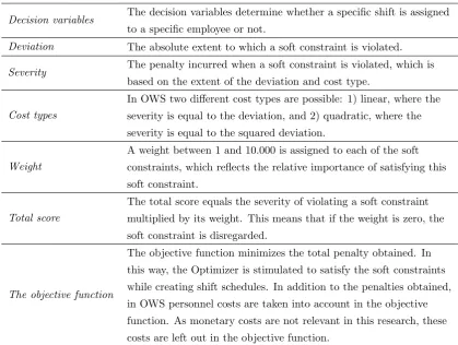
The Optimizer includes a set of soft constraints. The Optimizer collects all violations of a soft constraint for the given scheduling period. We define these violations as a set V, where a violationv∈V. The terminology of the Optimizer is listed in Table 2.2.

Table 2.2: Terminology OWS optimizer

Decision variables The decision variables determine whether a specific shift is assigned

to a specific employee or not.

Deviation The absolute extent to which a soft constraint is violated.

Severity The penalty incurred when a soft constraint is violated, which is

based on the extent of the deviation and cost type.

Cost types

In OWS two different cost types are possible: 1) linear, where the severity is equal to the deviation, and 2) quadratic, where the severity is equal to the squared deviation.

Weight

A weight between 1 and 10.000 is assigned to each of the soft constraints, which reflects the relative importance of satisfying this soft constraint.

Total score

The total score equals the severity of violating a soft constraint multiplied by its weight. This means that if the weight is zero, the soft constraint is disregarded.

The objective function

The objective function minimizes the total penalty obtained. In this way, the Optimizer is stimulated to satisfy the soft constraints while creating shift schedules. In addition to the penalties obtained, in OWS personnel costs are taken into account in the objective function. As monetary costs are not relevant in this research, these costs are left out in the objective function.

The objection function 1 of the Optimizer is to minimize the sum of all penalties obtained from violating soft constraints, i.e. the total score. Equation 2.1 shows the calculation for the

total score. The height of the penalty incurred from violating a soft constraint depends on i) The severity of the deviation and ii) The weight of the soft constraint. The severity of a deviation depends on the extent of the deviation and the cost type of a constraint, see Equation 2.2. The extent to which a constraint is violated depends on the preferences as defined by the customer and the realized shift schedule. For example, if a soft constraint defines that employees should work at most 1 night shift per week and the employee works 3 night shifts in a specific week, the deviation is equal to 2. The cost type is predefined for each constraint type and can either be linear or quadratic. In the case a constraint has linear costs, the severity is equal to the deviation. In the case a constraint has quadratic costs, the severity is equal to the squared deviation. By using quadratic costs larger deviations from the preferences are considered to be more severe.

1_{As monetary costs are not relevant in this research, the objective function in this research is the minimization}

(24)

T otalScore=X v∈V

Severityv∗W eightv (2.1)

Severity=

 



Deviation, In case of linear costs

Deviation2, In case of quadratic costs

(2.2)

2.2.3 Algorithm OWS

The Optimizer goes through the following four consecutive phases to generate a shift schedule: i) Greedy Insertion construction heuristic, ii) Genetic Algorithm, iii) Local optimization, iv) Ruin and recreate. A full description of the algorithm used in OWS can be found in (Post and Veltman, 2004).

1 Greedy Insertion construction heuristic

The objective of the first phase is to create a set of initial solutions. The user can define the number of initial solutions to create. First, all vacant shifts receive a score that represents the difficulty to schedule. This score is based on several criteria, for example, a weekend shift receives a higher score than a shift on a weekday. Thereafter, the list of vacant shifts is sorted in decreasing order of their score. A Greedy Insertion (GI) construction heuristic is used to assign every vacant shift to an employee in the sequence of the sorted list. To obtain several initial solutions, the GI is executed multiple times. In each iteration, the GI divides the employees over different subsets. Subsequently, as much as possible shifts are assigned to the employees in the first subset, then the remaining shifts are assigned to employees in the other subsets. By creating different subsets of employees, the GI can create different initial solutions.

2 Genetic Algorithm

Once the GI created a set of so-called parent solutions, the Genetic Algorithm (GA) will be initialized to generate children solutions. The GA uses five types of operators to generate new solutions: i) Two crossover operators, which combines two parent solutions into two child solutions, and ii) Three mutation operators, which transform one parent solution into one child solution. In each iteration, the GA randomly selects one of these five GA operators and applies this on one or two random parent solution(s). If the operator results in an infeasible child solution, a repair heuristic is applied to guarantee the feasibility of a solution. The children solutions are saved in a new set of solutions, where the GA is also applied. The GA continues with creating children solutions until the maximum computation time for global optimization is reached The best solution found so far is selected. The maximum computation time for global optimization can be defined by the user.

3 Local optimization

(25)

employees. When such a move results in a better solution, the new solution is accepted. Once a schedule cannot be improved anymore using 1-opt changes, the solution is 1-opt optimal and the algorithm starts a 2-opt search. If an improvement is found in the 2-opt search, the algorithm returns to the 1-opt search. When no improvements can be found for the 2-opt search, the 1-opt(k) search is initiated. In a 1-opt(k) search, k consecutive shifts are moved from one employee to another employee. Every time a better solution is found, the algorithm returns to the 1-opt search. The algorithm continues until it reaches 2-opt(3) optimality or when no improvements can be found within reasonable time. 4 Ruin & recreate

Finally, a ruin & recreate heuristic is applied to the best-found solution so far. By ruining and recreating the solution, the algorithm tries to escape from a local optimum. Two different operators exist to ruin the current solution. The first operator randomly selects a predefined number of employees using the roulette wheel principle: employees with a higher total penalty have a higher probability to be selected. All shifts within the scheduling period assigned to the selected employees will be removed. The second operator removes a predefined number of randomly selected shifts in the schedule. To recreate the solution, GI is applied to assign the vacant shifts to the available employees. One of the operators is randomly selected, where the probability is based on the success rate of previous iterations. The variable neighborhood search continues until the predefined total computation time is reached. The best-found solution is returned to the end-user and presented on the planning board.

2.3 Scheduling preferences

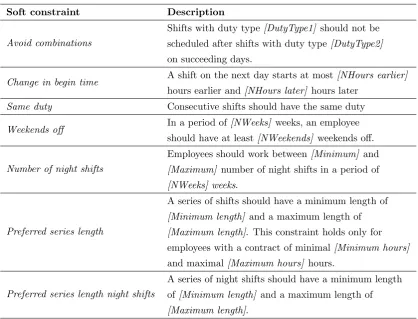
Data sets of eight departments from three different customers of ORTEC have been collected. As these customers currently use the Optimizer, their scheduling preferences and their corresponding soft constraints are known. In total seven different types of soft constraints are currently used by these customers. Table 2.3 provides an overview of these constraints and their description.

The first soft constraint type is Avoid combinations. For example, shifts with duty type E

should not be scheduled after shifts with duty typeL on succeeding days.

The second soft constraint type ischange in begin time. For example, a shift on the next day starts maximally 0.5 hours earlier and 1 hour later.

The third soft constraint type, same duty, indicates that two consecutive shifts should have the same duty. Consecutive shifts are shifts that are worked on two succeeding days by the same employee.

The fourth soft constraint type, weekends off, regulates the number of free weekends for employees. In this research a free weekend is defined as follows: an employee has a free weekend if no work takes place between Saturday 04:00 and Sunday 23:59. A customer can indicate a preference for both the number of free weekends and the number of weeks the constraint should consider, for example:

• Constraint 1: An employee should have at least 2 free weekends in a period of 4 weeks

(26)

Table 2.3: Categories of the soft constraints used at ORTEC’s customers

Soft constraint Description

Avoid combinations

Shifts with duty type[DutyType1] should not be scheduled after shifts with duty type[DutyType2]

on succeeding days.

Change in begin time A shift on the next day starts at most[NHours earlier]

hours earlier and[NHours later] hours later

Same duty Consecutive shifts should have the same duty

Weekends off In a period of[NWeeks] weeks, an employee

should have at least[NWeekends] weekends off.

Number of night shifts

[image:26.595.89.508.101.420.2]

Employees should work between[Minimum] and

[Maximum] number of night shifts in a period of

[NWeeks] weeks.

Preferred series length

A series of shifts should have a minimum length of

[Minimum length] and a maximum length of

[Maximum length]. This constraint holds only for employees with a contract of minimal[Minimum hours]

and maximal[Maximum hours] hours.

Preferred series length night shifts

A series of night shifts should have a minimum length of[Minimum length] and a maximum length of

[Maximum length].

The average number of free weekends is the same in both examples, however, example 2 is more strictly formulated. Figure 2.2 shows an example of a shift schedule for four consecutive weekends. In this example, constraint 1 is satisfied during the whole scheduling period. However, constraint 2 is violated, as the employee works both weekends in week 2 and 3. This results in a deviation of 1. In OWS, this constraints has quadratic costs, meaning that the deviation is squared.

Figure 2.2: Example constraint free weekends

The fifth soft constraint type isnumber of night shifts, for example: An employee should work between 2 and 3 night shifts in a period of 3 weeks. Figure 2.3 shows an example shift schedule for three weeks. In this period of three weeks, the employee works 4 night shifts, consequently, the deviation of the soft constraint is equal to 1 (= 4−3). In OWS this constraint type also has quadratic costs.

(27)

Figure 2.3: Example constraint number of shifts

length. A shift series includes shifts worked by the same employee on succeeding days. A series is interrupted if an employee does not work between 0:00 and 0:00 the next day. An example of such a constraint is: a series of shifts should have a minimum length of 2 and a maximum length of 3. Figure 2.4 shows an example of a shift schedule for two weeks including three shift series. In this example, the first shift series lies within the boundaries, the second shift series deviates 1 and the third shift series deviates 2. In OWS this constraint type has quadratic costs, therefore, the aforementioned example would result in a severity equal to 5 (= 12_{+ 2}2_).

Finally, customers indicate a preference for the series length of night shifts, this constraints works the same as the constraint Preferred series length. However, this constraint type takes only consecutive night shifts are taken into account.

Figure 2.4: Example constraint preferred series length

Table 2.4 summarizes the number of soft constraints used at each of the customer cases. This table shows that for each customer a different set soft constraints is relevant.

Table 2.4: Summary of the number of soft constraints used per customer case Customer

Soft constraint A1 B1 B2 B3 C1 C2 C3 C4

Avoid combination 8 - - - 2 - 6 4

Change in begin time - - - - 1 1 1 1

Same duty 1 - - - 1

-Weekends off - 1 1 1 - - -

-Number of night shifts 1 - - - 1 1 1 1

Preferred series length - 1 1 1 2 2 2 2

Preferred series length

(28)

2.4 Conclusion

This chapter describes the constraint types, the algorithm used in OWS and the soft constraints used at ORTEC’s customers. With this information, we can answer the following sub-research question:

How is the Optimizer currently used in OWS?

In OWS three constraint types exist: i) Hard constraints, ii) Soft constraints and iii) Employee wishes. In this thesis, the focus lies on identifying soft constraints. Soft constraints can be formulated both on department and group level.

In OWS, shift schedules are created by the Optimizer. The Optimizer goes through four consecutive heuristics to solve this optimization problem. The objective of the Optimizer is to minimize the total score, which consists of the sum of penalties obtained from violating and satisfying soft constraints. ORTEC’s customers typically use a combination of the following seven types of soft constraints:

• Avoid specific combinations of consecutive shifts

• Change in begin time of consecutive shifts

• Consecutive shifts should have the same duty

• The preferred number of weekends off

• The preferred number of night shifts

• The preferred series length

(29)

Chapter 3

Literature review

The objective of this research is to identify the scheduling preferences of customers based on historical shift schedules. The previous chapter describes soft constraints representing the cus-tomers’ scheduling preferences. The next step is to identify the parameters of these soft con-straints. To achieve this, literature is used to explore what already has been done in the fields of constraint learning. Section 3.1 provides an overview of relevant literature. Additionally, Section 3.2 discusses data mining techniques, which can be applied to discover interesting patterns in data sets (Han et al., 2012a). Finally, Section 3.3 provides an overview of frequently used eval-uation metrics in data mining that can be used to determine the performance of a data mining technique.

3.1 Constraint learning

In this section, we describe what has been done in the literature in the fields of constraint learning and use this as an inspiration for this research. Constraint learning refers to the problem of finding a set of constraints that is satisfied in a given data set (De Raedt et al., 2018). In other words, the constraints found should not be violated in the historical data set. First, we describe approaches to learn hard constraints from multi-dimensional data, such as the scheduling problem, followed by an overview of existing approaches to learn soft constraints.

(30)

shift types. Compared to ORTEC’s customers, where the number of shift types varies between 10 and 250 shift types, COUNT-OR was applied on a relative small scheduling problem. Both ModelSeeker and COUNT-OR aim to find the boundaries of hard constraints rather than soft constraints that represent the scheduling preferences. These methods set the parameters of the constraints equal to the extreme cases found in historical data, while in this research we aim to find frequently occurring patterns, therefore, these methods are not applicable in this research.

In contrast to learning hard constraints, relatively few approaches for learning soft constraints have been proposed in the literature. Approaches for learning soft constraints can be classified into two categories with different objectives: i) Learning the weights of the soft constraints and 2) Learning the structure of the soft constraints, where both the parameters as the weights of the constraints are being learned (De Raedt et al., 2018).

Rossi and Sperduti (2004) introduce an interactive framework to learn the weights of soft constraints. Within this framework, users rank constraints and solutions according to their pref-erence, subsequently, these scores are used to learn the relative weights of the given constraints (Rossi and Sperduti, 2004). A similar kind of approach was proposed by Teso et al. (2016), where interactive learning is used to the weights of soft constraints in customization and design prob-lems. In these two approaches, the set of relevant soft constraints including their parameters is given and only the relative importance of those soft constraints is being learned. In this research the parameters of the soft constraints are not known, therefore, we cannot use these approaches. Campigotto et al. (2015) propose a method, CLEO, to learn the structure of soft constraints. In this method, all possible soft constraints are enumerated. Subsequently, a weight is assigned to the soft constraints using the objective function. The objective function maximizes the utility of a schedule, where the utility is the sum of the weights of the satisfied constraints. Moreover, the objective function aims to set the weight of most of the constraints to zero, resulting, all irrelevant constraints are eliminated. Finally, in an interactive refinement phase, the parameters and weights of the constraints are tuned by human feedback. CLEO is tested in a setting with at most 9 types of soft constraints to enumerate. As ORTEC’s customers deal with complex scheduling problem, enumeration of all possible soft constraints would result in several hundreds of soft constraints. Moreover, CLEO requires human feedback during the refinement phase, while the objective of this research is to develop a method where no interaction with humans is required. To deal with a large number of constraints, Campigotto et al. (2011) suggest using known hard constraints to define the boundaries of the soft constraints to identify.

3.2 Data mining techniques

Data mining is a technique that can be applied to find interesting patterns in data sets. Han et al. (2012a) distinguish five types of data mining techniques to detect patterns in data sets: i) Data discrimination, ii) Frequent patterns, iii) Classification, iv) Cluster analysis and v) Outlier analysis.

(31)

distinguish desirable scheduling decisions from undesirable scheduling decisions, these would be the different classes in the data set. However, we do not know how these classes look like in advance. For this reason, data discrimination is no usable data technique in this thesis.

The second type isfrequent patterns and association mining, which extracts frequent patterns and associations between data objects from a data set. In this way, interesting relations between objects in a data set can be found. This technique is often used in marketing, for example, which products are often bought together? If we translate this example to our problem, this technique may help us to identify which combinations of shifts are often combined.

The third type isclassification, the process of finding a model that describes and distinguishes different classes. Based on characteristics of an object in the data set, the model provides a label to this object representing its class. The model is based on a training set, this set contains objects for which the class labels are known. In this research, we aim to find the scheduling preferences of customers. Since preferences are personal, each organization and department has unique preferences. Therefore, we do not have access to a training set including known preferences. For this reason, classification is no usable data technique in this thesis.

The fourth type is cluster analysis, which clusters objects in a data set based on their char-acteristics. In contrast to classification mining, clustering does not require a training set. In this research, cluster analysis might be useful to distinguish desirable patterns from undesirable patterns.

The fifth type is outlier analysis, where objects in a data set that do not comply with the general behavior are extracted. Outlier analysis is used in cases where rare events are interesting, for example in detecting fraudulent usage of credit cards. In this research, we are interested in frequent patterns in the data, as we assume that these frequent patterns represent the scheduling preferences. For this reason, we are not interested in the outliers. Therefore, outlier analysis is no usable data technique in this thesis.

Summarizing, in this research,frequent patterns and association mining andcluster analysis

are usable data techniques to detect frequent patterns in data sets. Section 3.2.1 provides a description of frequent patterns and association mining and Section 3.2.2 provides a description of cluster analysis.

3.2.1 Frequent patterns and association mining

Frequent pattern and associations can be extracted from data sets by using association rule mining. Association rule mining is a data mining technique to extract interesting correlations, frequent patterns pr associations among sets of items in a database (Kotsiantis and Kanellopou-los, 2006). The input of association rule mining is a data set with multiple observations. In association rule mining one observation is called a transactiont, where t∈T. Each transaction consists of an item set i including one or multiple items, where i ∈ I. Table 3.1 provides an example of a data set including three transactions and four different items. In this example, Transactiont1 includes the following item set: {i1, i3}.

In association rule mining, all possible item sets are created. The size of an item set is equal to

(32)

Table 3.1: Example of a data set including three transactions and four items

i1 i2 i3 i4

t1 1 0 1 0

t2 0 1 1 0

t3 1 1 1 1

this step item sets that occur infrequently are removed. Subsequently, association measures are calculated for each of the frequent item setsi. Finally, if the measures for an item seti satisfy a certain threshold, an association rule is created. In the remaining of this section, we explain these three steps more detailed.

1 Frequent item set generation

In general, the number of possible item sets i in a data set grows exponentially with the number of different items the data set contains: a data set that contains nitems can generate up to 2n_{–1 item sets (Tan et al., 2005). Consequently, the search space for frequent} item sets that need to be explored grows exponentially. In the literature, various ways to efficiently select frequent item sets have been explored. A commonly used approach is the Apriori principle, which is based on the following principle: ‘If an item set is frequent, then all of its subsets must also be frequent’ (Tan et al., 2005). For example, if item set{i2, i3} is frequent, then item set{i2}must also be frequent.

2 Association measures

Two important measures for association rules are support and confidence (Kotsiantis and Kanellopoulos, 2006). The support of an item set gives an idea of the frequency of that item set compared to all observationsN in the data set, see Equation 3.1. Association rules indicate an implication between items in a data set. For example, if a transaction contains

i1 there is a high probability that this transaction also containsi3. The rule of implication is formulated as follows: X →Y, whereX andY represent an item set. For each rule of implication, association measures can be calculated that can be used to eliminate irrelevant association rules.

Equation 3.2 shows the formula for thesupport of an item set. Lowsupport of an associa-tion rule indicates that the event occurred by chance. Therefore, the support reflects the usefulness of an association rule (Han et al., 2012b). Equation 3.3 shows the formula for the

confidence of an item set. Theconfidence reflects the certainty of an association rule. The

(33)

Kanellopoulos, 2006). In cases where the associations are directed, conviction is preferred over lift (Lin and Tseng, 2006).

Besides creating positive association rules, negative association rules can be created. Neg-ative association rules indicate which items conflict with each other (Wu et al., 2004). Equations 3.6 up to 3.10 represent the association measures for negative association min-ing. For example,support(X→ ¬Y), represents the support for transactions that include all items from item set X and does not include all items from item set Y.

Positive association mining measures

support(X) = f requency(X)

N (3.1)

support(X →Y) = f requency(X→Y)

N (3.2)

conf idence(X →Y) = f requency(X →Y)

f requency(X) (3.3)

lif t(X→Y) = support(X →Y)

support(Y) (3.4)

conviction(X →Y) = 1−support(Y)

1−conf idence(X →Y) (3.5)

Negative association mining measures

support(¬X) = 1−support(X) (3.6)

support(X → ¬Y) = f requency(X→ ¬Y)

N (3.7)

conf idence(X → ¬Y) = f requency(X → ¬Y)

f requency(X) (3.8)

lif t(X→ ¬Y) = support(X → ¬Y)

support(¬Y) (3.9)

conviction(X → ¬Y) = 1−support(¬Y)

1−conf idence(X → ¬Y) (3.10)

3 Rule selection

(34)

sets of different customers. Therefore, it is not possible to set a general minimum support threshold for all databases. Lin and Tseng (2006) propose a method to seek association rules with high confidence and a positive lift, without the need of a user-specified support threshold. The following three definitions are used to explain this method.

(a) Automated support threshold

An item setI={i1, i2, ..., in}is a frequent item set if the support of the item setI is larger than or equal to the lowest value of the support of the items inI, i.e,

support(I)≥min

i∈I support(i) (3.11)

(b) Strong association rules

Furthermore, Lin and Tseng (2006) define theminimum support of an itemi: ms(i). An association ruleX →Y is to be considered strong if the support of the association rule is larger than the lowest value of the minimum support of the items in the item set I, see Equation 3.12.

support(X →Y)≥ min

i∈X∪Yms(i) (3.12) The support of the items included in the item set,support(i), are ordered in ascending order. The minimum support of the items is calculated as follows:

ms(i) =  



support(i)∗support(i+ 1) if 1≤i≤n−1

support(i) if i=n

(3.13)

Additionally, to be considered strong, the confidence of an association rule must exceed a user-specified minimum confidence threshold, see Equation 3.14. Lin and Tseng (2006) use a minimum confidence threshold of 0.5.

conf idence(X →Y)≥M inimumConf idence (3.14)

(c) Interesting association rules

A strong association rule is also considered as interesting if the lift is greater than 1, see Equation 3.15. As lif t(X → Y)≥1 only holds if conviction(X →Y) ≥1, lift and conviction are replaceable in this definition. Therefore, although the direction of association is relevant in this thesis, using lift as a measure in this context is correct.

lif t(X→Y)≥1 (3.15)

3.2.2 Cluster Analysis

(35)

is not known on forehand. A frequently used partitioning method isK-Means clustering. The remaining of this section describesK-Means clustering based onCluster Analysis from Hair and Black (2000).

Within K-Means clustering, the objects, o, in a data set are represented in a Euclidean space. The K-Means algorithm clusters these objects into k clusters. The objective function of the algorithm used in K-Means clustering aims for high similarity within a cluster and low similarity between clusters. In other words, the objective is to minimize the total-within-cluster variation and maximize the between-cluster variation. Optimization of the total-within-cluster variation, SST otalW ithinCluster, is proven to be an NP-hard problem Hair and Black (2000). Therefore, in practice, a heuristic is often used to find a solution within reasonable time. The following steps are taken inK-Means clustering:

1 Scale all objects to an Euclidean space 2 Specify the number of clusters to create, K 3 Arbitrarily select K objects

The randomly selected objects represent the initial centers of the clusters, Ck. 4 Assign each observation to the closest center Ck

Subsequently, each object,o, in the data set is assigned to the closest center usingdistance(o, ck), the Euclidean distance between these points. The within-cluster-Sum of Squares (SS),

SS_kW ithinCluster, represents the quality of a clusterk and can be calculated as follows:

SS_kW ithinCluster= X o∈Ck

distance(o, ck)2 (3.16)

The total-within-cluster-SS equals:

SST otalW ithinCluster= K

X

k=1

SS_kW ithinCluster (3.17)

5 Update the cluster means

For each cluster k a new cluster center is calculated given the objects assigned to this cluster. Subsequently, all the objects are reassigned using the new cluster centers.

6 Continue until no improvement is found, or the maximum number of iterations has been reached

Additionally, TheSBetweenClusters_{indicates to what extent the clusters differ from each other.} TheSBetweenClusters _{is equal to the sum of squared distances between the centers, see Equation} 3.18. K-Means clustering aims for a lowSST otalW ithinCluster and a highSSBetweenClusters.

SSBetweenClusters= K

X

k=1 K

X

j=1

distance(ck, cj) (3.18)

(36)

• Simple and fast algorithm

• Can be applied effectively on small- to medium-size data sets and the followingdisadvantages:

• If the number of clusters K is unknown, it is difficult to determine number of clustersK

A method to overcome this problem is the elbow method. The elbow method is based on the following observation: increasing the number of clusters, reduces the number of objects assigned to each cluster and therefore can reduce the within-cluster variation of each cluster. However, the marginal reduction of the within-cluster variation may decrease if the number of clusters increases. In other words, at some point increasing the number of clusters does not have much effect on the solution. Consequently, the curve of the total within-cluster variation and the number of clusters formed shows a so-called ’elbow’. The number of clustersK is chosen as the turning point in this curve.

• The results depend on the initially randomly chosen centers

A drawback of the K-Means algorithm is that it does not have to converge to a global optimum and can terminate at a local optimum. Consequently, the results may be depen-dent on the initial random centers. Therefore, it is recommended to apply the K-Means multiple times with different initial centers and select the best-found solution.

• Sensitive to outliers

TheK-Means method is sensitive to outliers. Additionally, changing the order of the data may result in different clusters.

3.3 Evaluation of results

This section describes evaluation metrics to evaluate the performance of data mining techniques. This section is divided into two sub-sections. Section 3.3.1 describes evaluation metrics to eval-uate nominal variables. Nominal variables include mutually exclusive categories. For nominal values, the order between the categories does not matter. Section 3.3.2 describes evaluation met-rics to evaluate ratio variables. Ratio variables are non-categorical variables. For ratio variables, the order matters and the difference between two values is meaningful.

3.3.1 Nominal variables

As described before, nominal variables include mutually exclusive categories. Each of these categories is called a class. In classification problems, data mining techniques are used to assign a variable to one of these classes. Such a data mining technique is a so-called classifier. A confusion matrix, see Figure 3.1, helps to evaluate the performance of such a classifier. The example in Figure 3.1 shows a confusion matrix for a nominal variable including two classes, in other words, a binary variable. A confusion matrix can also be created for nominal variables including multiple classes.

We explain the confusion matrix using an example. An instance can take the value true or

(37)

Figure 3.1: Confusion matrix of a classification problem with two classes

is known. In the confusion matrix, the P and N represent the number of instances that are equal totrue and false, respectively. In a classification problem, the objective is to identify the value of an instance, without knowing its actual value. A classifier identifies the value for every instance. In the confusion matrix, theP’ andN’ represent the number of instances classified as

true orfalse, respectively. To determine the performance of a classifier, the actual and classified value of an instance is compared. For example, if the actual value of an instance is true and the instance is classified asfalse, the instance is labeled as false negative. Table 3.2 explains all definitions used in the confusion matrix. The confusion matrix can be used to calculate measures to evaluate the performance of a classifier method, in the remaining of this section we give a short description of these measures based on Han et al. (2012c).

Table 3.2: Definitions evaluation of classification method

True Positive (TP) The number of instances classified as true that are actual true

True Negative (TN) The number of instances classified as false that are actual false

False Negative (FN) The number of instances classified as false that are actual true

False Positive (FP) The number of instances classified as true that are actual false

P’ The number of instances classified as true

N’ The number of instances classified as false

P The number of instances that actual true

N The number of instances that actual false

The accuracy of the method is the percentage of variables that have been classified correctly, whereas, the error rate is the percentage of variables that have been classified incorrectly, see Equations 3.19 and 3.20. Accuracy and error rates give equal weight to false positives and false negatives, therefore, positive and negative instances should be of equal importance.

Other common methods to evaluate the model are recall and specificity, see Equations 3.21 and 3.22. The recall, also known as the true positive rate, is equal to the percentage of positives instances that have been classified positive. Recall is also known as a measure of completeness. In cases where it is important not to miss any true instances a high recall is required. The specificity, also known as the false positive rate, is equal to the percentage of false instances that have been classified false. Cases where it is important not to classify false instances as true require a high specificity. In general, methods with high recall, have a lower specificity.

(38)

weight to precision and recall, whereas theFβgivesβtimes more weight to recall as to precision. The aforementioned measures can be calculated as follows:

Accuracy= T P +T N

P+N (3.19)

Error= 1−Accuracy (3.20)

Recall=T P

P (3.21)

Specif icity= T N

N (3.22)

P recision= T P

T P +F P (3.23)

Fβ=

(1 +β)2∗precision∗recall

β2 _∗_precision ₊ _recall (3.24)

3.3.2 Ratio variables

This section describes metrics to evaluate the identified values of ratio variables based on Drakos (2018). A frequently used measure to evaluate continuous variables is the Mean Squared Error (MSE), see Equation 3.25. The MSE measures the average squared error of the identified values compared to the actual values. The Root Mean Squared Error (RMSE) is introduced to scale the errors to the same size of the target values and is equal to the root of the MSE, see Equation 3.26. As the error in the MSE and the RMSE is squared, both methods penalize bigger errors more than smaller errors. The Mean Absolute Error (MAE) takes the absolute values of the errors without squaring them, see Equation 3.27. Therefore, the MAE is less sensitive to outliers compared to RMSE and MSE.

Based on MSE, RMSE or MAE it is difficult to determine to what extent the method can identify the right values. The coefficient of determination,R2_{, compares the performance of the} model and a baseline model, see Equation 3.28. The baseline model is the simplest possible model, for example, setting the identified value equal to the average of all items. The value of

R2 lies between−∞and 1, a negative value indicates that the model is worse than the baseline model, a value close to 0 indicates that the performance of the model is close to the performance of the baseline model and a value close to 1 means that the model has almost zero error.

M SE = 1

N

X

i=1

(yi− yˆi)2 (3.25)

RM SE=√M SE (3.26)

M AE= 1

N

X

i=1

|yi− yˆi| (3.27)

R2= 1− M SE(model)

(39)

3.4 Conclusion

The objective of this chapter is to answer the following research question: What can we learn from the literature about identifying preferences from data? The following sub-questions have been answered in this chapter:

a What techniques exist to learn soft constraints from historical data?

Relatively few approaches exist to learn soft constraints from historical data. In most ap-proaches, user-feedback is required or only the weights of the constraints are being learned. As this research aims to identify the parameters of soft constraints without using user-feedback, these existing approaches cannot be applied in this research. Additionally, the described approaches tackle small theoretical problems rather than complex real-world problems.

As suggested by Campigotto et al. (2011), known hard constraints can be used to reduce the solution space of complex problems, and thus the number of possible solutions. Using hard constraints, therefore, helps to structure complex problems and can be used to determine the boundaries of the soft constraints. This allows for a more targeted search for soft constraints within the data.

b What data mining techniques can be used to identify preferences from data?

Data mining is the process of identifying interesting patterns in data sets. The literature describes several categories of interesting patterns. Two of these patterns are frequent patterns and associations mining and cluster analysis. First, association rule mining can be applied to identify frequent and infrequent item sets from data sets. In Chapter 1, the assumption was made that historical shift schedules contain implicit preferences. We assume that desirable scheduling decisions were made frequently. Mining frequent patterns helps us to identify these frequently made scheduling decisions. Furthermore, infrequent patterns could indicate undesirable scheduling decisions. Second,K-Means clustering is a data mining technique to cluster objects in a data set based on their characteristics. This technique could help us to cluster employees within a scheduling department, as different preferences may exist for part-time and full-time employees.

c What evaluation metrics are available to determine the performance of a data mining tech-nique?

(40)

Chapter 4

Problem approach

Chapter 2 describes types of soft constraints used by ORTEC’s customers who currently use the Optimizer. In this chapter, we propose a method to identify the parameters of these soft constraints. As described in Chapter 1, the objective is to use both historical shift schedules and domain knowledge to identify scheduling preferences of ORTEC’s customers. With domain knowledge, we mean specific knowledge about shift scheduling in practice, for example, labor laws and known preferences. Adding domain knowledge to the data mining technique prevents us from suggesting irrelevant constraints to the customer and could improve the performance of the method we propose. Figure 4.1 shows a schematic overview of the problem approach.

Figure 4.1: Schematic overview of the problem approach

Preference learning: What defines an optimal shift schedule?