Determining Bed Capacity using Mathematical Optimization

(1)

University Medical Center Utrecht

University Of Twente

Bachelor Thesis Industrial Engineering and Management

Determining Bed Capacity using

Mathematical Optimization

Author Hayo Bos

[email protected]

Supervisors Dr.ir.A.G. Maan-Leeftink(UT) Dr.D.Demirtas (UT) Drs. R.H.A. Maas (UMCU)

(2)

(3)

Preface

The report in front of you concludes my bachelor assignment which I conducted at Neu-rology and Neurosurgery department of the University Medical Center of Utrecht. It also concludes my bachelor study Industrial Engineering and Management and therewith my period at the University of Twente. It is the result of five months of hard work, in which I have learned how it is to be working for a large, complex organization with people who look from a totally different angle to certain subjects as I do. I have experienced my time at UMCU as fun and a valuable addition to my track record.

I want to thank both my supervisors Gr´eanne and Derya for the feedback they have provided, their flexibility and their ideas to further improve my thesis. Besides that, I want to thank Rob and Janet for their approachability and willingness to help me when I got stuck. I want to thank Michel for his comments and readiness to be a sparring partner when needed and my boyfriend Quinten for his feedback and support during the writing process. Lastly, I want to thank my sister Nienke for her inspiration and time to make my thesis to what it has become.

I hope you will enjoy reading my thesis.

(8)

(9)

Management Summary

Introduction and Problem Analysis

University Medical Center of Utrecht’s (UMCU) brain division houses three clinical wards and two Medium Care Units (MCUs). Two of these clinical wards and both MCUs are central in this research. In these wards there is too much variability in bed utilization, and too many patients are being declined due to a fully occupied ward. Besides that, a lot of incident reports are due to communication errors between the professionals of the different wards. To solve these problems, the management has decided to merge both MCUs and clinical wards. This intervention alone would not solve all problems. After a thorough analysis, we have discovered that the management lacks understanding of the (quantitative) relation between the bed occupancy and bed blocking probability. In order to solve the problems mentioned, we thus need to provide information on the optimal bed capacity and its relation with relevant Key Performance Indicators (KPIs). The central problem is therefore formulated as:

“What is the optimal number of beds for the new wards, taking the relevant KPIs into account?”

Method

(10)

Contents

Results

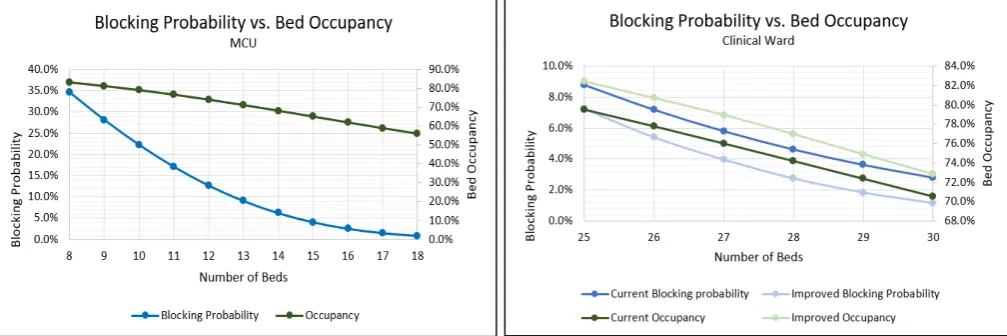
[image:10.595.68.572.162.330.2]

Using the models of the previous section, we calculated the relation between the blocking probability and bed occupancy given a number of beds. This relation is pictured in Figure 1.

Figure 1.: The relation between the blocking probability and bed occupancy for a given number of beds for the MCU (left) and clinical ward (right).

From this figure we can derive that, if we want to meet the target, we need at least 16 beds for the MCU resulting in a bed occupancy of about 62%. For the clinical ward we pictured both the current situation (dark colors) as well as the situation after altering the elective arrivals (light colors). To meet the target blocking probability we now need 28 beds with a bed occupancy of 74%. If however the management is able to stabilize elective arrivals through the week (including the weekend), we need 27 beds for a lower blocking probability resulting in a bed occupancy of about 79%. Furthermore, we remark that for all set-ups altering the elective arrivals results in a higher bed occupancy and lower blocking probability.

Recommendations

We have translated the described analysis into workable recommendations which are presented below.

•We recommend to base the number of required beds for the new ward and MCU on a quantitative method as ours rather than solely using a target occupancy and averages. Given the desired rejection rate of 3% for the MCU and 5% for the clinical ward, we advise a bed capacity of 16 and 28 beds respectively.

•The variability in elective arrivals should be reduced as much as possible. Ideally, the number of elective arrivals should be equal per day per week.

(11)

Contents

•Capacity decisions should be based on the entire distribution of the relevant variables rather than averages (to avoid the well-known “the flaw of averages”). This means that UMCU should use decision models (e.g., from Operations Research) for capacity problems, that use the underlying variability of the data instead of simple rules of thumb that only use averages.

(12)

(13)

Definitions, Abbreviations and Notation

Definitions

• Clinical ward: A room or group of rooms with beds to provide regular care to patients.

•MCU/Step Down Unit: Medium Care Unit; a special ward providing care of a level between the Intensive Care and the clinical ward. Within the Neurology & Neurosurgery department, the MCU also has a stroke unit for emergency patients.

•Bed blocking probability / Probability of refusal: The probability that a patient can not be treated where he/she should be treated because all beds are occupied.

• The management: The main group of stakeholders within UMCU who are entitled to make the decisions, for example about bed capacity, the decision for which this thesis gives advice.

Abbreviations

• ALOS: Average Length Of Stay

• CI: Confidence Interval

• CV: Coefficient of Variation

• ICU: Intensive Care Unit

• KPI: Key Performance Indicator

• LOS: Length of Stay

• MCU: Medium Care Unit

• MOL: Modified Offered Load

• MSER: Marginal Standard Error Rule

• N&N:Neurology and Neurosurgery

• OR: Operations Research

• PCIR: Patient Care Incident Report

• SMEs: Subject Matter Experts

(14)

Contents

Notation

Symbol Definition

n The number of replications in a simulation study. ¯

X Sample mean.

S Sample standard deviation.

τ Lexis ratio.

k, K Subgroup and total number of subgroups respectively.

t, T Moment in time (e.g., day of the week) and total time span under consideration respectively.

s, c Number of beds under considerations, and maximum number of beds respectively. Bt,B¯ Blocking probability on t, average blocking probability.

µk

Parameter of hyperexponential distribution, µ−_i 1 is the mean of subgroup k.

pk

Parameter of hyperexponential distribution, pk is the fractional size of subgroup k.

λt Arrival rate on timet.

Λ Total arrival rate overT.

mk(t) Offered load (i.e., patients present) of subgroup kon timet. m(t) Total offered load on time t.

m∗(t) Target load on t.

ci_t Constant.

¯

X Sample mean.

S Sample standard deviation.

tn−1,1−1/2α

[image:14.595.118.482.111.466.2]

The Student-t distribution with n−1 degrees of freedom, and a significance level of α.

Table 1.: Definitions of mathematical symbols.

(15)

1. Context Analysis and Problem

Formulation

In this chapter we describe the problem statement. We use a problem cluster by which we analyse what the core problem is, which will be the common thread throughout thesis.

1.1. The University Medical centre of Utrecht

University Medical centre of Utrecht (UMCU) is one of the eight university medical centres of the Netherlands. UMCU employs more than eleven thousand people, and provides care to more than thirty thousand patients a year. Within UMCU, there are twelve divisions corresponding to their function. One of these divisions is the brain di-vision. The brain division is divided into four departments: Psychiatry, Neurology and Neurosurgery, Rehabilitation Physiotherapy Science & Sport and Translational Neuro-science. This assignment takes place in the Neurology and Neurosurgery department (N&N). The N&N department is divided into seven care units which groups patients according to their clinical status of diagnoses, see Figure 1.1.

1.1.1. Wards

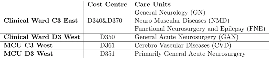
Within the N&N department, there are three clinical wards and two Medium-Care Units (MCUs). For this assignment, two clinical wards and both MCUs are considered. These wards correspond to one or multiple cost centre(s)1. The distribution of care units over the different wards and the wards’ cost centres are given in Table 1.1.

1.1.2. Merger

The management of the N&N department has encountered several problems. There is a deficit of 2.3 million euros, nurses experience a lot of variability in bed demand and patients are being refused due to lack of beds at certain moments. Furthermore, there are a lot of Patient Care Incident Reports (PCIR)2 _{regarding communication between}

(medical) professionals. As an attempt to solve these problems, the management has decided to merge two of its wards (C3 East and D3 West) and join its MCUs. The required capacity is yet unknown, and is one of the reasons for this research.

1

kostenplaats

(16)

1. Context Analysis and Problem Formulation

Cost Centre Care Units

Clinical Ward C3 East D340&D370

General Neurology (GN)

Neuro Muscular Diseases (NMD)

Functional Neurosurgery and Epilepsy (FNE)

Clinical Ward D3 West D350 General Acute Neurosurgery (GAN)

MCU C3 West D361 Cerebro Vascular Diseases (CVD)

[image:16.595.119.574.83.180.2]

MCU D3 West D351 Primarily General Acute Neurosurgery

Table 1.1.: The link between the wards, the care units and the cost centres of the Brain division.

The relation between and context of the mentioned problems is further investigated within the next section.

Figure 1.1.: The organigram of the Brain division of UMCU.

[image:16.595.183.471.274.544.2]

(17)

1.2. Problem Definition

This section explains the managerial problems that triggered this research. Subsequently, it will be clarified how these problems lead us to the core problem. The two management problems that are central in this assignment are

“There are patients who are declined or placed within another division”

-and-“There is too much variability in bed demand”

These problems signaled the management that the care giving process is not efficient enough. Since the causes of these managerial problems are yet unclear, we need to distract the core problem. To do so, we will use the method provided of Heerkens and Van Winden (2011:44-50). Roughly this method consists of analyzing the problems’ context by means of a problem cluster, and then select the core problem based on several criteria. The graphical illustration of the problem cluster can be found in Appendix A. The explanation of this figure is given in the text below. To start, we analyse the management problems and subsequently how they share partly the same cause, which happens to be the core problem of this assignment.

1.2.1. Rejection of Patients

The fact that patients are declined is caused by having no unoccupied beds which is in turn caused by the fact that on a certain moment, the number of beds is too low. This does not necessarily mean that the number of beds should be higher, since the bed demand fluctuates over time. However, to correctly determine the number of beds needed good understanding of the relation between the fraction of patients that are declined and the bed utilization is required. The management has indicated that they lack this knowledge. For instance, the management does know that it does not want too many patients to be refused but they can not tell the desired and current number of refusals. After all, having no declined patients is not reasonable due to the stochastic nature of patient arrivals. The above boils down to an absence of knowledge about the trade-off between bed utilization and patient refusals. Due to this lack of insight, it could be that the number of beds is too high because the number of rejections is actually (very) low. This would lead to overcapacity which is a waste of money. This in turn leads to an increase of the deficit. All in all, the management needs understanding of the bed utilization and capacity and its relation with patient refusals, because now it is likely that the number of beds is either too high or too low.

1.2.2. Variability in Bed Demand

(18)

We observed three causes of the variability of bed demand. The first is that admissions take place before discharges. This causes peak demand for beds, which increases the variability. The second is that the current wards and MCUs are too small. This is an additional reason that led to the decision to merge both wards and MCUs. The third reason is that it is not entirely clear how to measure bed occupancy and it means. One can thus say that the management lacks knowledge about bed capacity management. There is also no knowledge about which type of patients (elective or scheduled) exactly cause the variability in bed demand.

The lack of insight into the bed capacity has in turn several causes. One of them is that there is no registration of beds that are closed that day. This means that the utilization of beds as reported by the information system is much lower than in reality. Another cause is that there is variability in the arrival of patients which makes the process complex.

1.2.3. The Core Problem

The next step is to select the core problem. We will do so following the guidelines of Heerkens and Van Winden (2011:48). The main idea is to go “back” in the problem cluster to the first problem that can be solved and has no external causes. This leaves us two candidates: “There is no registration of beds that are closed” and “There is a lot of variability in the arrivals of patients”. The first is not suitable as this is something the department is already working on. The latter is not suitable because we cannot change the way most patients arrive. Therefore this problem is not really solvable which is why these are not suitable candidates (Heerkens and Van Winden, 2011:48). The variability of elective patients could be decreased when using a better way of scheduling based on the pattern of emergency patients, but the department would first prefer to have better insight in what would be the optimal number of beds (where these patterns probably also play a role). This argument, together with the fact that the first candidate is not suitable, results in moving forward one step in the cluster. Since, as said before, the management is eager to gain this knowledge and it is the first suitable problem in the cluster we decided let this be the core problem. Resembling the above, the core problem is formulated as:

“The management does not have enough understanding of the different variables that play a role when determining the bed capacity”

Solving this problem will help the management to decide on the bed capacity for the merged ward and joined MCU.

1.2.4. Scope

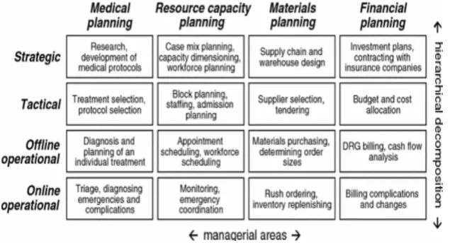
This section serves to define the scope of this research which is determined using the framework of Hans et al.(2011). A picture of this framework is given in Figure 1.2. The research focuses on determining the bed capacity for the new ward and the MCU. Following the framework this corresponds to “Resource capacity planning” on strategic

(19)

1.3. Knowledge problem and Research Questions

[image:19.595.111.429.319.491.2]

level. Using the framework, we underpin further scope conditions. First of all, the implementation and evaluation is not part of this assignment. The management has indicated that the advice will (most likely) be taken into account when the rebuilding of the nursing wards and MCUs takes place. This will not be until 2019, which is outside the time window of this assignment. Secondly, the scheduling of personnel is not taken into account. This corresponds well to the framework of Hans et al.(2011), since personnel planning belongs to the “Offline Operational” level. Third, the allocation of care units to wards is assumed to be fixed. The management has indicated that the decision making regarding the assignment of care units to wards has been completed and should not be revised. Fourth, the research most likely will not entail admission scheduling which is planning on the tactical level (Hans et al.,2011). The number of admissions allowed heavily depends on other parts of the chain, like operation room planning. Studying this aspect is not feasible within the given time frame as it is a fairly complex process. The intended deliverable is, as stated in the previous subsection, insight into the bed utilization and its relation with relevant variables given historical data. It will not be a real time tool to plan day-to-day bed capacity.

Figure 1.2.: The framework of Hans et al. (2011).

1.3. Knowledge problem and Research Questions

1.3.1. Research Aim

(20)

1.3.2. Knowledge problem

Solving the problem stated in the previous section requires knowledge. This knowl-edge will be acquired by following the information strategy when one faces a knowlknowl-edge problem. The knowledge problem in this assignment is formulated as:

“What is the optimal number of beds for the new wards taking the relevant KPIs into account?”

Answering this question will provide the required understanding of the bed capacity and occupancy.

1.3.3. Research Questions

To solve the knowledge problem, we break the problem down into smaller sub prob-lems which are presented below research questions. These research questions are the foundation of this thesis.

Current situation

First, we have to get insight about the current situation. The management indicated that there is no consensus over how many beds are optimal. A first step to provide insight is to determine what “optimal” in this context exactly means. The first research question serves to shed some light on this:

1: What is the current performance with respect to bed capacity on both wards and MCUs? (Ch.2)

a: What are the most important Key Performance Indicators (KPIs) regarding bed capacity, and how do both bed wards and MCUs perform now?

b: What are the desired levels of the KPIs ?

Then it should investigated what the arrival process looks like. What are the care pathways? Is there a difference between elective and emergency patients? One should also think of the statistical properties of the arrival time- and service time distribution. The next question deals with these issues.

2: What are the characteristics of the patient related processes? (Ch.2) a: What are the patient care pathways?

b: What are the statistical properties of the arrival and service process according to historical data?

3. What are the characteristics of the clinical ward and MCU after the merger? (Ch.3)

Literature

To prevent ourselves from reinventing the wheel, we look at work from other researchers about this topic. The one question we answer in this section is:

(21)

1.3. Knowledge problem and Research Questions

4: How to correctly determine the right number of beds on wards and MCUs according to the literature?(Ch.4)

Desired situation

To apply the theory and models, we will try to estimate their performance. To do so, we will test different configurations. Thereafter we will summarize the findings of this research with the final research question. Therefore, the last two research questions are:

5: What is the quantitative relation between the relevant KPIs when de-termining the required bed capacity? (Ch.5)

a: What are the scenarios to test? b: How do these scenarios perform?

(22)

(23)

2. Analysis of the Current Situation

In this section we investigate the current situation on the discussed wards and MCUs. First, the patient flows towards and in between the wards and MCUs will be discussed. Then, relevant concepts and Key Performance Indicators (KPIs) will be defined. Sub-sequently we will use UMCU’s database, called the data cube hereafter, to analyse the arrival process in more depth and develop understanding about the length of stay of the patients. The descriptives of the data used from the data cube can be found in the caption of the relevant figures and tables.

2.1. Patient Flows and Context

This section serves to shed light on the various patient flows. This will be done by considering three dimensions: the type of admissions, whether an admission is planned or not and whether a patient is assigned to the proper ward. Furthermore the arrival process is discussed. As a last subject, the typical patients and ward characteristics are discussed.

2.1.1. Type of Admissions

Patient admissions can be split up into new and transfer arrivals. Transfer arrivals encompass patients that are admitted on the concerning ward after an admission on another ward. Suppose a patient is admitted on the Intensive Care Unit (ICU) after receiving surgery and after some time (e.g., when the patient’s physical condition is more stable) the patient is transferred to the clinical ward. In this example, the new arrival is registered at the ICU, and the transfer arrival is registered at the clinical ward. Both the clinical wards and MCUs have both type of admissions. Moreover, part of the transfer admissions of the wards are caused by transfers from the MCUs to the clinical ward and vice versa. In the sequel, both transfer- and external arrivals are considered.

2.1.2. Elective and Emergency Patients

(24)

2. Analysis of the Current Situation

2.1.3. Diverted Patients

A third way to look at patient inflow, is to consider whether the ward of admission is the one where the patient should be admitted. Consider the patient with head trauma again. After arrival, the patient needs observation of the neurologist. Ideally, the patient is placed on the D340&D370 ward. Now suppose that this ward is occupied, and that the patient is diverted to the D350 ward, or even worse a ward in another division or hospital. The patient is then admitted on a “wrong” bed. The number of patients on wrong beds should be kept as small as possible both from a cost and a quality of care point of view. This means that a ward should not be fully occupied when a patient arrives.

2.1.4. The Arrival Process

Before admission, a patient goes through several steps. Most of the emergency patients arrive at the hospital via the Emergency Department (ED) or the outpatient clinic1. If a patient needs to be admitted, a doctor of the regarding department is contacted. This doctor in turn contacts the coordinating nurse who tries to find a free bed on the correct clinical ward or if this is not possible on another ward within the department. If it turns out that all of the above mentioned beds are occupied UMCU’s bed coordinator tries to find a bed somewhere else within the hospital. If this also fails, the patient is redirected to another hospital. Elective patients are directly admitted on the ward of destination. An elective patient makes an appointment and the staff reserves a bed. If, due to an unforeseen event (such as an unusual number of emergency arrivals) there is no bed available anymore, the elective patient is canceled.

2.1.5. The Clinical wards

As mentioned in Chapter 1 there are two clinical wards under consideration. The max-imum bed capacity on these wards is 18 beds for the D340&D370 ward and 12 beds for the D350 ward. Most of the days however, some of these beds are “closed”. As said before, the number of beds that is closed per day is not available in the data cube. This decision is made every morning when a group of nurses discuss the expected arrivals, discharges and transfers of that day. The beds are distributed over rooms, which are in turn located close to each other. A typical aspect of the first ward is the relatively high number of short stays. This is caused by the fact that there are many day treatments on this ward. The second ward has many (neuro) surgical patients which are e.g., admitted on the ward, receive surgery and subsequently are transferred back. In the desired future situation these two wards become one ward.

2.1.6. The Medium Care Units

Besides the clinical wards, also two Medium Care Units (MCUs) are under study: the D361 MCU and the D351 MCU. The MCUs have a capacity of 7 and 6 beds respectively.

1_Polikliniek

(25)

2.2. Performance Indicators

Noteworthy is that the first MCU is a stroke unit, which consists of beds reserved for patients with a stroke. Because the level of care is higher than clinical wards (hence the prefix medium), there are more nurses per patient. Similar to the clinical wards, the number of beds in use varies per day. Similar to the clinical wards, the MCUs will be combined.

2.2. Performance Indicators

There are many indicators for performance in healthcare regarding bed capacity. A selection of them is used in this thesis, on which we elaborate below. For each KPI we first explain what is measured and then how it is calculated.

2.2.1. Length Of Stay

The length of stay (LOS) is the time that passes between the moment that a patient is assigned to a hospital bed on a ward and the moment that patient is discharged. It is important to keep in mind that discharge in our context could also mean the transfer to e.g., the operation room, the MCU, the ICU etc.,contrary to the commonly used definition of discharge which is to be discharged from the hospital. To measure the LOS per patient, we do consider transfers. For example, suppose that a patient stays 3 days on Ward A and 4 days on Ward B. According to our intuition, this results in two LOS data points, being 3 days for ward A and 4 days for ward B (contrary to summing them). The LOS is an important KPI because it can be used used in the calculation of bed occupancy as we will see later, and thus is related with decisions regarding the number of beds. The financial controller of the department calculates the average length of stay (ALOS) as:

ALOS = T otal LOS

N umber Of N ew Admissions (2.1)

This overestimates the “real” LOS because the transfer patients are not taken into account. UMCU’s Business Intelligence division also provides information on the LOS. They do take the transfers into account, but again only provide averages. It is well known that (capacity) decisions in general should not be based purely on averages (also known as “The flaw of averages”) but rather on the underlying distribution. This will be further investigated in Section 2.4. The equation used to determine the ALOS in the sequel of this thesis is:

ALOS = T otal LOS

N umber Of N ew Admissions + T ransf er Admissions (2.2)

2.2.2. Rejection Rate

(26)

beds occupied. The rejection rate is defined as follows:

Rejection Rate= N umber of Rejected P atients

T otal N umber of Arrivals (2.3)

This is an important KPI in bed capacity decisions. Unfortunately, this KPI is not (yet) being monitored because it is hard to keep track of the number of patients that is re-jected. We should therefore analyse the data to calculate the current performance.There is no log of patients that are rejected. The same goes for the total number of arrivals, because only the admissions are being registered (i.e., the number of patient that do not find the ward fully occupied). The best thing that can be done is to estimate the current performance by estimating the fraction of time the wards are fully occupied.

2.2.3. Bed Occupancy

The last KPI that will be discussed is the bed occupancy. This is probably the hardest KPI to define, because there is no consensus both in the literature and at UMCU on how to calculate this ratio. It is an important KPI because in many hospitals it plays a central role in determining the number of beds needed (which in fact is strongly advised against by e.g., Green (2002)). Intuitively, one would say that bed occupancy is calculated as the capacity in use divided by the total capacity available (as one would usually define occupancy or utilization). Following this reasoning, the occupancy then can be defined as:

Bed Occupancyt=

N umber of P atients P resentt

N umber of Beds Availablet

∗100% (2.4)

Where the t indicates the time at which we evaluate the KPI (e.g., hour of the day). Following this definition, two difficulties arise. The first is that it is hard to measure the number of patients present at a given time. Time is a continuous parameter, and giving a precise measurement of bed occupancy would require continuous measurements which are not available in the data cube. The data cube does provide data on the number of patients present per 15 minutes. This data however is highly sensitive for input errors. An example of an input error is when a patient is already discharged but not registered as such, because the person in charge of this first had other things to do. Besides that, sometimes a patient is not physically present whereas he is registered as such. This can be the case when someone has completed his take-in for surgery, and can wait the days at home. The system then registers the patient as being present, whereas he does not occupy a bed. Reasoning this, the bed occupancy can be higher than 100%. The second difficulty is that beds are some days “closed” but for the previous years this has not been registered. It should be noted that the department is working on this, and does monitor the beds that are open/closed since a couple of months. The previous analysis underpins the need for another, more objective, estimator for the bed occupancy.

A well known result often used in Operations Research is Little’s Law (Little, 1961). It is formulated as follows:

L=λW (2.5)

(27)

2.3. Arrivals

With L being the number of customers present, λ being the arrival rate per time unit and W being the average length of stay. This equation is used in the same context as ours by e.g., De Bruin et al. (2009) and Cochran and Roche (2008). We could define λ as the arrival rate of patients per day and Las the number of patients present in steady state. Define c as the average open beds on day. Combining equation 2.4 and 2.5 then results in:

Bed Occupancy= λALOS

c (2.6)

2.3. Arrivals

In this section the patient arrival process will be analysed in depth. We do so by splitting the admissions into emergency and elective admissions (see Section 2.4). This is a useful distinction because especially unexpected arrivals (i.e., emergency arrivals) tend to be well described by a Poisson process (Young, 1965). The Poisson process will be explained in more depth below. Furthermore De Bruin et al. (2009) discovered that in a hospital situation also the planned arrivals (i.e., elective arrivals) are well described by a Poisson process. First the Poisson process will be explained as it plays a central role in this section. Subsequently we look at the arrival patterns of patients per ward (both elective and emergency), at the arrivals per day of the week and finally at the arrivals per hour of the day. It should be noted that the D351 ward was closed the first few weeks of 2017. This has been taken account for during all further analyses in the sequel of this thesis.

2.3.1. Poisson Process

Let N(t) be the number of arrivals up to timet≥0 (so N(3) is the number of arrivals up to and includingt= 3). If the following (mild) assumptions hold, number of arrivals in a specified interval N(t+s)−N(t) tend to have several interesting properties.

Assumptions:

1. The probability that 2 or more customers (patients) arrive at exactly the same time is 0.

2. The number of arrivals in non-overlapping time intervals is independent

3. In case of a stationary Poisson process: the distribution ofN(t+s)−N(t) is indepen-dent oft (i.e., the probability of 6 arrivals today is equal to the probability of 6 arrivals eight days from now).

If the above assumptions hold, then N(t+s)−N(t) (the number of arrivals in an interval of length s) follows a Poisson distribution with parameter λs = E[N(s)] and λ=E[N(1)]. Moreover, the inter-arrival times (the time between subsequent arrivals) tend to have follow an exponential distribution (Law, 2015:380-384). In other words, using the theory above, we can draw inferences about the arrival patterns. It is not hard to conclude that this property is very useful in capacity related problems.

(28)

between 7:00 AM and 09:00 AM), assumption 3 is violated. We then could be dealing with a non-stationary Poisson process (Law, 2015:380-384) (which turns out to be the case in our situation). In this case, we should specify the arrival rate as a function of the time (e.g., day of the week). Techniques for doing this will be discussed in Chapter 4.

2.3.2. Arrivals Per Ward

Elective Arrivals

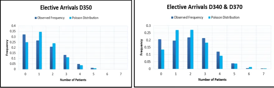
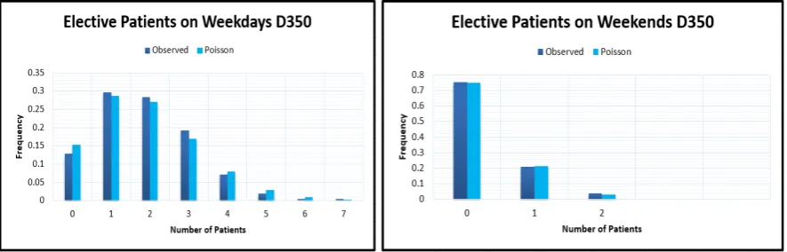
[image:28.595.119.559.415.556.2]

To analyse the arrival pattern per ward, we counted the number of emergency and elective arrivals on each day of the year 2017. Both new arrivals and transfers are taken into consideration, since also transfers are patient arrivals. Subsequently, the data was used to calculate summary statistics, and to draw a histogram. A histogram can be seen as a draft of the underlying probability distribution. Because a Poisson distribution (see Appendix B.1) is suspected, this distribution is “fitted” through the data to check whether Poisson arrivals are reasonable on first sight. The estimator of the parameter of the Poisson distribution used is the sample average X. This is also the Maximum Likelihood Estimator (MLE) and thus has several desirable properties (for more information see Appendix B.4). For both the clinical wards (D340&D370 and D350) the histograms can be found in Figure 2.1. It turns out that the frequency of 0 elective arrivals on a day seems to be a bit high. By visual inspection it is clear that the Poisson model underestimates this frequency and therefore we do not need a statistical test to verify this. The high frequency of 0 arrivals could be caused by the fact that

Figure 2.1.: Histogram of the elective arrivals on the clinical wards in 2017. Data re-trieved from data cube, n=363 (days) and n=362 respectively.

there are (basically) no planned admissions on weekend days and holidays2. Splitting the elective arrivals of the clinical wards into week- and weekend arrivals (where holidays onweekdaysare excluded) gave the histograms of Figure 2.2.

2

First- and second day of Christmas, Easter and Pentecost, New Years day, Ascension day and the day after, Good Friday and Kingsday

(29)

[image:29.595.60.503.84.226.2]

2.3. Arrivals

Figure 2.2.: Daily elective arrivals of the ward D350 after being split into week- and weekend days in 2017. Data retrieved from the data cube, n=250 and n=105 respectively.

This provides a much better fit (see Table 2.1 for the p-values the χ2 _{goodness-of-fit}

test) for the elective arrivals for the D350 ward. The histograms for elective arrivals split into week- and weekend days for the D340& D370 ward can be found in Appendix C in Figure C.1. For the MCUs, such behavior did not occur. This is confirmed by the fact that the MCUs keep running on the same level (do not scale down which is the case with the clinical wards) during weekends. Furthermore, even though the elective arrivals of the MCUs are labeled “elective”, their urgency is often still quite high and therefore admissions during the weekend continue. The histograms for the elective arrivals for the MCUs can be found in the Appendix C in figure C.2.

Emergency Arrivals

For the emergency arrivals the same analysis has been made, see Figure 2.3. We did not split the arrivals into week and weekend days since emergency arrivals are not likely to change in number during weekends or holidays. This is confirmed by Figure 2.6, where the emergency arrivals of both MCUs are pictured. The emergency arrivals of the clinical wards can be found in the Appendix C in Figure C.3.

Summary statistics per ward

In Table 2.1 the summary statistics regarding patient arrivals are portrayed. The mean is just the sample meanX= _n1P

ixi. The standard deviation is an (often) used measure

for the “spread” of the data, and is estimated with the sample standard deviation s=

q

1

n−1

P

i(xi−X)2. For discrete data (as is the case), another useful statistic is the lexis

τ ratio which is the variance divided over the mean, and estimated by ˆτ = s2

X. This last

(30)

[image:30.595.118.554.84.227.2]

Figure 2.3.: Daily arrivals of emergency patients for both MCUs in 2017. Data retrieved from the data cube, n=310 and n=357 respectively.

H1 of this test is to reject the fit. Since rejection occurs for low p-values, we have that

p-values< α= 0.05 advocate a bad fit. In the table these cases are boldfaced.

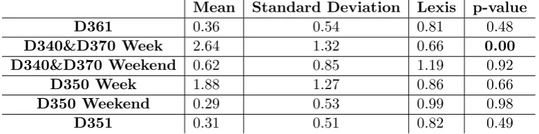
Mean Standard Deviation Lexis p-value

D361 0.36 0.54 0.81 0.48

D340&D370 Week 2.64 1.32 0.66 0.00

D340&D370 Weekend 0.62 0.85 1.19 0.92

D350 Week 1.88 1.27 0.86 0.66

D350 Weekend 0.29 0.53 0.99 0.98

[image:30.595.133.523.328.425.2]

D351 0.31 0.51 0.82 0.49

Table 2.1.: Summary statistics of the arrivals of elective patients, year 2017.

With respect to the elective patients, we see that the lexis ratio varies between 0.81 and 1.19. The Poisson distribution “passes” theχ2 test for all wards except the arrivals for the D340&D370 ward. However, by visual inspection of the observation vs. the Poisson fit we see that the variance is over all well captured by the Poisson fit. Especially in large samples, the H1 is quite easily accepted (i.e., not much deviation is required).

Combining the above, we conclude that a Poisson distribution is an appropriate fit for all wards. The summary statistics w.r.t. emergency patients are given in Table 2.2.

Mean Standard Deviation Lexis p-value

D361 1.87 1.31 0.92 0.74

D340&D370 1.69 1.56 1.43 0.00

D350 1.02 1.00 0.98 0.81

D351 0.80 0.85 0.90 0.52

Table 2.2.: Summary statistics of the arrivals of emergency patients, year 2017.

[image:30.595.155.496.584.653.2]

(31)

2.3. Arrivals

With respect to the emergency arrivals, the Poisson model provides a good fit for all wards except the D340& D370 ward (like in the elective case). By visual inspection we see that especially the frequency of days with 0 elective patients is “too high”. How-ever, especially for emergency arrivals, the Poisson process assumptions oftentimes hold. Moreover, again the variance of the observations is well captured by the Poisson model. Therefore, albeit the fact that the fit is not perfect, we still assume a Poisson distribution for this ward. Hence the overall conclusion is that the Poisson distribution provides a suitable fit for all wards regarding emergency arrivals.

2.3.3. Weekly Patterns

Elective Patients

The previous analysis gives the underlying distribution for the arrivals per day. It could be that this pattern is suitable for all days of the week. However, it could very well be the case that certain patients do not arrive during certain days. One can think of the absence of planned patients during weekends. This subsection serves to investigate this. In Figure 2.4 the number of elective arrivals in the year 2017 can be found per day for the wards D340 & D370 and D350.

Figure 2.4.: Weekly pattern of elective patients for the clinical wards D340& D370, and D350 in 2017. Data retrieved from data cube, n=729 and n=500 respectively.

The first thing that strikes is the significantly lower number of elective admissions during weekends on the clinical wards. This is perfectly in line with the expectations of the management that planned patients are not admitted during weekends. Besides that, it underpins the choice to split week from weekend days in the previous subsection.For the D350 ward (the surgical ward), we see furthermore that there is a peak on Friday and a trough on Mondays. This is confirmed by the fact that surgeries need some preparation which is not currently done during the weekend (hence the trough on Monday), and that scheduled admissions during the weekend should be prevented (hence the peak on Friday).

(32)

[image:32.595.123.573.482.623.2]

and troughs for the MCUs, these are not easily explained by the management. Further-more it should be noted that the total number of elective admissions on these wards is much lower than on the clinical wards, making it more likely that these peaks and troughs are just caused by randomness.

Figure 2.5.: Weekly pattern elective patients for the MCUs D351 and D361 in 2017.

Data retrieved from data cube, n=48 for both wards.

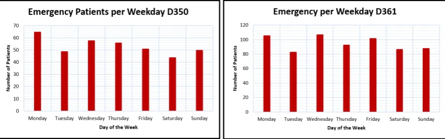
Emergency Patients

The same analysis is made for emergency patients. There is no reason to assume that there is such a pattern as with elective patients, because there is no reason to think that there are e.g., fewer stroke cases during weekends. This absence of a pattern is confirmed by the data of all wards. The emergency arrivals per weekday for one of the clinical wards and one MCU are pictured in Figure 2.6. For the other clinical ward and MCU the graphs can be found in the Appendix D and these show similar results.

Figure 2.6.: Weekly pattern emergency patients for D350 ward and D361 MCU in 2017.

Data retrieved from data cube, n=373 and n=666 respectively.

(33)

2.3. Arrivals

Conclusion

Both the data and the management tell us that there is a strong indication for a different number of arrivals per weekday for the clinical wards D340&D370 and D350. For the MCUs this is less obvious, and due to the low number of elective arrivals it is hard to draw inferences about this. A summary of the variation in the number of elective arrivals per weekday is given in Figure 2.7.

Figure 2.7.: Distribution of elective admissions per day of the week in 2017.

Using this section’s analysis and the Poisson assumption of Subsection 2.3.1, the arrival rates per day of the week for each ward are given in Table 2.3.

Monday Tuesday Wednesday Thursday Friday Saturday Sunday

D350 2.76 3.08 2.63 3.04 3.30 1.02 1.34

D340&D370 4.32 3.82 5.04 4.47 4.17 2.04 2.20

D351 1.21 1.11 1.11 1.15 1.32 1.06 0.84

D361 2.25 2.06 2.35 2.41 2.59 1.87 1.91

Table 2.3.: Poisson arrival rates per day of the week per ward, including both elective and emergency admissions. Data from 2017, retrieved from data cube, n=3219.

2.3.4. Arrivals per hour

Elective Patients

(34)

Emergency Patients

For emergency arrivals a similar analysis has been made. Although the differences throughout the day are less significant, there still is some pattern. The number low-est number of patients arrive around 08:00 AM. This number is slowly increasing with midnight as peak hour. After that, the numbers are decreasing again till sunrise. This is not counter intuitive because e.g., when a patient has a stroke, he or she could remark this by not being able to move certain extremities when he or she wakes up (and thus not during the night). There are some strange peaks for some wards around midnight. The management has explained that when the nursing staff starts the night shift around 11:00 PM, they first evaluate the evening shift with the evening nurses. After that, they meet with patients, provide them their medicine etc. When most patients sleep and the nurses got some spare time (around 01:00 AM) they update the admissions of the last two hours. This could cause a peak around 01:00 AM, whereas the admissions are actu-ally spread out more evenly. This tend to happen more with emergency patients, due to their unexpected arrival. The same phenomenon happens in the morning and afternoon. The graphs picturing the hourly emergency arrivals can be found in Appendix E.

Figure 2.8.: Hourly admissions of elective patients in 2017. Data retrieved from data cube, n=503 and n=48 respectively

Figure 2.9.: Hourly admissions of elective patients in 2017. Data retrieved from data cube, n=729 and n=48 respectively

(35)

2.3. Arrivals

Conclusion

Both the elective and emergency admissions do show a difference throughout the day. To quantify this, a heat map has been made which is pictured in Figure 2.10. This

Figure 2.10.: Distribution of elective and emergency arrivals per hour of the day in 2017.

heat map can be used to determine the busy moments on a day, i.e., the moments with a lot of admissions. This is of course useful for answering the main question of this research, but can also help with e.g., nurse scheduling. Emergency patients tend to arrive between 1:00 PM and 10:00 PM, with a concentration around 6:00 PM. Elective patients arrive roughly between 7:00 AM and 1:00 PM. The hourly variability discovered in this subsection has to be taken into account in our model which will be introduced in Chapter 4. Therefore, we already give the arrival rates incorporating the hourly variability (i.e., a slight adaptation of the ones given in Table 2.3). Since giving hourly arrival rates will result in 168 different rates per ward which is a bit cumbersome, we assume equal emergency arrivals over the day. Furthermore we assume that all elective patients arrive equally distributed over daytime hours, and are forbidden during night. This somehow represents reality. Not taking into account hourly variability in detail might seem an unrealistic simplification, but this will be justified in Chapter 5 in Section 5.1. The adapted arrival rates are given in Table 2.4.

D N D N D N D N D N D N D N

D340&

D370 7.15 1.48 6.37 1.27 8.21 1.87 7.23 1.71 6.03 2.31 2.58 1.50 2.89 1.51 D350 4.27 1.25 5.20 0.96 4.12 1.14 5.00 1.08 5.62 0.98 1.19 0.85 1.74 0.94

D351 1.51 0.91 1.52 0.70 1.44 0.77 1.37 0.93 1.80 0.84 1.32 0.80 0.40 0.64

D361 2.41 2.08 2.48 1.63 2.60 2.10 3.01 1.82 3.18 2.00 2.04 1.71 3.45 2.76

Table 2.4.: Daily Poisson arrival rates (both elective and emergency) split up into day (D) and night (N). Retrieved from data cube, year 2017, n=3219.

2.3.5. Arrivals throughout the year

(36)

holidays. In Figure 2.11 the admissions for the entire department have been pictured for both emergency and elective arrivals. The choice to display the entire division at once instead of splitting into wards is made deliberately because it is not expected that this will differ considerably per ward.

Figure 2.11.: Arrivals of respectively emergency and elective patients within the N&N department in 2017. Data retrieved from data cube, n=1903 and n=1328 respectively.

As can be seen there are no major differences throughout the year for emergency arrivals; we see that the number of admissions in January is much lower than e.g., in October. There is no clear explanation for this. For elective arrivals however, we see that the number of admissions is a bit lower during the months April and July. For April, this can be explained by the large number of holidays within this month. For July this can be explained because this is a typical month that people go on vacation.

2.4. Length of Stay

2.4.1. Gini Coefficient

The length of stay is defined as the time that a patient occupies a bed (see Subsection 2.2.1). As a Poisson distribution is a distribution often used to model customer arrivals, there are also distributions that are often used for modelling service times (the LOS can be regarded as such). One can think of the Gamma, Weibull and Lognormal distribution (Law, 2015:286-305). The LOS distribution is analysed per ward. Contrary to the arrivals, there is no clear pattern in this data. This unfortunately was the case for all wards. Several distributions have been tried, but none of them provided a reasonable fit. This is underpinned by analysis of e.g., De Bruin et al. (2009) and Costa et al (2003). Most likely this “fuzzy” data is caused by the fact that the LOS should not be considered as being equally distributed for all patients. We present several summary statistics for all wards. In addition to the regular summary statistics, we also present the Gini coefficient (Gini, 1912). This is suggested by De Bruin et al. (2009), and based on the Lorentz curve often used in economics. The Lorenz curve can be used to picture the

(37)

2.4. Length of Stay

concentration of wealth (Lorenz, 1905) (i.e., what percentage of the total wealth belongs to what percentage of the population). See Figure 2.12 for an example.

Figure 2.12.: A Lorenz curve.

The bigger the “belly” i.e., area A, the more unevenly wealth is distributed. The blue line means perfect equality. The Gini-coefficient (G) quantifies this dispersion as:

G= A A+B

Now this idea can be used to analyse the LOS. If the distribution of the LOS would be equal for all patients, G would be close to 0 (i.e., there would be no “belly” at all because of perfect equality). If G is close to one there is a lot of dispersion and the distribution is more variable. It is expected that for some wardsGwill be quite close to 1, the difference between the medians and means is big. This means that a small part of the patient population has a disproportional long LOS. For the calculation of G per ward, we use the formula provided by De Bruin et al. (2009):

G= 1

n(n+ 1−2

Pn

i=1(n+ 1−i)yi

Pn

i=1yi

) (2.7)

With n being the total number of observations (i.e., registered LOS), yi the LOS of

(38)

2.4.2. Summary Statistics

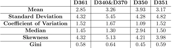
The summary statistic per ward w.r.t. the LOS are given in Table 2.5.

D361 D340&D370 D350 D351

Mean 2.85 3.26 3.93 3.17

Standard Deviation 4.32 5.45 4.28 4.82

Coefficient of Variation 1.52 1.67 1.09 1.52

Median 1.45 1.30 2.94 1.50

Skewness 4.32 5.13 4.21 3.98

[image:38.595.157.499.131.227.2]

Gini 0.58 0.64 0.45 0.59

Table 2.5.: Summary statistics LOS in 2017. Retrieved from data cube, n=3226.

As can be seen, patients on average stay the longest on the D350 (surgical) ward, and the shortest on the D361 MCU. The LOS data does not really have a pattern which is, as explained before, most likely caused by different LOS distributions for different patient groups. Striking are the big differences between the means and medians. This could indicate very skewed data or outliers. The latter cannot be easily confirmed since for instance on the D340&D370 ward there are many patients who stay very short, and many patients who stay much longer. This also explains the large standard deviations. The best thing to do would be splitting to search for the underlying patient groups having a homogeneous distributions.

2.4.3. Distribution Fitting

As said, the LOS data is not as easily described by a probability distribution as the arrival data. This is also encountered by other studies, see for example De Bruin et al. (2009) or Costa et al. (2003). Following the reasoning of Subsection 2.4.1 and our intuition, it might very well be the case the group of patients should be split into patients who stay long and short, each having their own distribution. According to Adan and Resing, we should fit a hyper exponential distribution with two exponentials if the coefficient of variation is greater than or equal to 1 (2015:17). This happens to be the case for all wards (see Table 2.5). The hyperexponential distribution sums several exponential distributions, each with a different parameter (see Appendix B.3). This corresponds to our intuition because e.g., the long stay patients could have their “own” exponential distribution as do the short stay patients. For a hyperexponentially distributed variable the notation Hk(p1, ..., pk;µ1, .., µk) is common. In this notation, k is the number of

groups, pi stands for the proportion (size) of group i and µi for the parameter of the

exponential distribution of groupi (i.e., the ALOS of group iis _µi1). In order to apply this distribution to our case, we must estimate the parametersp1, p2, µ1 andµ2 (k= 2).

Oftentimes, we assume equal weighted means for both subgroups, i.e., p1 µ1 =

p2

µ2

(“bal-anced means assumption”). Furthermore, since we divide the total population into subgroups according to a proportion pi we have p1+p2 = 1 and _µp1₁ +_µp2₂ = ALOS. It

turns out that the Gini coefficientGcan be of help in this matter. De Bruin and Bekker

(39)

2.4. Length of Stay

(2010) indicate that when 0.5 ≤ G ≤ 0.75 we can estimate the parameters using the Gini coefficient as follows:

b

p1=

1 2 −

r

G−1

2 µˆ1 =

ALOS 2 ˆp1

(2.8)

b

p2= 1−pˆ1 µˆ2 =

ˆ p2µˆ1

ˆ p1

This applies to three out of four wards (see Table 2.5). For the other ward, we need some additional analysis provided by Adan and Resing (2015:18). If G does not fulfill the requirement of De Bruin and Bekker (2010), we can estimate the parameters with:

ˆ p1=

1 2 1 + s b

cv2−1

b

cv2+ 1

ˆ µ1 =

ALOS 2 ˆp1

(2.9)

ˆ

p2= 1−pˆ1 µˆ2 =

ˆ p2µˆ1

ˆ p1

Where cv_b = s

X denotes the coefficient of variation. The results are given in Table 2.6,

together with the p-value of the χ2 goodness-of-fit test.

D361 D340&D370 D350 D351

ˆ

p1 0.79 0.88 0.65 0.80

ˆ

p2 0.21 0.12 0.36 0.20

1 ˆ

µ1 1.81 1.85 3.05 1.99

1 ˆ

µ2 6.78 13.46 5.54 7.80

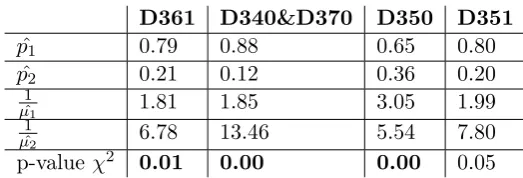
[image:39.595.135.397.376.465.2]

p-value χ2 0.01 0.00 0.00 0.05

Table 2.6.: Results of fitting the hyperexponential distribution to the LOS of the four wards.

(40)

[image:40.595.118.566.84.226.2]

Figure 2.13.: LOS 2017 data vs. hyperexponential distribution. Note: LOS over 20 days have been left out for illustratory purposes. Data retrieved from data cube, n=714 and n=1345.

2.5. Performance

This section evaluates the current performance with respect to the defined KPIs. The KPI Length of Stay will not be considered again, since it has been extensively analysed in the previous section. First, we discuss the bed occupancy, and after that the rejection rate.

2.5.1. Bed Occupancy

To evaluate the current performance with respect to bed occupancy, Equation 2.6 is used. The input needed for Equation 2.6 is given in Sections 2.3 and 2.4. Besides Little’s Law, we also calculated the bed occupancy using the hourly presence data (note again, this data is very sensitive for input errors). In Table 2.7 the average bed occupancy for the year 2017 is given, using both Equation 2.6 and 2.4.

Little’s Law Data

D340&D370 66.67% 69.38%

D350 79.03% 82.98%

D351 58.87% 51.64%

D361 90.73% 82.20%

Table 2.7.: Bed occupancy per ward in 2017.

First of all, the bed occupancy for both the D361 and D350 ward are much higher compared to the other wards. Together with the variable arrival- and LOS process, this results in a relatively high rejection rate (see Table 2.8). Little’s Law and the data pretty much coincide for the clinical wards, but differ a bit for the MCUs. Especially for the MCUs (a lot of) data was missing, what could have caused this result. See Chapter 6

[image:40.595.226.429.503.575.2]

(41)

2.5. Performance

for a thorough discussion about the available data. Although controversial (see Chapter 4), the management strives for a bed occupancy of 85% for all wards.

2.5.2. Diverted Patients

As discussed in Section 2.1.3, diverted patients are patients that are assigned to a bed on another ward other than the ward where he belongs. In the worst case, a patient is diverted to another division or even hospital but this rarely happens. Ideally we would prefer to know the frequency of this phenomenon (for instance to be able to say something about the true arrivals of a ward) , but the data cube does not provide the required data. This complicates using this Chapter’s analysis for mathematical models since the measured admissions do include diverted patients from other wards. Since for the MCUs diversions almost exclusively happens between the MCUs (i.e., not to other divisions or hospitals) this is not a problem because these wards are merged. For the clinical wards this is more troublesome since there is also a third clinical within the division ward (D360) to which patients can be diverted. However, this ward is left out of consideration in this thesis. Due to the lack of data, we assume that all patients diverted from one of our clinical wards (e.g., D350) are placed on the other (e.g., D340&D370) and v.v, cf. Section 5.1.

2.5.3. Rejection Rate

The rejection rate can be calculated using Equation 2.3. Unfortunately, there is no data available about the number of rejections. One could think of considering the fraction of time that the wards are fully occupied considering the same data used for calculating the bed occupancy. However, this data is as stated before highly sensitive for input errors (e.g., more patients than beds present). Another way of calculating the current rejection rate is by considering the queueing model suggested in Chapter 5, which also is used for the calculation of the future situation (see Chapter 3). Because of the sensitivity to input errors we decided to use the model to estimate current performance. The results are depicted in Table 2.8.

Model D340&D370 3.4%

D350 10.9%

D351 7.5%

[image:41.595.204.331.529.600.2]

D361 23.5%

Table 2.8.: Estimations of current rejection rate, calculated using the data (first column) and the model of Ch. 5 (second column).

(42)

2.6. Conclusion

This chapter serves to answer the first and second research question. The relevant KPIs are the bed occupancy, the LOS and the rejection rate. Since the data available is erroneous (see Chapter 6) we decided to calculate the current bed occupancy using Little’s Law and the current rejection rate using the model of Chapter 5. The current bed occupancy for the clinical wards is 69.38% (D340&D370) and 82.98% (D350). For the MCUs, the current occupancy is 51.64% (D351) and 82.20% (D361). The current rejection rates for the clinical wards are 3.4% (D340&D370) and 10.9% (D350). For the MCUs, the rejection rates are 7.5% (D351) and 23.5% (D361). The management now primarily bases bed capacity decisions on a target occupancy of 85%. Besides that this target is not met, many studies show that bed capacity decisions should rather be based on the rejection rate. The target rejection rates for the new clinical ward and MCU are 5% and 3% respectively.

For modelling purposes, we wanted to find a suitable distribution for the LOS data and to discover the underlying arrival pattern. The LOS data is known to be difficult, since there are different subgroups within the patient population with different LOS dis-tributions (e.g., short and long stay patients). We fitted a hyperexponential distribution to the LOS data for all wards, which sums various exponential distributions and thus copes with the different subgroups. The ALOS in 2017 was around 3 days for all wards. The arrival data turned out to be well approximated by a non-stationary piecewise con-stant Poisson process with a cycle length of 1 week. The rates change each day part of 12 hours (i.e., day and night).

(43)

3. Analysis of the New Situation

Introduction

As explained in Section 1.3.2 we are primarily interested in the number of beds on the clinical ward and MCU after the merger. The analysis in Chapter 2 shed light on the current situation, and can be used to compare with the estimations of the performance of the future situation. This chapter serves to answer the third research question, and has roughly the same set up as the aforementioned chapter. First, the arrival process is discussed, and thereafter the LOS is examined.

3.1. Physical Changes

As discussed, the merger will result in both clinical wards and MCUs being combined into one clinical ward and one MCU respectively. The management hopes to gain economies of scale and to improve the communication between the medical professionals. The merger will eliminate the flow in between the clinical wards and MCUs, since the clinical wards and MCUs are no longer separated. This results in a lower arrival rate and higher LOS. The former is caused by the absence of transfers, and the latter by the transfer patients now stay on a single ward. Figure 3.1 illustrates the physical change.

3.2. General approach

(44)

3. Analysis of the New Situation

Figure 3.1.: A schematic view of the current and future situation.

We thus assume independency of the arrivals for both clinical wards and MCUs.

3.3. Arrivals

The arrival process will again be analysed for the clinical ward and MCU separately. First, we look at the arrivals per day. Subsequently patterns throughout the day and week respectively are investigated. As shown in Section 2.3, the arrival processes for all wards tend to be well described by a (non-stationary) Poisson process. One of the properties of a Poisson process is the merging property: if we have two independent Poisson processes X and Y with parameters λ1 and λ2 respectively, we can describe

the joined process Z = X+Y again with a Poisson process, with parameter λ1+λ2.

This directly applies to our situation, since we have just assumed an independent arrival process for the separate wards. Using the merging property, the arrival rates for the new wards are given in Table 3.1.

D N D N D N D N D N D N D N

CW 7.15 1.48 6.37 1.27 8.21 1.87 7.23 1.71 6.03 2.31 2.58 1.50 2.89 1.51

[image:44.595.200.456.84.297.2]

MCU 4.27 1.25 5.20 0.96 4.12 1.14 5.00 1.08 5.62 0.98 1.19 0.85 1.74 0.94

Table 3.1.: Predicted Poisson arrival rates for the new clinical ward and MCU per day of the week, split into day (D) and night (N) time.

(45)

3.4. Length of Stay

Similar to the current situation, we also analyse the LOS for the future situation. We generated the LOS data for the new wards as described in the section “General Ap-proach”. The summary statistics for the LOS data of the new wards can be found in Table 3.2. For modelling purposes we again have fitted a statistical distribution through the data. For both wards again a hyperexponential seems to describe the underlying data properly and is therefore assumed to be a good fit. The parameters of both hy-perexponential distributions together with the p-values of theχ2 goodness-of-fit test are given in Table 3.2. Note that the p-values suggest a bad fit. However, because the variability of the LOS data is well captured and taking into account that it is hard to find a suitable distribution for the LOS data, we ignore this.

CW MCU

Mean 3.52 2.94

Standard Deviation 5.03 4.47

Coefficient of Variation 1.43 1.52

Median 2.10 1.45

Skewness 4.92 4.21

Gini 0.57 0.59

ˆ

p1 0.77 0.79

ˆ

p2 0.23 0.21 1

ˆ

µ1 2.29 1.86

1 ˆ

µ2 7.69 7.10

[image:45.595.159.375.255.425.2]

p-value χ2 0.00 0.02

Table 3.2.: Summary statistics and parameter estimation of the LOS of new clinical ward and MCU.

3.5. Conclusion

(46)

(47)

4. Modelling Approach

This chapter discusses the modelling approaches available to answer the central research question, and to provide argumentation to make a valid choice amongst them. This chapter is supported by the existing literature on the subject. Therefore we first define the theoretical perspective used for the literature search. Subsequently we provide an overview of the techniques available to determine the number of beds, and conclude with the method of our choice.

4.1. Theoretical Perspective

The theoretical perspective used in this chapter is that of optimizing hospital bed ca-pacity along the edges of Operations Research (OR). Optimizing in this context means establishing a perfect trade off between bed occupancy and patient rejections (cf. Sec-tion 2.2), while keeping the variability in bed demand in mind. OperaSec-tions Research is an umbrella term consisting of mathematical techniques to support decision making.

4.2. General notions

(48)

4. Modelling Approach

4.3. Queueing Theory

Queueing theory is a branch of OR and can be used to describe and predict behavior of waiting lines. It also entails the study of the arrival process (input process) and the service process (output process). In case of a hospital ward, the beds can be seen as servers, the patients’ length of stay as service time, the admission of patients per time as arrival rates and a possible waiting list as queue. Queueing systems are oftentimes categorized using the Kendall-Lee notation : A/S/c/K/N/D (Kendall,1951). In this notation, A stands for the arrival process, S for the service process, c for the number of servers, K for the queue capacity, N for the population size and D for queueing discipline. Oftentimes the last two symbols are omitted, because of their irrelevance to the system on hand.

Regarding the problem under examination, several queueing related methods are pro-posed. Green (2002) and Cochran and Roche (2008) suggest theM/M/c/∞ system to model the situation. This model assumes exponentially distributed inter arrival times (i.e., a Poisson process, see Subsection 2.3.1), exponentially distributed service times, c servers (beds) and an infinite queue capacity. Exponentially distributed inter arrival times are proposed for both elective and scheduled admissions. As discussed before, it is reasonable to approximate both scheduled and unscheduled arrivals with a Poisson process. Since two merged Poisson processes again form a Poisson process, the “M” as-sumption for patient arrivals is not unreasonable on itself, but it also assumes stationary. As is pointed out in Chapter 2, the arrival process for elective patients varies across the week. The model its main advantage is the relatively simple calculations of KPIs. It is not hard to point out the restrictions of this model. For instance, this model assumes infinite queue capacity. It is probably more realistic to assume a finite queue capacity, or even no queue capacity at all since patients that arrive when all beds are occupied, are diverted to another ward. Besides that, the model assumes homogeneous LOS and arrival rates, which might very well be a wrong assumption as is pointed out in Section 2.6.2. Green (2002) does consider the refusal of patients, by examining the probability of delay. Cochran and Roche (2008) optimize capacity with respect to target utilization, which is not the way to go as explained earlier.

De Bruin et al.(2009) model a hospital ward as a M/G/c/c queueing system (also known as Erlang-Loss model). In this model, the patient arrival process is assumed to be a Poisson process, the service distribution is not pre-specified (G means general) and that the number of beds equals the queue capacity i.e., patients that arrive when all beds are occupied are “blocked”. According the De Bruin et al., blocked in this context could mean sent away to another ward, or even another hospital. This seems to be a more accurate approach, because in our situation there also is no waiting room and the LOS distribution is hard to specify. A drawback is that also this model does not take non stationarity of the arrival process into account. Besides that, there is still some generalization of the LOS needed, albeit to a lesser extent than the previous approach.

Gorunescu et al.(2002) and Belciug and Gorunescu (2014) provide an even more so-phisticated approach because they also take several cost aspects into consideration. The method is based on theM/P H/c/c model. This model is identical to the one De Bruin