Asymmetric and Non atmospheric Consumption Externalities, and Efficient Consumption Taxation

Munich Personal RePEc Archive

Asymmetric and Non-atmospheric

Consumption Externalities, and Efficient

Consumption Taxation

Eckerstorfer, Paul and Wendner, Ronald

University of Linz, Austria, University of Graz, Austria

17 January 2013

Online at

https://mpra.ub.uni-muenchen.de/45521/

Asymmetric and Non-atmospheric Consumption

Externalities, and Efficient Consumption Taxation

⋆

Paul Eckerstorfer

and Ronald Wendner

a Department of Economics, University of Linz, Austria b Department of Economics, University of Graz, Austria

January 16, 2013

Abstract. We analyze the effects of a generalized class of negative consump-tion externalities (asymmetric and non-atmospheric) on the structure of efficient commodity tax programs. Households are not only concerned about consumption reference levels — that is, they gain utility from “keeping up with the Joneses” — they also exhibit altruism. Two sets of efficient tax regimes are compared, based, on a welfarist- and a non-welfarist optimality criterion, respectively. Altruism turns out not to be at odds with the consumption externalities. Rather, altruism impli-cates a bound on efficient utility allocations. A non-welfarist government tolerates less inequality than a welfarist one. In the welfarist (non-welfarist) case, first-best personalized commodity tax rates respond highly sensitively (barely) to whether or not a consumption externality is asymmetric or non-atmospheric. If personalized commodity tax rates are not available (second-best case), the tax rate on a non-positional good is typically different from zero for corrective reasons. For plausible functional forms and parameter values, numerical simulations suggest that second-best tax rates are rather insensitive with respect to both the optimality criterion and the “nature” of the consumption externality.

Keywords and Phrases: Consumption externality, keeping up with the Jone-ses, optimal (commodity) taxation, genuine altruism, non-welfarist government.

JEL Classification Numbers: D62, H21, H23

⋆_{We thank Johann K. Brunner and Susanne Pech for significant comments on a previous draft.}

However, we retain sole responsibility for any remaining errors.

Since ... appearance tyrannizes over truth and is lord of happiness, to appearance I must devote myself.

. — Plato, The Republic (Book II)

1

Introduction

This paper addresses the effects of a generalized class ofnegative consumption exter-nalities (asymmetric and non-atmospheric) on the structure of efficient commodity taxation in a framework with both a positional and a non-positional commodity. That is, individual utility isnot independent of other individuals’ consumption. In fact, households form consumption reference levels, a fact well established in the literature (cf. the discussion below). Consumption reference levels give rise to a consumption externality. This externality is often referred to as a keeping up with the Joneses externality.1

In contrast to the prior literature, the present analysis takes three important facts into account. First, some people typically contribute more to a consumption reference level than others. In this case, we refer to the consumption externality

as a non-atmospheric one. In other words, not every household belongs to one’s

consumption reference group (to the same degree).2 _{In contrast, a consumption}

ex-ternality is termedatmospheric if consumption of the positional commodity of any two households are perfect substitutes regarding the generation of one’s consump-tion reference level. Second, consider the reference groups of two given households. Consumption of a member of both reference groups may exert different (asymmet-ric) effects on these two household’s consumption reference levels — a situation we refer to as an asymmetric consumption externality. Third, households are not only concerned about consumption reference levels, they also exhibit altruism (cf. Johansson 1997).

This paper is motivated by the recent literature on consumption externalities and happiness. Psychologists and behavioral economists have established that

indi-1

Different authors employ various terms, with slightly varying meanings. These terms in-clude(negative) consumption externality,positional-, status-, relative consumption,jealousy,envy,

catching up with the Joneses. As made precise below, we focus on the case of keeping up with the Joneses in this paper.

2

viduals experience happiness by doing well relative to some reference group (Brekke and Howarth 2002, Easterlin 1995, Frank 1985, 1999). Important survey experi-mental studies substantiating this evidence include Johansson-Stenman et al. (2002, 2006), and Solnick and Hemenway (1998, 2005).3 _{The main response of economic}

theory to this evidence has regularly consisted in allowing for a uniform consump-tion reference term — commonly the economy’s average consumpconsump-tion — in the utility functions of households. While consideration of the consumption reference level in an otherwise standard framework has delivered important insights4_{, the}

usual specification of “the” reference level still exhibits two major shortcomings. The first shortcoming refers to a household’s reference group(s). There may be different reference groups, and even within a reference group, some individuals may be considered more influential than others. For example, Cowan et al. (2004) argue that some activities become more desirable when they can be shared with a group of peers (peer group effect). Other activities become more desirable if they allow the consumer to emulate the consumption of an elite group that he or she aspires to join (aspiration effect). Still other activities become more desirable when the individual can, through wealth or personal endowments, out-shine its peers (distinction effect). In the jargon adopted in this paper, within a reference group, a household may be more concerned with some individuals rather than with others. That is, a consumption externality is usually non-atmospheric. In addition, the consumption of a given household might matter more for some individuals than for others, that is, a consumption externality commonly is asymmetric. Put differently, even if two households are concerned with thesame reference group, this does not imply that these households also share the same consumption reference level.

The second shortcoming refers to the fact that households not only care about consumption reference levels but also about inequality or redistribution (Brekke and Howarth 2002). As has been shown, individuals dislike being “too different” from their peers. Fehr and Schmidt (1999), find that people dislike income inequality,

3

A large number of further empirical studies add significant evidence. Cf. Alpizar et al. (2005), Alvarez-Cuadrado et al. (2012), Carlsson et al. (2007), Ferrer-i-Carbonell (2005), Luttmer (2005), Maurer et al. (2008), McBride (2001), Neumark et al. (1998), and Ravina (2007).

4

but they are more upset when their own income falls short than they are pleased by an excess in comparison to their reference levels.

In this paper, we take both of these shortcomings into account for the derivation of efficient tax programs under both a welfarist and a non-welfarist government. A welfarist government fully respects individual preferences in the formulation of the welfare criterion. On the other hand, a non-welfarist government does not tolerate status preferences — those are basically a form of envy — to be part of the welfare criterion.5 _{That is, in the non-welfarist case the government’s and individuals’}

preferences differ. Our analysis sheds light on the optimal policies that emerge from these two different welfare criteria.

This paper is related to the prior literature on optimal taxation and consumption externalities (see, e.g., Aronsson and Johansson-Stenman 2008 and 2010, Boskin and Sheshinski 1978, Layard 1980, Ljungqvist and Uhlig 2000). From this literature it is well established that an externality due to relative consumption concerns calls for some corrective element in the tax system. For example, Aronsson and Johansson-Stenman (2008) show that the presence of a keeping up with the Joneses externality implies substantially higher marginal income tax rates. The issue of a consumption externality being non-atmospheric rather than atmospheric has also already been taken up by Eckerstorfer (2013), Micheletto (2008) and Wendner (2013). From these studies it has become evident that the nature of a consumption externality indeed matters for the optimal tax structure. However, this literature does not consider asymmetric consumption externalities. Our paper is also related to the literature that studies optimal tax policy from the perspective of a non-welfarist government (see, e.g., Besley 1988, Blomquist and Micheletto 2006, O’Donoghue and Rabin 2006). These studies are concerned with the taxation of sin goods and (de)merit goods where the government does not fully respect households’ preferences.

This paper explicates four results. First, efficient welfarist first-best tax rates on the positional good are personalized and directly depend on the specific features of the non-atmospheric and asymmetric consumption externality. Specifically, house-holds contributing more than others to the generation of the consumption exter-nality face a higher first-best tax rate. However, in the non-welfarist case, efficient first-best tax rates directly depend on the specific features of the consumption

exter-5

nality only if the consumption reference level does have an impact on the marginal rate of substitution of the positional good for leisure. Second, if the consump-tion externality is non-atmospheric, the efficient corrective second-best tax rate on the non-positional good is generally different from zero, once a personalized tax on the positional good is not available. Third numerical simulations reveal that the first-best tax rates are highly sensitive with respect to the specific features of the consumption externality. In contrast, the second-best tax rates barely respond to the specific features of the consumption externality. Moreover, the second-best corrective tax rate on the non-positional good turns out to be quite low. Fourth, altruism and keeping up with the Joneses preferences are not contrasting motives — even if the consumption externality is non-atmospheric or asymmetric. Rather, altruism requires the distribution of utility not to bee too unequal, in a well-defined sense. It imposes a fairness condition which narrows the set of efficient allocations to those that are not too distant from an egalitarian allocation. The specific set of fair allocations is strongly affected by the features of the consumption externality. More inequality is tolerated towards households contributing more than others to the generation of the consumption externality. Moreover, for a given consumption externality, the set of fair allocations under a non-welfarist government is smaller than that under a welfarist government. A non-welfarist government tolerates less inequality compared to a welfarist government.

To sum up, the nature (non-atmospheric, asymmetric) of the consumption ex-ternality exhibits a strong impact on first-best commodity tax rates as well as on fair efficient utility allocations. While this is potentially also true in the second-best, numerical simulations reveal that second-best tax rates are rather insensitive with respect to both the optimality criterion and the “nature” of the consump-tion externality. Altruism has no offsetting effect on the corrective elements in the tax system induced by the presence of status effects. However, altruism implies a fairness condition which requires the efficient distribution of utility not to be too unequal.

impact of altruism on “fair” (utility) allocations. Section 4 considers efficient first-and second-best tax programs under a non-welfarist government. The efficient tax rates differ between the welfarist- and non-welfarist optimality criteria. Therefore, Section 5 presents numerical simulations in order to give a rough indication of the magnitude of the differences in efficient tax rates between the welfarist- and non-welfarist cases. Section 6 concludes the paper. The appendix contains proofs and mathematical results that support the analysis of the main text.

2

The model

We consider a static economy with n households. A household i ∈ N = {1, ..., n}

has preferences over two private goodsxi and zi, leisureli and a reference

consump-tion level zi. In addition, households derive utility from the average utility of all

households in the economy. We consider spending on x as a nonpositional form of consumption and spending on z as status consumption, i.e. for goodz households care about their relative consumption with respect to others. Households differ in their exogenous earning ability wi and in their preferences. The preferences of a

household are represented by the concave utility function

ui(xi, zi, li, zi) +

ϕ n

n

X

j=1

uj(xj, zj, lj, zj), (1)

where ϕ ≥ 0 is a weighting factor which is assumed to be constant across house-holds. Utility of a householdiincreases in own private consumption and leisure and decreases in the reference levelzi. Further, similarly to Brekke and Howarth (2002)

utility of a household increases with the average utility of the whole population, i.e. households are altruistic as they also derive satisfaction from the general welfare in the economy.6 _{The strength of altruism is reflected by ϕ. Both the reference}

level and the average utility of all households are considered to be exogenous by a household.7

The consumption reference level zi gives rise to a negative consumption

exter-nality. In this paper, we focus on the case of a keeping up with the Joneses (KUJ-) externality. Dupor and Liu (2003) define preferences exhibiting a KUJ externality

6

Johansson (1997) refers to this form of altruism asgenuine altruism. 7

by ∂(uz/ul)/∂z > 0.8 That is, we assume that the marginal utility of consuming

the status good relative to that of leisure increases in the reference level.

Let the reference level of a household i concerning consumption of good z be determined by

zi =

1

n

n

X

j=1

aijzj. (2)

with i, j ∈ N. The nonnegative coefficient aij indicates the amount by which

the consumption of one unit of the status good, z, by the externality-generating household j raises the consumption reference level of householdi. Thus, regarding the composition ofzi, thesecond index of coefficients aij refers to the household of

origin of the consumption externality, and thefirst index of coefficientsaij refers to

the household of destination of the consumption externality. If aij = 1 for all i, j ∈

N the reference level is equal to the economy’s mean consumption of the status good. However, in general these weights differ between different households of origin (aij 6=

aij′ with i, j, j′ ∈ N and j 6= j′) and between different households of destination

(aij 6=ai′_j withi, i′, j ∈N andi6=i′). This gives rise to two forms of heterogeneities

in the reference level. First, if weights differ between households of origin a given consumption quantity of some households contributes more to the consumption reference levels than the same consumption quantity of other households. Second, if weights differ between households of destination, different households, in general, have different reference levels.

We say that an externality is of the atmospheric type if weights are constant across all households of origin. In contrast, if weights differ across households of origin, then the externality is said to be of thenon-atmospheric type.

Definition 1 (Non-atmospheric consumption externality)

An externality is said to be non-atmospheric if aij 6=aij′ for some i, j, j′ ∈N with

j 6=j′_{. Otherwise it is atmospheric.}

If an externality is non-atmospheric, the status consumption (zj, zj′) of households

j and j′ _{are not perfect substitutes regarding the generation of z}

i. Assume that

NH ⊂ N represents the set of all households with a “high” social status. If the

reference consumption levels depend only on the consumption of members of this

8

group, thenaij >0 if j ∈NH and aij = 0 if j /∈NH for all i∈N.

We say that an externality issymmetric if weights are constant across households of destination. In contrast, we say that an externality is asymmetric if weights differ between households of destination.

Definition 2 (Asymmetric consumption externality)

An externality is said to be asymmetric if aij 6=ai′_j for some i, i′, j ∈N withi6=i′.

Otherwise, it is symmetric.

As long as aij =ai′_j for all i, i′, j ∈N, z_i =z_i′. That is, as long as the externality

is symmetric, there is a unique reference level for the whole population. Only if the externality is asymmetric, households have different reference levels, no matter whether the externality is non-atmospheric or not:

Lemma 1 (Asymmetric and non-atmospheric consumption externality)

An asymmetric consumption externality implies personalized consumption reference levels, irrespective of whether the consumption externality is of the non-atmospheric type or not.

There is a linear technology for the production of private goods with labor as the only input. Quantities of goods are chosen such that the (constant) marginal costs of production are equal to one for all commodities. Given competitive markets, the producer prices of both commodities equal one and the wage rate of a household i

equals productivity wi. The time endowment of a household is normalized to one

and is divided between labor and leisure. Hence, the labor income of a household is given by wi(1−li).

2.1

The household’s maximization problem

In a first step, we characterize consumer behavior given competitive markets. House-holds maximize their utility subject to the private budget constraint

qxxi+qzzi ≤wi(1−li) +τi, (3)

whereqx = 1 +tx andqz = 1 +tz are consumer prices andτi is a lump-sum transfer.

and tz and a lump-sum element τi.9 Labor income is left untaxed without loss of

generality.

Households choose consumption and leisure such that the following necessary conditions hold:

−M RS_zxi = 1 +tz 1 +tx

, (4)

−M RS_lxi = wi 1 +tx

, (5)

with M RSkx ≡ −uk/ux and k ∈ {z, l}. Households choose x, z, l so as to equalize

their marginal rates of substitution to relative prices. Observe that the altruism parameter ϕ does not appear in these optimality conditions, i.e. the presence of altruism has no effect on the consumption and leisure decision of a household. A household’s indirect utility function is given by

vi(qx, qz, τi, zi) +

ϕ n

n

X

j=1

vj(qx, qz, τj, zj). (6)

It is the maximum utility a household i can obtain, given consumer prices, the lump-sum transfer and the reference level. Observe that due to the presence of altruism the indirect utility of household i also depends on the lump-sum element and reference level of all other households.

2.2

Characterization of a first-best allocation

In this subsection we characterize first-best allocations for this economy and analyze which tax instruments are required to implement these allocations. Assume that a social planner can directly determine xi, zi, li for each household i. Then a Pareto

efficient first-best allocation is a solution to the following problem:

max

xi,zi,li,zi,i=1,...,n

u1(x1, z1, l1, z1) + ϕ n

n

X

j=1

uj(xj, zj, lj, zj) (7)

9

subject to

ui(xi, zi, li, zi) +

ϕ n

n

X

j=1

uj(xj, zj, lj, zj)≥ui i= 2, ..., n (µF Bi ) (8)

n

X

i=1 xi+

n

X

i=1 zi =

n

X

i=1

wi(1−li) (λF B) (9)

zi =

1

n

n

X

j=1

aijzj i= 1, ..., n (γiF B) (10)

whereui is some minimum utility requirement for householdi. Lagrange multipliers

are given within parenthesis and the index FB refers to first-best. By varying the minimum utility requirement ui the family of Pareto efficient allocations can be

characterized. In the Appendix we show that for an interior solution the following conditions hold:

−M RS_zxi = 1 +

1

n

Pn

j=1γjF Baji

λF B

| {z }

Ψi

(11)

−M RS_lxi =wi (12)

1 +ϕ

ϕ ≥

1

n

n

X

j=1

∂ui/∂xi

∂uj/∂xj

(13)

for i = 1, ..., n. Equations (11) and (12) state conditions for an efficient allocation of consumption goods and leisure. Equation (13) is a fairness condition that puts a limit on the set of allocations consistent with the Pareto criterion.

The second term on the right-hand side of equation (11), which we call Ψi,

represents a correction term that arises due to the existence of the status externality. It can be interpreted as the social harm that is caused by an additional unit of status good consumption of householdi. It is strictly positive as utility decreases with an increase in the reference level.10 _{Observe that if the externality is non-atmospheric}

Ψi differs between (some) households, i.e. Ψi 6= Ψi′ if a_ji 6=a_ji′ for j, i, i′ ∈N and

i 6= i′_{. Then, intuitively, status consumption of some households is at the margin}

socially more harmful than that of other households. Only if the externality is atmospheric Ψi is constant across households.11

10

It follows immediately from (55) that then eachγF B

j is strictly positive in the optimum.

11

The fairness condition in equation (13) shrinks the set of fair utility allocations. It is implied by the presence of genuine altruism in the utility function.12 _{It states}

that for an allocation to be Pareto efficient the average ratio of the marginal utility of consuming good x between household i and all (other) households must not be too large. This ratio is large if household i consumes relatively little of good x

compared to all other households. In other words the fairness condition rules out allocations which are too unequal in terms of different marginal utilities of x (and which would be Pareto efficient with purely egoistic preferences).

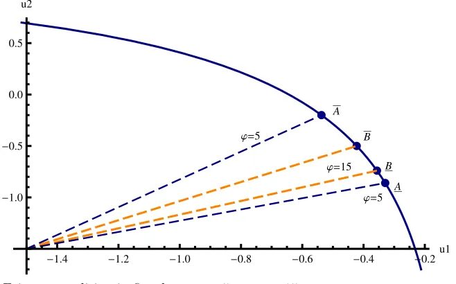
In Figure 1 we illustrate the fairness condition if there are only two types of households.13 _{One can see that the higherϕ, the smaller the set of utility allocations}

consistent with the fairness condition. Specifically, for ϕ = 5 all utility allocations on the segment (A, A) are consistent with the fairness condition. Withϕ = 15, only the smaller segment (B, B) is consistent with the fairness condition. As the strength of altruism approaches infinity, the left hand side of (13) approaches unity. That is,

∂ui(.)/∂xi = 1, for all i∈N. Under strict quasi concavity of the individual utility

functions, only a single utility allocation is consistent with the fairness condition. As the fairness condition requires equalization of marginal utilities, this singleton set need not correspond to an egalitarian utility allocation.

j=15 j=5

j=5

A

A B

B

-1.4 -1.2 -1.0 -0.8 -0.6 -0.4 -0.2u1 -1.0

-0.5 0.0 0.5 u2

Figure 1.Fairness condition in first-best;ϕ= 5 vs. ϕ= 15.

12

In fact, it can be shown that the existence of such a fairness condition is also implied by the presence of pure (instead of genuine) altruism in the utility function.

13

In the next step, we discuss the tax instruments required for the implementa-tion of the first-best allocaimplementa-tion characterized by equaimplementa-tions (11) – (13). That is, we analyze how the government has to set taxes such that households realize the efficient allocation as a solution to their maximization problem described above. There are two reasons why the government wants to impose taxes. First of all, it wants to redistribute resources since households differ in earning abilities. In ad-dition, redistribution is also implied by the presence of altruism which limits the set of allocations considered as fair. As a personalized lump-sum transfer/tax is available to the government, it can redistribute without distortions. Second, the government wants to correct for the externalities induced by the consumption of the status good. For the sake of simplicity we assume that no tax revenues have to be raised to finance public good expenditures, i.e. taxes are only used to redistribute resources and to internalize the consumption externalities.

When contrasting conditions (11) and (12) with conditions (4) and (5) describing the households’ optimality condition, one can see that in general a personalized commodity taxtz,i in addition to the personalized lump-sum element is required to

implement the first-best allocation as a competitive equilibrium.14 _{A personalized}

commodity tax is required if the externality is non-atmospheric, because in this case the Ψi differ between households. If the externality is atmospheric, a uniform tax

on status consumption in addition to the lump-sum element suffices to implement a first-best allocation. Commodityxstays untaxed in first best as the externality can be fully internalized withtz,i and redistribution can be achieved throughτi without

distortion. Proposition 1 summarizes this result.

Proposition 1 (First-best tax structure)

(i) If the externality is atmospheric, then optimal commodity tax rates are given by a single tax on z, t∗

z,i = Ψi = Ψ = t∗z and t∗x = 0, whether or not the consumption

externality is asymmetric.

(ii) If the externality is non-atmospheric, then optimal commodity tax rates are given by differentiated taxes on z, t∗

z,i = Ψi and t∗x = 0, whether or not the consumption

externality is asymmetric. (iii) The lump-sum elementτ∗

i is required for the efficient redistribution of resources.

14

Proof. See Appendix.

The intuition for this result is that if the externality is non-atmospheric the status consumption of some households is at the margin socially more harmful than the consumption of other households. This makes it desirable to tax the status con-sumption of different types at different rates. On the other hand, if the externality is atmospheric the consumption of all households is equally harmful at the margin and a uniform tax rate suffices.

3

Optimal second-best tax system

Personalized commodity taxes are required to implement a first-best allocation, but they are hardly a feasible policy instrument. Therefore, we now analyze the second-best optimal tax policy, when commodity taxes are restricted to be uniform across households. A Pareto efficient second-best tax system is a solution to the following problem:

max

tx,tz,τi,zi,i=1,...,n

v1(qx, qz, τ1, z1) + ϕ n

n

X

j=1

vj(qx, qz, τj, zj) (14)

subject to

vi(qx, qz, τi, zi) +

ϕ n

n

X

j=1

vj(qx, qz, τj, zj)≥vi i= 2, ..., n (µSBi ) (15)

tx n

X

i=1

xi+tz n

X

i=1 zi ≥

n

X

i=1

τi (λSB) (16)

zi =

1

n

n

X

j=1

aijzj i= 1, ..., n (γiSB) (17)

where again vi is some minimum utility requirement for household i. The index

SB for the Lagrange multipliers refers to second-best. We provide the first-order conditions for this problem in the Appendix.

3.1

Optimal commodity taxes

From the first-order conditions of this maximization problem the optimal commod-ity tax structure can be derived. To facilitate notation we define

ǫi ≡

1

n

n

X

j=1 γSB

j

It can be interpreted as the marginal social harm induced by the status consumption of householdimeasured in terms of the government’s tax revenues. We assume that

ǫi >0, i.e. that status consumption is socially harmful.15

In the Appendix we show that optimal commodity tax rates satisfy

sxx szx

sxz szz

tx

tz

=

₁

n

Pn

i=1ǫisizx

1

n

Pn i=1ǫisizz

, (19)

where compensated price effects are denoted bysi

zk =∂zicom/∂qkandsixk=∂xcomi /∂qk,

k = {z, x}, and the upper bar is used to denote the mean. By applying Cramer’s rule, (19) yields an implicit solution for the optimal second-best commodity taxes

t∗∗

z and t∗∗x .16

Proposition 2 (Second-best commodity tax structure: general case)

The optimal second-best commodity taxes are given by

t∗∗

z =

1

n(sxx

Pn

i=1ǫisizz −sxzPni=1ǫisizx)

szzsxx−szxsxz

, (20)

t∗∗

x =

1

n(szz

Pn

i=1ǫisizx−szxPn_i=1ǫisizz)

szzsxx−szxsxz

. (21)

The optimal tax on the status good is strictly positive. The sign oft∗∗

x is ambiguous.

Proof. See the Appendix. Observe that botht∗∗

z and t∗∗x are used to correct for the status externalities as they

both depend on the correction elementǫi.17 Thus, the ’additivity property’ derived

by Sandmo (1975) in a model with an atmospheric externality does not apply. The ’additivity property’ states that an externality is best addressed by imposing a tax directly on the externality-generating good and by leaving the rest of the tax sys-tem unaffected by the externality.18 _{In our framework it is optimal to also tax good}

15

In principleγSB

j and by thisǫi could also be negative. For a detailed discussion on the sign

of the Lagrange multiplier of constraint (17) see Eckerstorfer (2013). 16

The 2x2 sub-Slutsky matrix of the taxed goods is assumed to be non-singular and negative semi-definite, i.e. a solution to this system of equations exists and the determinant of this matrix is strictly positive.

17

The optimal tax formulas contain no redistributive component as personalized lump-sum taxes are available. If lump-sum taxes were restricted to be uniform,t∗∗

z andt∗∗x would also depend on

a redistributive term. This can be seen from the many-person Ramsey rule which we provide in the Appendix (equations (64) and (65)).

18

x to correct for the externality. The intuition for this result can be described in the following way. The government would want to tax the status consumption of different households at different rates. It wants to tax those households at a higher rate whose consumption is socially more harmful at the margin (see Proposition 1). But if commodity tax rates are restricted to be uniform across households such dif-ferential treatment of households is not possible. Therefore, the government wants to exploit other possibilities to channel the consumption decision of households in the desired direction, which can be achieved by changing the relative price structure through t∗∗

z and t∗∗x .19

Note that the presence of altruism has no impact on optimal commodity tax rates. This is because the incentive structure of households is not affected by this form of altruism. Households make their decisions independently of the parameter

ϕ as they consider average utility in the population as given. Thus, genuine altru-ism has no impact on the optimality conditions for an efficient allocation. It has, however, distributional consequences and gives rise to a fairness condition which we discuss in subsection 3.3.

To get a better understanding of the optimal commodity tax structure we now consider a number of special cases which provide some insights on how the opti-mal commodity taxes depend on the specific form of the reference level and on compensated price effects.

Corollary 1 (Second-best commodity tax structure: special cases)

(i) If the externality is atmospheric and symmetric the optimal commodity tax rates are given by

t∗∗

z =t∗z =ǫ, t∗∗x =t∗x = 0, (22)

with ǫ≡ǫi for all i.

(ii) If the externality is atmospheric and asymmetric optimal commodity tax rates are given by

t∗∗

z =t∗z =ǫ, t∗∗x =t∗x = 0, (23)

with ǫ≡ǫi for all i.

(iii) Ifsi

zx = 0orsizx=sizz for all i∈N and without any restriction on the reference

19

levels

t∗∗

z =

Pn i=1ǫisizz

Pn i=1sizz

, t∗∗

x = 0. (24)

(iv) Ifsi

zx= 0 or sizx=sizz for all i∈N and only household n is responsible for the

formation of the reference level, such that aij = 0 for j = 1, ...,(n−1) and aij =n

for j =n then

t∗∗

z =ǫn

sn zz

Pn i=1sizz

, t∗∗

x = 0. (25)

Optimal commodity taxes in Corollary 1 follow immediately from (20) and (21). Case (i) refers to a scenario where there is a unique reference level (for example the average consumption of the status good) while in case (ii) reference levels differ between households. From cases (i) and (ii) it can be seen that good x needs not to be taxed in the optimum if the externality is of the atmospheric type, no matter whether the externality is asymmetric or not. The optimal tax on the status good is equal to the marginal social harm of status consumption ǫ if the externality is atmospheric, again no matter whether the externality is asymmetric or not. Note, however, that the expressions forǫ differ between cases (i) and (ii) as ǫdepends on the different values for aij (see (18)). Thus, whether the externality is symmetric

or not has no impact on the optimal commodity tax structure but on the optimal level of t∗∗

z . Further, observe that if the externality is atmospheric a uniform tax

rate on the status good suffices to fully internalize the externality, and, together with the lump-sum element, a first-best allocation can be reached.

From cases (iii) and (iv) it can be observed that for the optimal commodity tax structure also the structure of compensated price effects is crucial. Given general reference levels, imposing a tax on the nonpositional good is not optimal if com-pensated cross price effects are zero or if the comcom-pensated cross price effects are equal to the own compensated price effect for the status good.20 _{Then households}

respond in such a way totx that no additional correction of the externality can be

attained. The structure of compensated price effects also has a strong impact on

t∗∗

z as can be seen from the reduced tax formulas in (24) and (25). Observe that in

cases (iii) and (iv) the externality is non-atmospheric and, thus, the marginal social harm of status consumption ǫi differs between households. This implies that the

20

Note that in this case sxx > szz which follows from the negative semi-definiteness of the

optimal tax rate on the status good is higher if those households whose consumption is socially more harmful at the margin also have a higher substitution effect due to a price increase of the status good. This can be seen in particular for case (iv) where only the consumption of householdnis responsible for the status externality.

3.2

Optimal lump-sum taxes

In this subsection we briefly discuss the optimal second-best lump-sum element. As personalized lump-sum taxes or -transfers are available, redistribution can be achieved in a non-distortionary way in this economy. In the optimum the social marginal utility of income is set equal to its marginal cost for all households. This follows immediately from the first-order condition for τi from problem (14) – (17)

which can be written as

θSB i

λSB

∂vi

∂τi

=M SCi, (26)

with θSB

i ≡ µSBi +ϕ/n

Pn

j=1µSBj and where the marginal social cost of income

(M SCi) is defined by

M SCi ≡1−tx

∂xi

∂τi −tz

∂zi

∂τi

+ǫi

∂zi

∂τi

. (27)

The first three terms on the right-hand side of (27) reflect the budget cost of a marginal income increase, and the last term denotes the social harm caused by that income increase due to an increase in status consumption. We now want to find out whether or not in a second-best tax system the lump-sum transfers are also used to correct for the externalities. In first-best, the externalities can be fully internalized by personalized commodity taxes. Then the lump-sum element is not needed for externality correcting purposes and serves only for the redistribution of income. However, in the second-best case the externalities can not be fully internalized due to the restriction that commodity taxes have to be uniform across households. Then one might suspect that also the lump-sum element is required to correct for the externalities. Plugging the optimal commodity taxes given by (20) and (21) into (26) reveals that, in general, a term depending on ǫi, and therefore on the

externality, remains. This implies that the optimal second-best lump-sum element

τ∗∗

i indeed depends onǫi.21 The intuition for this result is thatt∗∗z might overcorrect

21

This is not the case if the externality is atmospheric. Then the externalities can be fully internalized witht∗∗

z alone and a first-best allocation can be reached. In this caseM SCi is equal

for the status consumption of some households with low ǫi and undercorrect for

the status consumption of other households with high ǫi. The lump-sum element

can then be used to compensate those whose status consumption causes little social damage (lowǫi) and to extract income from those whose consumption is particularly

harmful (highǫi).

To illustrate this point, consider case (iv) of Corollary 1, where only the status consumption of household n causes an externality. In addition assume that there are no compensated cross price effects. By plugging the expressions for t∗∗

z and t∗∗x

from (25) into (26) one gets

θSB i

λSB

∂vi

∂τi

= 1− ∂zi

∂τi

(ǫn

sn zz

Pn i=1sizz

−ǫi)

| {z }

∆i

. (28)

Observe thatǫi = 0 for all i= 1, ..., n−1 and ǫn>0. Thus, ∆i is positive for these

households, while ∆n is negative as snzz/

Pn

i=1sizz < 1. This implies M SCi < 1

for i = 1, ..., n−1 und M SCn > 1. As marginal utility of income is decreasing in

income, the externality has a positive impact on the lump-sum element for those whose consumption does not cause an externality and a negative impact on the lump-sum element for householdn who is responsible for the externality. This is in accordance with the intuition provided above, that the lump-sum element is used to compensate those whose consumption is overcorrected by the commodity taxes and to extract income of those households whose consumption is undercorrected. Note that this argument only applies if the externality is non-atmospheric. If the externality is atmospheric it can be fully internalized withtzalone. Then ∆i = 0 for

alliand the government would setτiat its first-best level. Proposition 3 summarizes

this result.

Proposition 3 (Second-best lump-sum element)

(i) If the externality is non-atmospheric then in a second-best tax system also the lump-sum element τ∗∗

i serves to correct for the externality.

(ii) If the externality is atmospheric then τ∗∗

i = τi∗ as the externality can be fully

internalized through t∗∗

3.3

Fairness condition

We have shown that the presence of altruism has no impact on the optimal com-modity tax structure. However, similar to the first-best case, also in second-best a fairness condition exists which limits the set of allocations consistent with the Pareto criterion. There exists a set of allocations which would be Pareto efficient with purely egoistic preferences but which does not satisfy the Pareto criterion if households are altruistic. Intuitively, at such allocations altruistic households would prefer to give income away to those with very little income instead of consuming it on their own. Such a reallocation would make all households better off leading to a Pareto improvement.22 _{Since, in our framework there is no mechanism for}

households to give money directly to poorer ones, optimal tax policy is affected by the fairness-condition. In second-best, the fairness condition is given by:

1 +ϕ

ϕ ≥

1

n

n

X

j=1

∂vi/∂τi

M SCi

∂vj/∂τj

M SCj

(29)

for all i = 1, ..., n. From (29) it can be seen that in second best the average ratio of marginal utilities of income is weighted by M SCi. The fairness condition (29)

states that for an allocation to be Pareto efficient the average ratio of the marginal utility of income of household i to that of all other households must not be too large. Interestingly, in the second best case more inequality towards household i is tolerated if the marginal social cost of increasing the income of that household is large. From (27) it can be seen thatM SCi increases with the marginal social cost

of status consumption of householdi, as given byǫi. That is, if the status

consump-tion of household i is particularly harmful at the margin, then more inequality is tolerated with respect to that household.

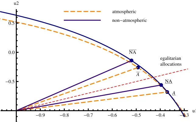
In Figure 2 we illustrate this point for two types of households. The figure shows the impact of a consumption externality being non-atmospheric rather than atmospheric on the set of utility allocations that are consistent with the fairness condition in second-best. A shift from an atmospheric to a non-atmospheric exter-nality goes along with a shift inM SCi, as in contrast to an atmospheric externality

22

a non-atmospheric externality implies thatǫi differs between households. The

yel-low dashed lines indicate the utility possibility frontier and fair allocations (segment betweenAandA) for the case of an atmospheric consumption externality. The solid blue lines show the respective utility allocations for the non-atmospheric consump-tion externality with aj1 > aj2, j = 1,2, i.e. the consumption of type 1 is socially

more harmful at the margin (ǫ1 > ǫ2).23

In order to gain intuitive understanding of this result (see Figure 2), we consider the effects of raising aj1 and lowering aj2 — initially starting ataj1 =aj2 = 1. The

slope of the utility possibility frontier is given by the right hand side of (29), with

i= 1. Graphically, the fairness condition, as given by (29), defines upper and lower bounds of the slope of the utility possibility frontier.

The slope of the Pareto frontier increases when raising aj1 and lowering aj2.

Intuitively, a given redistribution (dτ1 <0, dτ2 >0) increases ˜v2 by more in case of

the non-atmospheric consumption externality as opposed to the atmospheric one. In case of the non-atmospheric consumption externality, the redistribution moves away resources from the main externality generator. As a consequence, ¯zi is lowered

for all households.

As the slope of the Pareto frontier increases, the set of allocations satisfying the fairness condition shifts up and to the left, as depicted in Figure 2. The fairness condition imposes a requirement on the utility allocation that is very intuitive. As consumer 1 has become the main generator of a negative consumption externality, the fairness condition demands a redistribution of lump sum transfers away from consumer 1 towards consumer 2. In Figure 2, this requirement shows up as a shift of the segment of fair utility allocations towards northeast.

23

NA

NA

A

A

egalitarian allocations atmospheric

non-atmospheric

-0.9 -0.8 -0.7 -0.6 -0.5 -0.4 -0.3

u1

-0.5

0.0 0.5 u2

Figure 2. Fariness conditions in second-best: atmospheric vs. non-atmospheric externality;

ϕ= 5.

We obtain a similar result if there is a change in the degree in positionality

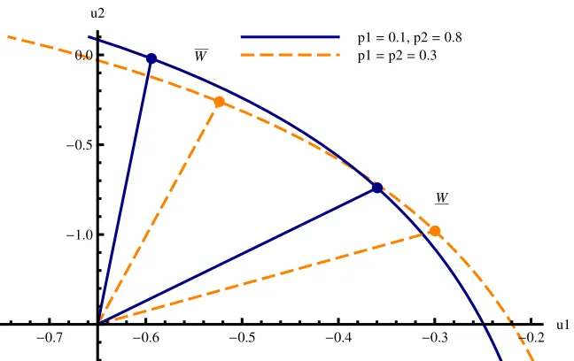
pi (for the functional specification, see Section 5). In Figure 3 we compare the

segments of fair utility allocations for two scenarios. In the first scenario indicated by the yellow dashed line both households have the same degree of positionality, while in the second scenario (solid blue line) household 2 is more positional than household 1. One observes that the segment shifts upwards implying that in the second scenario more inequality is tolerated with respect to household 1 and less with respect to the (now) more positional household 2. The key to understand this shift is that in scenario 2 for a marginal rise in lump sum transfers, household 2 gains more utility (from increased z consumption, and from shifting consumption fromxto z) than household 1 due to the higher importance of status consumption for household 2 as compared to household 1. As a consequence (the absolute value) of the slope of the Pareto frontier v1,τ1/v2,τ2 increases. That is, the investigated

changes inpi steepen the Pareto frontier, as can be seen in Figure 3. As the fairness

conditions in (29) put constraints on the (minimum- and maximum-) steepness of the Pareto frontier, the steepening of the Pareto frontier — due to changes inpi —

W

W

p1=0.1, p2=0.8

p1=p2=0.3

-0.7 -0.6 -0.5 -0.4 -0.3 -0.2

u1

-1.0 -0.5

0.0 u2

Figure 3.Fariness condition in second-best: variation in degree of positionalitypi; ϕ= 5.

4

Optimal taxes under a non-welfarist

govern-ment

Should the government accept status effects in its welfare criterion? Concerns for status and relative position are basically a form of jealousy and envy and one can question whether such behavior has to be respected by the policy maker. In this section we analyze the optimal tax policy of a government which knows that house-holds care about status effects but which does not want to include status preferences in the welfare criterion, i.e. the government’s and households’ preferences differ. So far, the literature has paid almost no attention to the idea that the presence of relative concerns in the social objective might have to be questioned. An exception is Kanbur et al. (2006) who discuss this issue in a survey article on non-welfarist optimal taxation.

additively. Preferences of households are described by the concave utility function

˜

ui(xi, zi, li) +mi(ri) +

ϕ n

n

X

j=1

(˜uj(xj, zj, lj) +mj(rj)), (30)

where ri ≡ zi/zi. We assumemr >0 and mrr ≤ 0 for alli = 1, ..., n. The optimal

decision of a household is, again, described by conditions (4) and (5) which can also be written as

∂u˜i/∂zi

∂u˜i/∂xi

+ 1

zi

∂mi/∂ri

∂u˜i/∂xi

| {z }

˜ Ψi

= 1 +tz 1 +tx

, (31)

∂u˜i/∂li

∂u˜i/∂xi

= wi 1 +tx

. (32)

We call ˜Ψi the part of theM RSzxi that stems from relative consumption concerns,

that is it tells how much of good x a household is willing to give up for the better relative position an additional unit of z provides. Note that in general ˜Ψi differs

between households.

The government knows that households base their decisions on the utility func-tion in (30) but it behaves in a paternalistic way and ignores mi(ri) in its welfare

criterion. Let the indirect utility function of a household be given by

˜

ui(zi∗(·), x∗i(·), l∗i(·))

| {z }

˜

vi(qx,qz,τi,zi)

+mi

z∗

i(·)

zi

| {z }

si(qx,qz,τi,zi)

+ϕ n n X j=1      ˜

uj(z∗j(·), x∗j(·), l∗j(·))

| {z }

˜

vj(qx,qz,τj,zj)

+mj

_z∗

j(·)

zj

| {z }

sj(qx,qz,τj,zj)

     . (33) The government considers only ˜vi +ϕ_nPnj=1v˜j in the welfare criterion. Hence, the

altruistic part of individual utility is included in the welfare criterion while the utility partsi emerging from the relative position of households will be omitted.24

4.1

Characterization of first-best allocations

We first characterize first-best allocations from the perspective of the government. Assume again that the government can directly determine xi, zi, li for each

house-holdi. Then an efficient first-best allocation from the perspective of the government

24

One implication of this is that the envelope theorem has to be used with care when taking derivatives of ˜vi. For example Roy’s identity becomes ∂

˜

vi

∂tz =−zi

∂˜_vi

∂τi −(

∂si

∂tz +zi

∂si

is a solution to the problem

max

xi,zi,li,i=1,...,n

˜

u1(x1, z1, l1) + ϕ n

n

X

j=1

˜

uj(xj, zj, lj) (34)

subject to

˜

ui(xi, zi, li) +

ϕ n

n

X

j=1

˜

uj(xj, zj, lj)≥ui i= 2, ..., n (˜µF Bi ) (35)

n

X

i=1 xi+

n

X

i=1 zi =

n

X

i=1

wi(1−li) (˜λF B) (36)

(37)

Observe that the government ignores the reference consumption levels and their impact on private utility in its maximization problem. In the Appendix, we pro-vide the first-order conditions for this problem from which the following optimality conditions can be derived:

∂u˜i/∂zi

∂u˜i/∂xi

= 1, (38)

∂u˜i/∂li

∂u˜i/∂xi

=wi, (39)

1 +ϕ

ϕ ≥

1

n

n

X

j=1

∂u˜i/∂xi

∂u˜j/∂xj

, (40)

for all i = 1, ..., n. From (38) and (39) it can be seen that if households had no relative consumption concerns, the government would not want to distort their con-sumption and leisure decision. But since households care about status concon-sumption, the government wants to distort the decision of households so that they behave as if they had no status concerns. In other words, the government wants to correct for the status preferences. In addition, similar to the welfarist case, the fairness condi-tion given by (40) limits the set of allocacondi-tions consistent with the Pareto criterion. This fairness condition also holds in the non-welfarist case because the government respects altruism to be part of the welfare criterion.25

In order to see which tax instruments are required to implement a first-best allo-cation, one has to contrast conditions (38) and (39) with the optimality conditions

25

of a household given by (31) and (32). Similar to the welfarist case, a personal-ized commodity tax ˜t∗

z,i = ˜Ψi on the status good, in addition to the personalized

lump-sum element, is required to implement a first-best allocation as a competitive equilibrium. Only if ˜Ψi is constant across households, a uniform commodity tax

on all households would suffice. In contrast to the welfarist case, whether or not a uniform tax on the status good suffices to implement the first-best allocation does not depend on whether the externality is atmospheric or not. A uniform tax rate on the status good suffices if the externality is symmetric — which implies that

zi = z — and if mr/u˜x is constant across households. A personalized commodity

tax is required in the non-welfarist case if different households are willing to give up different amounts of x for the better relative position an additional unit of z

provides. This is the case if ˜Ψi differs across households. Note that the nature of

the externality does not affect the first-best tax rate if ∂M RSzx/∂zi = 0, as then

the household decision does not depend onzi. Proposition 4 summarizes this result.

Proposition 4 (Non-welfarist government: first-best tax structure)

(i) In general optimal commodity tax rates are given by differentiated taxes on z, ˜

t∗

z,i = ˜Ψi andt˜∗x = 0, whether or not the consumption externality is non-atmospheric.

(ii) If the externality is atmospheric and symmetric and if mr/u˜x is the same for

all households, then optimal commodity tax rates are given by a single tax on z, ˜

t∗

z,i = ˜Ψi = ˜Ψ = ˜t∗z and ˜t∗x= 0.

(iii) The nature of the consumption externality has no impact on ˜t∗

z and ˜t∗x if

∂M RSzx/∂zi = 0.

(iv) The lump-sum elementτ˜∗

i is required for the efficient redistribution of resources.

Proof. See Appendix.

4.2

Optimal second-best tax system

If personalized commodity taxes are not feasible, a second-best tax system, from the perspective of the government, is a solution to the following problem:

max

tx,tz,τi,zi,i=1,...,n

˜

v1(qx, qz, τ1, z1) + ϕ n n X j=1 ˜

vj(qx, qz, τj, zj) (41)

subject to

˜

vi(qx, qz, τi, zi) +

ϕ n n X j=1 ˜

vj(qx, qz, τj, zj)≥vi i= 2, ..., n (˜µsBi ) (42)

tx n

X

i=1

xi+tz n

X

i=1 zi ≥

n

X

i=1

τi (˜λSB) (43)

zi =

1

n

n

X

j=1

aijzj i= 1, ..., n (˜γiSB) (44)

The first-order conditions for this problem are provided in the Appendix. Note that the only difference to problem (14) – (17) is the objective function in which the status part of the utility function is now omitted. Still, ˜vi is affected by the

reference level through the effect ofzi onx, z, l.26 Thus, when designing the optimal

tax system the effect of taxes on the reference levels has to be taken into account, even though the direct impact of zi on individual utility is not considered.

From the first-order conditions of problem (41) – (44) one can derive an implicit solution for the optimal second-best commodity taxes chosen by a non-welfarist government.

Proposition 5 (Non-welfarist government: second-best commodity taxes)

The optimal second-best commodity taxes from the perspective of a non-welfarist government are given by

˜

t∗∗

z =

1

n(sxx

Pn i=1 ˜ θSB i ˜ λSB 1 zi ∂m ∂ris

i

zz −sxz

Pn i=1 ˜ θSB i ˜ λSB 1 zi ∂m ∂ris

i zx)

szzsxx−szxsxz

+

1

n(sxx

Pn

i=1˜ǫisizz−sxzPn_i=1˜ǫisizx)

szzsxx−szxsxz

, (45)

26

The sign of ˜vz is ambiguous. In contrast to the previous section, now the government only

takes the indirect effect ofzion ˜ui(x, z, l) through its effect on demand forx, z, linto account and

˜

t∗∗

x =

1

n(szz

Pn i=1

˜

θSB i

˜

λSB

1

zi

∂m ∂ris

i

zx−szxPn_i=1

˜

θSB i

˜

λSB

1

zi

∂m ∂ris

i zz)

szzsxx−szxsxz

+

1

n(szz

Pn

i=1ǫ˜isizx−szxPn_i=1˜ǫisizz)

szzsxx−szxsxz

, (46)

where θ˜SB

i ≡µ˜SBi +ϕ/n

Pn

j=1µ˜SBj and ǫ˜i ≡n−1Pn_j=1(˜γjSB/˜λSB)aji.

Proof. See Appendix.

The optimal commodity tax rates depend on two terms now. The first term can be interpreted as the preference correcting part of the optimal tax formulas. From the perspective of the government households consume too much of the status good and it wants to deter individuals to purchase good z just for status reasons. Therefore, this term is strictly positive in the case of ˜t∗∗

z , making the status good more

expen-sive. Note that ˜t∗∗

x also depends on a preference correcting part, given by the first

term on the right-hand side (46). The reason is similar to the welfarist case in which

tx is used to correct for the status externality. Due to differences across households

in their willingness to pay for additional status the government would want to tax status consumption of each household at a different rate. Since it is restricted to use a single rate, it is optimal to use other tax instruments to correct for status preferences. The sign of the correction term in the case of ˜t∗∗

x is ambiguous.

The second term on the right hand side of (45) and (46) looks very similar to the term determining the optimal commodity tax rates in the welfarist case. However, its interpretation is different as ˜ǫi differs from ǫi. If the government has a welfarist

objective function,ǫi basically describes the marginal welfare cost of an increase in

the externality levelzi. In the case of a non-welfarist government there is no direct

welfare loss associated with an increase of zi. But since demand for x, z, l reacts

to changes in the reference levels there is an indirect effect of zi on the objective

function and on commodity tax revenues and these effects are summarized by ˜ǫi.

Thus, when determining ˜t∗∗

z and ˜t∗∗x the government has to take the effect of taxes

on the reference levels into account, even though it has no externality-correcting motive.

Corollary 2 (Non-welfarist government: second-best commodity tax struc-ture - special cases)

(i) If the externality is atmospheric and symmetric and if θ˜SBi

˜

λSB

∂mi

∂ri =

˜

θSB

˜

λSB

∂m

∂r for all

i∈N, optimal commodity tax rates are given by

˜

t∗∗

z = ˜t∗z =

˜ θSB ˜ λSB 1 z ∂m

∂r , ˜t

∗∗

x = ˜t∗x = 0. (47)

(ii) Ifsi

zx= 0 orsizx=sizz for alli∈N and without any restriction on the reference

levels ˜ t∗∗ z = 1 Pn

i=1sizz n X i=1 ˜ θSB i ˜ λSB 1 zi ∂m ∂ri

si_zz +

n

X

i=1

˜

ǫisizz

!

, ˜t∗∗

x = 0. (48)

Proof. See Appendix.

Case (i) refers to a scenario in which there is a unique reference level and in which the consumption of all households is weighted equally in the formation of that reference level. If in addition θ˜SBi

˜

λSB

∂mi

∂ri is the same for all households then the

first-best allocation can be implemented without personalized commodity taxes and good

xneeds not to be taxed. This statement is equivalent to the one in Proposition 4 (ii). Observe that for a welfarist government a uniform tax on the status good in addition to the lump-sum element suffices to implement the first-best allocation as soon as the externality is atmospheric (see Corollary 1). For a non-welfarist government more conditions are required. This is because a non-welfarist government has to take two aspects into account when correcting for status consumption, namely correction of preferences and correction of the indirect effect of the reference level on social welfare. For the former the heterogeneity in preferences among households for status consumption matters, for the latter the heterogeneity among households in the generation of the reference levels matters.

With respect to the optimal-lump sum element, a similar result to the one provided in the welfarist case can be derived. By plugging optimal commodity taxes into the first-order condition for ˜τi, it can be seen that ˜τi∗∗ also serves to

correct for status preference if a uniform tax on the status good does not suffice to fully correct for status preferences. Loosely speaking, the lump-sum element can be used to compensate those who have no or only a very weak taste for status and whose consumption of goodz is overcorrected by the commodity taxes. From those who have a very strong taste for status, additional correction of status consumption can be achieved by extracting income through the lump-sum element.

Also in second-best a non-welfarist government has to take a fairness condition into account which limits the set of allocations consistent with the Pareto crite-rion. The reason is that the government respects altruism to be part of the utility function. Formally the fairness condition is now given by

1 +ϕ

ϕ ≥

1

n

n

X

j=1

∂˜vi/∂τ˜i

^

M SCi

∂v˜j/∂τ˜j

^

M SCj

(49)

for alli= 1, ..., n.27 _{Thus, again for an allocation to be Pareto effcient the weighted}

average ratio of the marginal utility of income between household i and all other households must not be too large.

Interestingly, the structure of an optimal tax system of a welfarist government looks similar to that of a non-welfarist government. However, taxes are used for different reasons in the two scenarios. In the case of a welfarist government, the main objective is to correct for the status externalities, while a non-welfarist government wants to correct for the status preferences of individuals. In order to be able to make comparisons with respect to the magnitude of optimal commodity taxes in the two scenarios and to study the quantitative impact of the reference levels on optimal taxes we conduct some numerical simulations, which we present in the next section.

27

In the non-welfarist case we define the marginal social cost of increasing income for household

ibyM SC^i≡1−tx∂x_{∂τ i}i −tz∂z_∂τii + ˜ǫi

∂zi

∂τ i. For a derivation of (49), we proceed in the same way as

5

Results from Numerical Simulations

The above propositions imply the qualitative result that the nature of the con-sumption externality does have an impact on the first-best and second-best ef-ficient commodity tax rates both for a welfarist and for a non-welfarist welfare criterion. Considering reasonable calibrations, three main quantitative questions suggest themselves. First, for a given consumption externality (benchmark case), how different are first-best and second-best efficient commodity tax rates between the welfarist and the non-welfarist case? Second, what are the effects of the nature of the consumption externality – whether it is atmospheric or non-atmospheric, whether it is symmetric or asymmetric – on the first-best and second-best com-modity tax rate of the positional good both in the welfarist and the non-welfarist case? Third, in a second-best setting, what is the impact of the nature of the con-sumption externality on the commodity tax rate of the non-positional good, which is essentially zero in the first-best?

Numerical simulations, addressing these questions, are presented in the follow-ing. The results of those simulations arenot intended to suggest precise first-best or second-best tax rates on (non-)positional goods. Rather, they are intended to pro-vide a rough indication of how important the nature of the consumption externality for efficient tax rates – under a reasonable calibration – is. Therefore, the numer-ical simulations focus on the change of efficient tax rates due to the consumption externality rather than on thelevels of efficient tax rates.

We employ a simple specified model with two types of households, 1 and 2. There are n households. A share of η is of type 1, and a share of (1−η) is of type 2. Household types differ with respect to three attributes: preferences, labor productivity, and (possibly) externality coefficientsaij. Every household is endowed

with one unit of time. A household of type i receives a wage rate of wi per unit of

labor supplied. Preferences are represented by the following utility functions.

ui(xi, zi, li,z¯i) = αi lnxi+βi ln

zi

zi

¯

zi

pi

+γi lnli, i= 1,2, (50)

where ¯zi ≡ η ai1z1 +η ai2z2. Notice that these utility functions satisfy the

sepa-rability requirement of the non-welfarist case. Preference parameter pi represents

the strength of “positionality.” If pi = 0, the consumption reference level does not

household typei’s behavior. Johansson-Stenman et al. (2002) refer to [pi/(1 +pi)]

as the marginal degree of positionality.

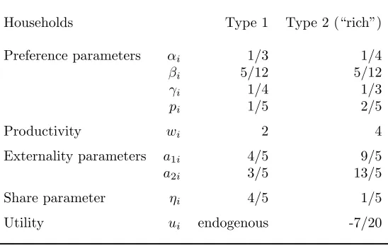
What we call baseline values of the background parameters is listed in Table 1. Unless stated otherwise, tables and graphs are based on these parameter values that imply standard stylized facts, as discussed below.

TABLE 1

Baseline values of background parameters

Households Type 1 Type 2 (“rich”)

Preference parameters αi 1/3 1/4

βi 5/12 5/12

γi 1/4 1/3

pi 1/5 2/5

Productivity wi 2 4

Externality parameters a1i 4/5 9/5

a2i 3/5 13/5

Share parameter ηi 4/5 1/5

Utility ui endogenous -7/20

Note.Notice thatη1a_i1+η2a_i2= 1.

With this parameterization, households of type 2 are considered significantly wealth-ier than households of type 1 (w2 > w1). Consistent with empirical evidence, those

households have a stronger impact on the consumption reference levels than type 1-households ( ai2 > ai1). Roughly, households of type 2 are rich and they are the

primary externality generators. These households are typically a small group within an economy. Therefore, we give this group just a small weight ((1−η) = 1/5).

Regarding the degree of positionality, we consider “rich” households as at least as positional as other households. Specifically, 2/5 = p2 > p1 = 1/5. Empirical

studies, including Alvarez-Cuadrado et al. (2012), Maurer et al. (2008), Ravina (2007), or Wendner and Goulder (2008) demonstrate that the marginal degree of positionality falls into the range [0.2,0.4]. Converting this range into a range for our pi yieldspi ∈ [0.25,0.67]. In our study we are quite conservative and consider

the low end of pi = 0.2, and the high end of pi = 0.4 (see Table 1).

Minimum utility of household type 2 is chosen to amount to a value of -0.35. As

parameterization, we fix the values of the other preference parameters (αi, βi, γi)

so that households choose an employment share in between (0.6,0.75), that is,

li ∈(0.25,0.4). Close to no empirical evidence exists for the coefficientsaij.

There-fore, most numerical simulations deal with the sensitivity of efficient tax rates with respect toaij. We are now ready to turn to our first question.

5.1

Welfarist versus non-welfarist tax rates

For the consumption externality as given by the baseline values (Table 1), how different are first-best and second-best efficient commodity tax rates between the welfarist and the non-welfarist case?

TABLE 2

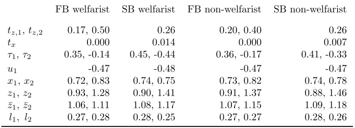
Welfarist versus Non-welfarist Tax Rates (baseline values)

FB welfarist SB welfarist FB non-welfarist SB non-welfarist

tz,1, t_z,2 0.17, 0.50 0.26 0.20, 0.40 0.26

tx 0.000 0.014 0.000 0.007

τ1, τ2 0.35, -0.14 0.45, -0.44 0.36, -0.17 0.41, -0.33

u1 -0.47 -0.48 -0.47 -0.47

x1, x2 0.72, 0.83 0.74, 0.75 0.73, 0.82 0.74, 0.78

z1, z2 0.93, 1.28 0.90, 1.41 0.91, 1.37 0.88, 1.46

¯

z1,z¯2 1.06, 1.11 1.08, 1.17 1.07, 1.15 1.09, 1.18

l1, l2 0.27, 0.28 0.28, 0.25 0.27, 0.27 0.28, 0.26

Note.FB = first-best, SB = second-best. In SB, a unique value fortz is given, astz1=tz2.

Table 2 suggests three main results. First, in the first-best, the efficient tax rate on the positional good is vastly sensitive with respect to a household’s strength of externality generation. For the baseline calibration, household type 2 is the primary generator of the consumption externality (ai2 > ai1,i= 1,2). In the welfarist

(non-welfarist) case,tz,2 is three times (twice) as large astz,1. Second, in the second-best,

the efficient tax on the non-positional good is different from zero, but quite small as compared to tz. In the welfarist (non-welfarist) case, tx = 1.4% ( tx = 0.7%).

welfare criterion — does not need to correct for thedirect effect of the consumption externality on welfare. In the first-best, therefore, the tax rates on the positional good tend to be lower and less different from each other than in the welfarist case. The less different thetz,i are in the first-best, the better a uniformtz in second-best

is able to mimic the first-best tax regime, thus, the lower is tx in the second-best.

As seen in Table 2, in the non-welfarist case the tax rate tx comes down to only

half the value it amounts to in the welfarist case.

5.2

Welfarist versus non-welfarist tax rates and the nature

of the consumption externality

This subsection considers the effects of the nature of the consumption externality on the first-best and second-best commodity tax rates of the positional good both in the welfarist and the non-welfarist case.

5.2.1 Efficient taxation in the first-best

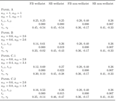
In Table 3 below, by systematically varying coefficientsaij, we identify the effects on

efficient commodity tax rates of the consumption externality being non-atmospheric rather than atmospheric as well as being asymmetric rather than symmetric. Specif-ically, Panel A considers an atmospheric and symmetric consumption externality (aij = 1). Panel B takes up a non-atmospheric and symmetric consumption

ex-ternality. Comparing Panels A and B allows some inference of the impact of the consumption externality being non-atmospheric rather than atmospheric on effi-cient taxation. Panels C.1 and C.2 investigate a non-atmospheric and asymmetric consumption externality. Comparing Panels B and C allows some assessment of the effects of the consumption externality being asymmetric rather than symmetric.

Table 3 offers several insights. Here we focus on the first-best tax regimes, for which tx = 0. In the following subsection, we focus on the second-best tax regimes.

In order to sharpen the differences between the welfarist and the non-welfarist case, preferences (50) are chosen such that only direct effects — effects via the welfare criterion — are caused by ¯zi.28

28

In other words, in the optimum, (xi, zi, li) are affected by pi but not by ¯zi. Thus, in the

non-welfarist case, individual behavior is independent of the composition of ¯zi. As the welfare

criterion is independent of ¯zitoo, the efficient non-welfarist tax regimes are identical across Panels

A to C.2. In contrast, in the welfarist case, the welfare criterion does depend on ¯zi. Thus, the