Non linear effects of the U S Monetary Policy in the Long Run

Munich Personal RePEc Archive

Non-linear effects of the U.S. Monetary

Policy in the Long Run

Olmos, Lorena and Sanso Frago, Marcos

Universidad de Zaragoza

2014

Online at

https://mpra.ub.uni-muenchen.de/57770/

Non-linear e¤ects of the U.S. Monetary Policy in

the Long Run

Lorena Olmos

University of Zaragoza

Marcos Sanso

University of Zaragoza

Abstract

We …nd non-linearities in the U.S. long-run relationships among trend in-‡ation, growth rate and …nancial frictions. Moreover, our results show that mismeasurements of the natural rate of interest deviate the trend in‡ation from its target, which is especially clear when monetary policy reacts preventively against in‡ation deviations. The long-run growth rate, the trend in‡ation and the natural rate of interest, speci…ed as time-varying, are jointly estimated over the period 1960:Q1-2013:Q2 by applying the Kalman …lter, following mainly Laubach and Williams (2003).

JEL code: C32; D52; E31; E52

Keywords: Kalman Filter, Trend In‡ation, Financial frictions, Growth

The authors acknowledge …nancial support from Ministerio de Ciencia e Innovación (Project ECO2009-13675) and Gobierno de Aragón (ADETRE research group).

1

Introduction

The existence of rigidities and frictions in the markets leads to non-neutral monetary

policies in the long run and non-linear e¤ects of some key variables according to

neokeynesian dynamic models with endogenous growth (Amano et al., 2009; Olmos

and Sanso, 2014a,b). These two features are especially clear when monetary policy

is conducted following some type of in‡ation targeting using the short-term interest

rate as the instrument or, in other words, following a Taylor rule (Taylor, 1993).

In this paper, we search for these nonlinearities for the case of the U.S. monetary

policy. In particular, we are interested in three non-linear e¤ects of the monetary

policy in the long run: the non-linear relationships between the trend in‡ation and

the growth rate, between the trend in‡ation and the external …nance premium and

between the growth rate and the error in the estimation of the natural rate of interest.

But the possibility of …nding this type of evidence is hindered by the problem of the

non-observable character of the long-term variables.

In fact, the relevance of the long-term variables is crucial for the performance

of the monetary policy carried out by central banks. Most speci…cations of Taylor

rules include one or more long-term variables, whose unobservability is an intrinsic

characteristic. The long-term variables which are usually incorporated into the

mon-etary policy rules are the natural interest rate, the in‡ation target and the potential

output1_{. As a result of the importance of these variables for the policy design, many}

1

contributions have been made on their estimation. Nevertheless, this task is not

straightforward.

There are several approaches to estimating unobservable variables. The simplest

techniques are the univariate …lters such as that of Hodrick-Prescott, but these

meth-ods are only based on the statistical properties of the series and ignore the connections

with other variables. Equilibrium models can also be built in order to estimate

unob-served series as is done in, among others, Neiss and Nelson (2003), Smets and Wouters

(2003), Giammaroli and Valla (2004) and Andrés, López-Salido and Nelson (2009),

but the resulting estimates are based on subjective assumptions and are prone to be

more volatile (Edge et al., 2008). As an alternative to the foregoing methods, and

admitting that this routine has been the object of some criticism2_{, our approach is}

based on the Kalman …lter applied to a semi-structural econometric model. This

pro-cedure has been implemented by many studies to estimate long-term values of several

economic variables. However, most of the papers that follow this technique do not

jointly estimate all the long-term variables involved in the monetary policy rules3

nor emphasize the long-term perspective. By contrast, our approach simultaneously

includes the natural rate of interest, the long-run growth rate and the steady-state

in‡ation in the estimation process in order to capture all the long-run interactions

we are interested in. 2

As discussed in Weber, Lemke and Worms (2008).

3

The …rst long-run variable we estimate is the natural rate of interest de…ned as

the long-run real rate of interest that ensures in‡ation stability and the reaching of

the potential output. The estimation of this variable has attracted the interest of

the literature since central banks conduct monetary policy through rules with this

rate as the intercept. Moreover, the gap between the natural rate of interest and

the actual real rate is very useful because it measures the monetary policy stance

and has predictive power for future in‡ation. Many empirical studies have tried

to assign a value to this rate, which initially was considered constant over time.

Afterwards, in a seminal paper, Laubach and Williams (2003) drop the assumption

of a …xed value4

and estimate the time-varying natural rate of interest (TVNRI)

for the U.S. by applying the Kalman …lter. The papers that have followed this

methodology are not few. Crespo-Cuaresma et al. (2004), Mésonnier and Renne

(2007) and Garnier and Wilhelmsen (2009) estimate the TVNRI for the euro zone,

Larsen and McKeown (2003) for the U.K., Manrique and Marques (2004) for the

U.S. and Germany, Basdevantet al. (2004) for New Zealand, Brzoza-Brzezina (2006)

for Poland and, recently, Bouis, et al. (2013) for Canada, the euro zone, Japan,

Sweden, Switzerland, the U.K. and the U.S. Combining Bayesian methods with the

Kalman …lter, Edge, Kiley and Laforte (2008) and Bjørnland, Leitemo and Maih

(2011) estimate the TVNRI for the U.S.5_.

4

They argue that this rate changes in response to shifts in preferences and in the trend growth rate of output. Trehan and Wu (2007) compare the implications of considering the natural rate of interest to be …xed or variable.

5

We also focus on the implications generated by the potential error that central

banks could commit in the estimation of the natural rate of interest. This issue has

been theoretically studied by, among others, Orphanides and Van Norden (2002),

Orphanides and Williams (2002), Tristani (2009) and Olmos and Sanso (2014b). We

approximate the gap between the correct and the estimated TVNRI and compute its

e¤ects on long-term in‡ation dynamics.

Estimating the TVNRI requires the estimation of the long-run trend of the

poten-tial output because, in the theoretical dimension, both variables are closely related.

In addition, this estimation is necessary because monetary policy rules are speci…ed

in terms of output deviations from the steady state level. Therefore, potential output

and, consequently, its growth rate, is the second unobservable variable we estimate.

But the TVNRI and the potential output are not the only variables involved

in the long run that are relevant for monetary policy. Trend in‡ation is another

long-term variable that plays an important role in its design and in its outcomes6

.

Like the potential output, it serves as a reference in the deviation measure of the

in‡ation rate as long as it coincides with the in‡ation target of the monetary policy

rule. Moreover, as it is pointed out in Olmos and Sanso (2014b), the potential

incorrect estimation of the TVNRI generates a gap between the in‡ation target and

its steady-state value that sets o¤ distortions in the long-run equilibrium. Therefore,

by including this variable in the estimation process, an increase in the robustness of

the analysis is expected as well as an expansion of the range of conclusions. In this

6_{In this regard, Ascari (2004) and Cogley and Sbordone (2008), among others, analyze the}

line, Leigh (2008) estimates the TVNRI for the U.S. through the Kalman …lter, but

all other unknown variables are overlooked. Moreover, a relevant topic we want to

study is the relationship between the long-run growth rate and the trend in‡ation.

Previous theoretical literature, such as Amano et al. (2009) and Olmos and Sanso

(2014a), shows the existence of a non-linear relationship between these two long-term

variables. And, despite the fact that the Kalman …lter provides a linear estimation,

we use the outcomes of the model to check the kind of connection between them

through a quadratic and a quantile regression.

Another issue we want to discuss is the role of …nancial frictions in the

determi-nation of the long-term main variables. Olmos and Sanso (2014a) show a connection

between …nancial frictions, the growth rate and the trend in‡ation in the long run

with some non-linear relationships. Ö¼günç and Batmaz (2011) follow the Laubach and

Williams (2003) procedure and include the risk premia for Turkey. They conclude

that the long-run evolution of this spread determines the natural rate of interest.

This link between …nancial frictions and the TVNRI is also studied empirically in

Archibald and Hunter (2001) for the New Zealand case.

Our database comprises time series for the U.S. during the period

1960:Q1-2013:Q2. The evolution of the estimates of the TVNRI, the long-run growth rate

of the economy and the steady-state in‡ation rate are in line with foregoing results.

Our estimates prove the negative e¤ect that …nancial frictions would cause on the

long-run growth rate, that potential misunderstandings of the TVNRI would deviate

long-run growth rate and the trend in‡ation is described as a nearly hump-shaped

curve.

The remainder of the paper is organized as follows. The second section describes

the methodology applied. In the third section, we present the estimation results,

carry out a quadratic and a quantile analysis of the relationships among the

long-run growth rate, the trend in‡ation and …nancial frictions, and study the e¤ects of

misunderstandings of the natural rate of interest. Finally, Section 4 summarizes the

main conclusions. The Kalman …lter procedure is detailed in the …rst appendix and

the state-space form of the model is explained in the second.

2

Estimation methodology for the unobservable

variables

To achieve the objectives stated in the previous section about the estimation of the

long-run unobservable variables, we extend the Laubach and Williams (2003)

semi-structural model by making some modi…cations. The core of the procedure, a

state-space model devoted to implementing the Kalman …lter, remains unchanged.

How-ever, we include a new state variable, the trend in‡ation. This extension complicates

the model but adds robustness to the whole estimation since it jointly estimates all

relevant variables in the long-term horizon. We also introduce some changes into the

model speci…cation in order to improve the consistency of the long-run implications

This empirical model is a small-scale simpli…cation of the New Keynesian

macro-economic model developed in Olmos and Sanso (2014a,b), where the main …ndings

we want to evaluate are the relationships among the long-run economic growth rate,

the trend in‡ation and …nancial frictions, as well as other relevant conclusions like the

e¤ects of potential errors in the estimation of the natural rate of interest. The

connec-tions established among these variables show the non-linear e¤ects of the monetary

policy in the long run.

The …rst equation of the model corresponds to the Phillips curve and describes

the evolution of the in‡ation rate ( t), an observable value. We de…ne the in‡ation

rate as the core consumer price index, which includes all items except food and

energy, and take the data from the Bureau of Labor Statistics. The quarterly series

is obtained as the monthly average value and then is seasonally adjusted with the

Tramo/Seats methodology. Once we have computed the quarterly in‡ation rate, the

data is annualized. We consider the in‡ation rate as a function of its own lags, the

output gap (zt), the trend in‡ation ( t) and a serially uncorrelated error term "t. In

this way, we ensure the consistency of the model in the long term because in‡ation

rate would equal its steady-state value, the trend in‡ation. The resulting equation is

the following:

t+1 = (L) t+ zzt+ (1 (L)) t+"t+1 (1)

where (L) is a lag-polynomial and z

is interpreted as the slope of the Phillips

The next relationship is a state equation equivalent to the reduced form of the IS

curve that explains the output gap, the percentage deviation of the real output from

its potential level. This variable depends on its own lags and on the measurement

error of the natural rate of interest, de…ned as the di¤erence between the ex-ante

real interest rate (Rt) and the natural rate of interest (Rnt). In turn, real interest

rate is gauged by subtracting the in‡ation expectations (Et t+1) from the short-term

nominal interest rate Rst

t , which is obtained from the Federal Reserve System

data-base. In‡ation expectations are computed by an 8-quarters forward-moving average

and nominal interest rate is equivalent to the federal funds e¤ective rate. Again, a

serially uncorrelated error term "z

t is included. This relationship is also consistent

with the long run because, in the absence of shocks and mismeasurement problems,

the output gap would be zero in the steady state:

zt+1 = z(L)zt+ r(Rt Rnt) +" z

t+1 (2)

where z_{(L) is a lag-polynomial. We assume, following Mésonnier and Renne}

(2007), a de…nition of the natural interest rate based on standard optimal growth

models. However, the speci…cation is slightly di¤erent and follows Bouiset al. (2013),

where the natural rate of interest is related to the long-run growth rate (gt) corrected

by a parameter7

@ and augmented by , the inverse of the intertemporal elasticity

of substitution in consumption, also interpreted as the relative risk aversion. An

intercept %is also included, which represents the time preference of consumers:

7

In terms of the Ramsey model, parameter @_{could be interpreted as a measure of the e¤ects of}

Rn_t =%+ (gt @) (3)

The long-run growth rate, equivalent to the growth of the potential output yt, is

explained as a function of its …rst lag, …nancial frictions (ft) and the trend in‡ation.

Financial frictions are proxied by the spread between the average majority prime

rate charged by banks on short-term loans to business and the 3-month Treasury bill

rate, both series collected from the Federal Reserve System database. This external

…nance premium is a standard simple measure of the frictions present in the …nancial

markets. An intercept and a serially uncorrelated error term are also included. In

the steady state, the growth rate would depend on a …xed value @ and also on the

trend in‡ation, as is theoretically shown in Olmos and Sanso (2014a):

gt=@(1 g) + ggt 1+ ft+{ _{t 1}+"g

t (4)

As can be seen, one main di¤erence between our speci…cation and those of Laubach

and Williams (2003) and Mésonnier and Renne (2007) is that growth of the potential

output is de…ned as a function of state and observed variables instead of a simple

AR(1) process. Moreover, our hypothesis regarding the order of integration of both

Rn

t and gt follows the approach of Mésonnier and Renne (2007) assuming highly

persistent but stationary variables driven by unobservable processes which capture

common low-frequency variations inRn

t and gt as well as idiosincratic ‡uctuations of

gt.

noted in equation (1), trend in‡ation would equal the in‡ation rate in the long run:

t+1 = t+ 1 Et t+1+"_t+1 (5)

Finally, the last equation is the identity that de…nes the output gap as the

dif-ference between the output (yt), built as the log of the real chain-weighted GDP in

billions of chained 2009 dollars taken from the Bureau of Economic Analysis, and the

log of its potential level:

zt=yt yt (6)

Summing up, the unobservable variables that we jointly estimate are(yt; gt; Rnt; t),

whilst the observed variables are( t; Rtst; yt; ft). We should note that shocks "t; "zt; " g t; "t

are independently and normally distributed and their variances are 2

; 2

z;

2

g;

2

,

respectively.

Having introduced the equations of the semi-structural model, we have to

artic-ulate the state-space model. Appendix A1 is devoted to presenting the state-space

representation which consists of the measurement equation and the transition

equa-tion. Afterwards, we are able to implement the Kalman algorithm (Kalman, 1960).

The basic intuition behind this procedure follows two steps. In the …rst, the system

makes a prediction based on the information available at a speci…c point of time. In

the next period, the …lter corrects this prediction by uploading the new information.

The maximum likelihood method is used to estimate the conditionally unbiased and

Kalman …lter mechanism8_.

3

Results for the U.S. economy

We now estimate the model speci…ed in the previous section. The quarterly data set

we have used refers to the United States in 1960:Q1-2013:Q2. It should be noted that

the Kalman …lter is very sensitive to the initial conditions. The technique we have

implemented to overcome this issue consists of several steps. Firstly, we carry out

a univariate estimation of each unobserved variable. To that end, we have applied

the Hodrick-Prescott …lter to the in‡ation rate, the real GDP and its growth rate

in order to obtain preliminary estimates of the trend in‡ation, the potential output

and the long-run growth rate, respectively. Secondly, we have estimated each

equa-tion including the series provided by the HP …lter with the purpose of assigning the

initial values to the parameters. This …rst estimation of the Kalman …lter generates

variances biased towards zero9

and, therefore, unsatisfactory results outside the

ac-ceptable values for the unobservable variables. Thus, we have to use the common

method of restricting some coe¢cients by calibrating the following parameters:

Following Bouis et al. (2013), one of the best candidates to gauge % is the

average of the actual real interest rate because it measures the trend value of

the natural rate of interest approximately. This approach is also used to set the

value of the intercept of the long-run growth rate equation@, equating it to the

8

Good references to understand this procedure are Harvey (1989) and Hamilton (1994).

9

sample average of the real output growth rates.

Due to the lack of consensus about the value of the parameter , we choose the

value 4.167, used in our theoretical model of reference, i.e. Olmos and Sanso

(2014a).

Finally, we calibrate 2

so that trend in‡ation accounts for 50% of the in‡ation

rate ‡uctuations.

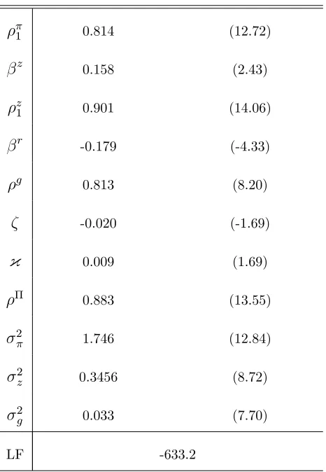
Table 1: Coe¢cient estimates

1 0.814 (12.72)

z

0.158 (2.43)

z

1 0.901 (14.06)

r

-0.179 (-4.33)

g _{0.813 (8.20)}

-0.020 (-1.69)

{ 0.009 (1.69)

0.883 (13.55)

2

1.746 (12.84)

2

z 0.3456 (8.72)

2

g 0.033 (7.70)

LF -633.2

z-Statistic in parenthesis. LF: Likelihood function.

We now explore the results of the model by analyzing the estimated coe¢cients

statistically signi…cant. Regarding the lags included for the in‡ation rate in (1), we

impose order 1 for the (L) lag-polynomial, whose coe¢cient is 1. Otherwise, the

coe¢cient associated with tin (1) loses weight and, consequently, the state estimates

become distorted. The signi…cativity criterion reveals that the lag-polynomial of the

output gap in (2) is of order 1. Both the slope of the Phillips curve z _{and the}

coe¢cient r_{, which drives the output gap in accordance with ‡uctuations in the}

di¤erence between the actual interest rate and its natural level, are higher than those

estimated by Laubach and Williams (2003) and Bouis et al. (2013)10

, but remain

within reasonable values. Financial frictions negatively a¤ect the long-run growth

rate, which can be seen from the negative value of . Trend in‡ation exerts the

opposite e¤ect because coe¢cient { has a positive sign, though the size is very low.

As the statistical signi…cance of these two linear e¤ects is at the limit of 10%, we go

deeper into this issue in the last part of the paper when we pose the question of the

non-linear e¤ects.

The estimation of the model with the features described above yields the evolution

of the unobserved variables displayed in Figure 1. We should clarify that these series

are two-sided estimates or smoothed estimates, that is, to compute them, the Kalman

algorithm has used the information of the full sample. In addition, we have discarded

the …rst few quarters because the estimates are outside the admissible range.

11

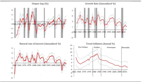
Figure 1: Estimates of the unobserved variables

Grey bars refer to the o¢cial recession dates provided by the National Bureau of Economic Research. Dashed lines represents the 90% con…dence interval.

Table 2 displays the statistical properties of the unobserved variables. Output gap

shows an expected path in the range (-6%,5%) with eight slowdowns corresponding to

the o¢cial recession dates of the U.S. economy11

, which also can be appreciated in the

long-run growth rate trajectory. This …rst inference seems to verify the accuracy of

the estimates. The sharpest declines of the output gap are situated at the beginning

of the sample and in the early 1980s recession, whilst the long-run growth rate reaches

its minimum value in 2008 during the …nancial crisis. The trajectory of the natural

11

rate of interest is obviously analogous to the long-run growth rate evolution because

the former is de…ned as a linear combination of the latter. Values of the long-run

growth rate and the natural rate of interest in 2008:Q4 seem to be atypical since

the troughs of both series are anomalously low for long-term references. Finally, the

trend in‡ation rises sharply from the late sixties to 1980, during the Pre-Volcker

era. After reaching its peak in the middle of Volcker’s presidency of the Federal

Reserve System, the trend in‡ation has constantly decreased leading to the so-called

Volcker disin‡ation. From the late-nineties, under the leadership of Greenspan, the

trend in‡ation has stabilized around a value of approximately 2%, level at which it

is assumed that FED locates its in‡ation rate target for the medium and long term.

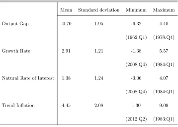
Table 2: Statistical properties of the estimated series

Mean Standard deviation Minimum Maximum Output Gap -0.70 1.95 -6.32 4.40

(1962:Q1) (1978:Q4) Growth Rate 2.91 1.21 -1.38 5.57

(2008:Q4) (1984:Q1) Natural Rate of Interest 1.38 1.24 -3.06 4.07

(2008:Q4) (1984:Q1) Trend In‡ation 4.45 2.08 1.30 9.09

3.1

Searching for nonlinearities

We have seen, in Table 1, that the estimation of the coe¢cient { is near zero and

that its corresponding p-value is slightly lower than 10%, so the linear relationship

between the long-run growth rate and the trend in‡ation is very weak. The same

remark can be made about the relationship between the external …nance premium

and the growth rate. These are not two counterintuitive results in the light of the

…ndings of Olmos and Sanso (2014a), because these outcomes may not mean the

absence of a relationship between the trend in‡ation and the long-run growth rate

and between the latter and the external …nance premium, but perhaps the model

speci…cation used is veiling relevant bivariate movements. The theoretical results we

have proposed to test in this paper are the presence of nonlinearities between these

two pairs of variables but, unfortunately, in the model to which the Kalman …lter

is applied, non-linear speci…cations can not be included. Although the Extended

Kalman …lter can integrate such speci…cations, its operation is very complex, so we

have opted for a two-step analysis. The …rst, already done, is to obtain estimates

of the state variables. In the second, we use these estimates of the unobservable

long-run variables to test the hypothesis established in Olmos and Sanso (2014a), a

hump-shaped relationship between the long-run growth rate and the trend in‡ation,

on the one hand, and a U-shaped relationship between the trend in‡ation and the

external …nance premium, on the other.

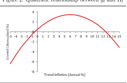
A simple way to look for non-linear relationships is to de…ne a quadratic equation.

^

gt= 0:52 + 0:98 ^t 0:08 ^2t + u^ g t

(1.42) (5.88) (-4.84)

(7)

where ^t and g^t are the trend in‡ation and the long-run growth rate series

esti-mated by the Kalman …lter,u^g_t refers to the residuals and the t-ratios are presented

in parentheses. In line with the foregoing theoretical results, the coe¢cient values

show a hump-shaped relationship between ^gt and ^t plotted in Figure 2. This very

signi…cant non-linear relationship indicates that, for low levels of trend in‡ation, the

long-run growth rate increases until ^t = 6% and, after this value, the growth rate

decreases with the trend in‡ation, reaching zero when it is 12.7% and -0.5%. The

an-nualized maximum potential growth is near 4%. But this outcome varies depending

on the sample considered. If we contemplate a period of in‡ation stability, such as

the subsample beginning in 1994 during which the Federal Reserve has reacted

pre-emptively against deviations of in‡ation from its target, the level of trend in‡ation

for which estimated growth is maximized drops markedly to ^t= 4%.

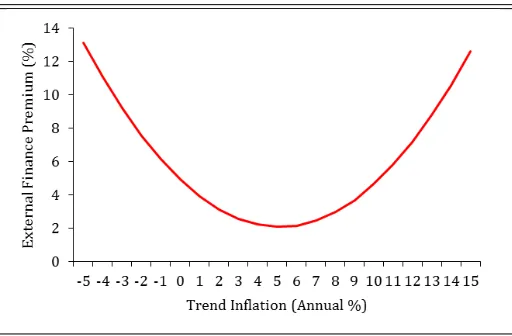
As in our previous exercise, we again perform this analysis to test for the link

between …nancial frictions and the trend in‡ation in the long run. Olmos and Sanso

(2014a) conclude that this connection has a U shape. Equation (8) presents the

estimated coe¢cients, where it can be seen that the U-shaped relationship found in

that paper, displayed in Figure 3, is corroborated. It should be noted that the level of

trend in‡ation for which estimated growth is maximized nearly matches the minimum

value of …nancial frictions.

ft= 4:90 1:11 ^t + 0:11 ^2t + u^ f t

(16.04) (-7.96) (7.69)

(8)

where u^ft are the residuals.

Figure 3: Quadratic relationship betweenft and ^t

Another way of searching for the nonlinearties we are interested in is to take into

account that the state estimates have been obtained using a speci…c linear model.

in‡ation and …nancial frictions with the long-term growth rate, looking for possible

nonlinearities. In doing so, we again try to verify if the theoretical results obtained in

Olmos and Sanso (2014a) are validated. We take the sample 1962:Q1-2013:Q2 in order

to avoid the initial distorted observations of the state estimates. The methodology

we adopt is based on a quantile regression but, in contrast to the common practice of

ordering observations according to the endogenous variable, we arrange the quantiles

according to an exogenous variable, the trend in‡ation. Thus, the speci…cation of our

equation of interest, which relates the long-term growth rate, …nancial frictions and

the trend in‡ation, is the same12

as (4), although levels of the explanatory variable

^_{t are distinguished. We opt for six quantiles because this is the largest number that}

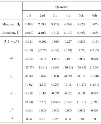
provides an acceptable number of observations in each quantile. Table 3 shows the

lower and the upper limit of each quantile, the estimated coe¢cients, the variance

and the coe¢cient of determination.

We expect a positive sign of { in the lower quantiles and a negative one in the

higher, what would resemble the inverted parabola obtained previously. For all the

quantiles except the last one and, consequently, for most of the sample, the

relation-ship can be described as an inverted U curve. However, when trend in‡ation is above

6.67% (last quantile), which occurs between 1973 and 1984, the estimated coe¢cient

is positive. Nevertheless, this scenario could be considered as an anomalous pattern

since, during those years, the two economic recoveries after strong downturns were

attached to a monetary policy that did not react severely to in‡ation deviations.

12_{We no longer include the trend in‡ation as a lag because that was a speci…c constraint of the}

Table 3: Quantile regression

Quantiles

1st 2nd 3rd 4th 5th 6th Minimum ^t 1.30% 2.09% 3.42% 4.35% 5.22% 6.67%

Maximum ^t 2.06% 3.40% 4.31% 5.21% 6.52% 9.09% @(1 g_{) 0.324 -0.262 0.085 0.227 0.263 -0.454}

(1.68) (-2.77) (0.26) (1.10) (1.74) (-2.22)

g _{0.973 0.804 1.054 0.947 0.905 0.921}

(25.77) (14.91) (9.86) (10.34) (20.83) (15.06) -0.161 0.026 0.006 -0.024 -0.014 -0.046 (-4.02) (2.60) (0.70) (-1.11) (-1.27) (-3.31)

{ 0.120 0.118 -0.035 -0.026 -0.031 0.085

(2.23) (2.82) (-0.56) (-0.52) (-1.21) (3.21)

2

0.004 0.002 0.003 0.005 0.003 0.009 R2

0.96 0.97 0.92 0.88 0.94 0.90 t-ratios are reported in parentheses.

With respect to the relationship between …nancial frictions and the long-run

growth rate, coe¢cient is statistically signi…cant at 5% only for the extreme lower

and higher values of the trend in‡ation, so the in‡uence is coherent with the

U-shaped relationship between the trend in‡ation and the external …nance premium.

For medium in‡ation rate levels, when the external …nance premium does not reach

not a¤ect, or positively a¤ect, the long-term growth rate. However, when the degree

of …nancial frictions increases, long-run growth could be negatively a¤ected by such

rigidities.

3.2

Long-run e¤ects of natural rate of interest

mismeasure-ments

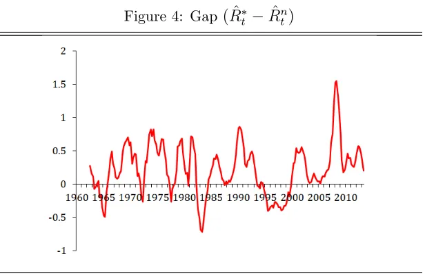
In order to capture other non-neutral and non-linear e¤ects of the monetary policy

in the long run, we approximate the real-time gap between the estimated and the

correct value of the natural rate of interest as the di¤erence between the one-sided

(R^t, …ltered) and the two-sided (R^nt, smoothing) estimates following Mésonnier and

Renne (2007). This is a proxy of the mismeasurement gap since the former estimation

takes into account the information available at the time of the estimation, as central

banks do, and the latter uses the full sample information of the signal variables, which

approaches the true value. In Figure 4, the evolution of the mismeasurement gap is

displayed.

This gap reaches a substantial size and, even if we do not consider the highest

deviations, the gap moves around values of( 0:5%;1%). When the mismeasurement

gap takes positive values, monetary policy tends to be more contractionary since the

intercept of the rule is higher than the endogenous value. Analogously, when the gap

is negative, monetary policy is more expansive. The average of the gap is near 0.25%

meaning that, on average, Federal Reserve implements a restrictive monetary policy

Figure 4: Gap( ^Rt R^nt)

Plot of the 2-quarter central moving average of the gap between the …ltered (R^_t) and the smoothing (R^n

t) estimation of the TVNRI

We now explore the potential implications of the existence of this gap from the

long-run perspective. This exercise is based on the theoretical work developed in

Ol-mos and Sanso (2014b), where it is concluded that central banks’ misunderstandings

in the estimation of the natural rate of interest a¤ect the long-run equilibrium by

deviating the steady-state in‡ation rate from its target. When the natural rate of

interest estimated by the central bank is higher than the correct value, trend in‡ation

is below its target and vice versa. Accordingly, the relationship between the deviation

of the natural rate and the gap of the trend in‡ation is negative.

Firstly, in order to carry out this analysis, we have to transform the trend in‡ation

series to be comparable with the mismeasurement gap. Hence, we have to calculate

the deviations of the trend in‡ation from the estimated target, the latter proxied as

its statistical mean. However, the evolution of the estimated trend in‡ation exhibits a

of this variable by way of the Bai-Perron methodology, which allows for the presence of

structural changes (see Bai and Perron, 1998, 2003) throughout the sample

1962:Q1-2013:Q2. The application of this methodology leads us to observe the existence of 5

di¤erentiated periods in the evolution of the trend in‡ation with the following break

points: 1970:Q3, 1979:Q2, 1986:Q4 and 1995:Q2. The estimated annualized values for

the mean of the trend in‡ation in the …ve subperiods are 4.1%, 6.1%, 7.5%, 4.9% and

2.3%, respectively. Secondly, with these averages, we can compute the deviations of

the trend in‡ation from the estimated target and relate them to the mismeasurement

gap. In order to smooth both series, characterized by strong ‡uctuations, we construct

the 2-quarter central moving averages for the trend in‡ation and the mismeasurement

gap.

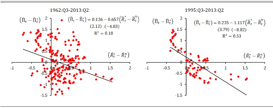
Figure 5: Trend in‡ation deviations from its target and mismeasurement gap

Scatter plot between the 2-quarter central moving average of (^t ^t) and (R^t R^ n t).

t-ratios in parentheses

^_{t is the estimated trend in‡ation and} ^

t is the estimated target, and the

mismea-surement gap R^_t R^n

t , whereR^t is the estimated intercept of the Taylor rule and

^

Rn

t is the estimated natural rate of interest.

This analysis reveals that the relationship is negative for the full sample as the

theoretical analysis predicts. However, if we divide the total sample into the speci…ed

periods detailed above, the results are not homogeneous. In the …nal period, which

is the largest one of the time intervals considered, the negative relationship is much

clearer than in the whole sample. These results lead us to think that, when

mone-tary policy was conducted through monemone-tary aggregates and the implicit or explicit

estimation of the natural rate of interest was not required, or monetary authorities

do not react against in‡ation deviations tightly enough, the mismeasurement gap

was not so relevant and was not so clearly transferred to the long-term in‡ation. So,

we can conclude that, with policies derived from Taylor rules whose priority is the

in‡ation stability, the natural rate of interest and its measurement become essential

for the monetary policy because measurement errors could in‡uence the long-term

equilibrium. These preliminary results seem to support this intuition and, therefore,

verify the negative relationship between the two gaps specially for the period in which

the Federal Reserve conducts monetary policy through in‡ation targeting rules which

4

Conclusions

In this paper, we analyze the long-run interactions of the U.S. unobservable

vari-ables included in the Taylor rules. Firstly, we look for the existence of nonlinearities

between the long-run growth rate, the trend in‡ation and …nancial frictions in the

long run. Through quadratic equations, we con…rm the existence of a hump-shaped

connection between the long-run growth rate and the trend in‡ation and a U-shaped

relationship between the latter and …nancial frictions. Then, by estimating a

quan-tile regression which distinguishes among levels of trend in‡ation, we corroborate

that hump-shaped connection if the trend in‡ation does not exceeds an upper

thresh-old. Moreover, especially for low and high levels of trend in‡ation, …nancial frictions

negatively a¤ect the long-run growth rate.

Furthermore, we approximate the gap between the real-time estimate and the

correct value of the natural rate of interest and study its e¤ects on the trend in‡ation

deviations from the target level. We prove that, for the whole sample, there is a

neg-ative relationship between the error in the estimation of the natural rate of interest

and the gap of the actual trend in‡ation and its target, as is concluded in the

theo-retical models developed in Olmos and Sanso (2014a,b). This negative relationship is

especially clear and signi…cant when monetary policy reacts aggressively against

in-‡ation deviations. In turn, deviations of the trend inin-‡ation from its target could also

a¤ect …nancial frictions and the long-run growth rate, since have been demonstrated

the interactions among these three key variables.

interest, the potential output and the trend in‡ation using U.S. data for the

1960:Q1-2013:Q2 period. Our procedure extends the methodology of Laubach and Williams

(2003), who implement the Kalman …lter to a semi-structural econometric model in

order to obtain the unobservable series, by including the trend in‡ation as a state

variable and …nancial frictions as an exogenous factor. The state estimates show

that the long-run growth rate and the natural rate of interest have experienced an

unprecedented decline during the …nancial crisis triggered in 2007, a pattern that is

not observed for the output gap. Meanwhile, the trend in‡ation has stabilized since

References

[1] Amano, R.; Moran, K; Murchison, S. and Rennison, A. (2009): "Trend

in‡a-tion, wage and price rigidities, and productivity growth," Journal of Monetary

Economics 56(3), pp. 353-364.

[2] Andrés, J.; López-Salido, D. and Nelson, E. (2009): "Money and the natural

rate of interest: Structural estimates for the United States and the euro area,"

Journal of Economic Dynamics and Control 33(3), pp. 758-776.

[3] Archibald, J. and Hunter, L. (2001): "What is the neutral real interest rate, and

how can we use it?,"Reserve Bank of New Zealand Bulletin 64(3), pp. 15-28.

[4] Bai, J. and Perron, P. (1998): "Estimating and testing linear models with

mul-tiple structural changes," Econometrica 66, pp. 47-78.

[5] Bai, J. and Perron, P. (2003): "Computation and analysis of multiple structural

change models," Journal of Applied Econometrics 18(1), pp. 1-22.

[6] Benati, L. and Vitale, G. (2007): "Joint estimation of the natural rate of interest,

the natural rate of unemployment, expected in‡ation, and potential output,"

Working Paper Series No. 0797, European Central Bank.

[7] Bjørnland, H. C.; Leitemo, K. and Maih, J. (2011): "Estimating the natural

rates in a simple New Keynesian framework," Empirical Economics 40(3), pp.

[8] Bouis, R.; Rawdanowicz, L.; Renne, J. P.; Watanabe, S. and Christensen, A.

K. (2013): "The e¤ectiveness of monetary policy since the onset of the

…nan-cial crisis," OECD Economics Department Working Papers No. 1081, OECD

Publishing.

[9] Brzoza-Brzezina, M. (2006): "The information content of the neutral rate of

interest," Economics of Transition 14(2), pp. 391-412.

[10] Crespo-Cuaresma, J.; Gnan, E. and Ritzberger-Gruenwald, D. (2004):

"Search-ing for the natural rate of interest: a euro area perspective,"Empirica 31(2-3),

pp. 185-204.

[11] Edge, R. M.; Laubach, T. and Williams, J. C. (2007): "Learning and shifts

in long-run productivity growth," Journal of Monetary Economics 54(8), pp.

2421-2438.

[12] Edge, R. M.; Kiley, M. T. and Laforte, J. P. (2008): "Natural rate measures in

an estimated DSGE model of the US economy,"Journal of Economic Dynamics

and Control 32(8), pp. 2512-2535.

[13] Garnier, J. and Wilhelmsen, B. R. (2009): "The natural rate of interest and the

output gap in the euro area: a joint estimation," Empirical Economics 36(2),

pp. 297-319.

[14] Giammarioli, N. and Valla, N. (2004): "The natural real interest rate and

[15] Hamilton, J. D. (1994): Time series analysis. Princeton: Princeton University

Press.

[16] Harvey, A. C. (1989): Forecasting, structural time series models and the Kalman

…lter. Cambridge: Cambridge University Press.

[17] Horváth, R. (2009): "The time-varying policy neutral rate in real-time: A

pre-dictor for future in‡ation?," Economic Modelling 26(1), pp. 71-81.

[18] Kalman, R. E. (1960): “A new approach to linear …ltering and prediction

prob-lems,” Journal of Basic Engineering 82(1), pp. 35-45.

[19] Larsen, J. D. and McKeown, J. (2003): "The informational content of empirical

measures of real interest rate and output gaps for the United Kingdom," in:

Bank for International Settlements Press and Communications (ed.), Monetary

policy in a changing environment, vol. 19, pp. 414-442.

[20] Laubach, T. and Williams, J. C. (2003): "Measuring the natural rate of interest,"

Review of Economics and Statistics 85(4), pp. 1063-1070.

[21] Leigh, D. (2008): "Estimating the Federal Reserve’s implicit in‡ation target: A

state space approach," Journal of Economic Dynamics and Control 32(6), pp.

2013-2030.

[22] Manrique, M. and Marqués, J. M. (2004): "Una aproximación empírica a la

evolución de la tasa natural de interés y el crecimiento potencial," Documento

[23] Mésonnier, J. S. and Renne, J. P. (2007): "A time-varying “natural”rate of

interest for the euro area," European Economic Review 51(7), pp. 1768-1784.

[24] Neiss, K. S. and Nelson, E. (2003): "The real-interest-rate gap as an in‡ation

indicator," Macroeconomic dynamics 7(02), pp. 239-262.

[25] Ö¼günç, F. and Batmaz, I. (2011): "Estimating the neutral real interest rate in

an emerging market economy,"Applied Economics 43(6), pp. 683-693.

[26] Olmos, L. and Sanso, M. (2014a) "Growth and Monetary Policy with Trend

In‡ation and Financial Frictions" MPRA Paper No. 54606, University Library

of Munich.

[27] Olmos, L. and Sanso, M. (2014b): "The Natural Rate of Interest with

Endoge-nous Growth, Financial Frictions and Trend In‡ation," mimeo

[28] Orphanides, A. and Van Norden, S. (2002): "The unreliability of output-gap

estimates in real time,"Review of Economics and Statistics 84(4), pp. 569-583.

[29] Orphanides, A. and Williams, J. C. (2002): "Robust monetary policy rules with

unknown natural rates,"Brookings Papers on Economic Activity 2002(2),

pp.63-145.

[30] Smets, F. and Wouters, R. (2003): "An estimated stochastic dynamic general

equilibrium model of the euro area," Journal of the European Economic

[31] Stock, J. (1994): “Unit roots, structural breaks and trends,” in: R. Engle and D.

McFadden (eds.),Handbook of Econometrics, vol. 4, pp. 2739-2841. Amsterdam:

Elsevier.

[32] Taylor, J. B. (1993): "Discretion versus Policy Rules in Practice," Carnegie

Rochester Conference Series on Public Policy 39, pp. 195-214.

[33] Trehan, B. and Wu, T. (2007): "Time-varying equilibrium real rates and

mon-etary policy analysis," Journal of Economic Dynamics and Control 31(5), pp.

1584-1609.

[34] Tristani, O. (2009): "Model misspeci…cation, the equilibrium natural interest

rate, and the equity premium," Journal of Money, Credit and Banking 41(7),

pp.1453-1479.

[35] Vitek, F. (2005): "An unobserved components model of the monetary

transmis-sion mechanism in a small open economy,"Macroeconomics0512019, EconWPA.

[36] Weber, A. A.; Lemke, W. and Worms, A. (2008): "How useful is the concept

of the natural real rate of interest for monetary policy?," Cambridge Journal of

A

1. State-space Form of the Model

To implement the Kalman …lter procedure, equations (1-6) have to be expressed in

the state-space form. This appendix describes the state-space model respecting the

notation in the main text.

The measurement equation describes how the observations are derived from the

internal state vectors:

2 6 4 yt t 3 7 5= 2 6 4

1 1 0 0 1

0 0 1 1 0

3 7 5 2 6 6 6 6 6 6 6 6 6 6 6 6 6 4 zt

zt 1

t t 1 gt 3 7 7 7 7 7 7 7 7 7 7 7 7 7 5 + 2 6 4 0 1 3 7

5 t 1+

2 6 4 0 "_t 3 7 5 (A1.1)

where 1 is the …rst element of the (L)lag-polynomial. The representation of the

state equation indicates that the new state vector is modeled as a linear combination

of the previous state and an error process:

2 6 6 6 6 6 6 6 6 6 6 6 6 6 4 zt

zt 1

t t 1 gt 3 7 7 7 7 7 7 7 7 7 7 7 7 7 5 = 2 6 6 6 6 6 6 6 6 6 6 6 6 6 4 z 1 r 0

1 0 0

0 0

0 0 1

0 g _{

3 7 7 7 7 7 7 7 7 7 7 7 7 7 5 2 6 6 6 6 6 4

zt 1

gt 1

t 1 3 7 7 7 7 7 5 + 2 6 6 6 6 6 6 6 6 6 6 6 6 6 4 r 0 0

0 0 0

0 0 1

0 0 0

0 0 3 7 7 7 7 7 7 7 7 7 7 7 7 7 5 2 6 6 6 6 6 4

Rt 1

ft t 3 7 7 7 7 7 5 + 2 6 6 6 6 6 6 6 6 6 6 6 6 6 4 r ( @ %) 0 0 0

@(1 g₎ 3 7 7 7 7 7 7 7 7 7 7 7 7 7 5 + 2 6 6 6 6 6 6 6 6 6 6 6 6 6 4 "z t 0 "_t 0

A

2. The Kalman Filter

The Kalman …lter is a semi-structural method to estimate unobserved variables. It is

a suitable procedure because it provides a Minimum Mean Squared Error estimator

if the observed variables and the noises are jointly Gaussian. To show the operation

of the …lter, let us de…ne ot as an n 1 vector, where ot is an observable variable.

This time series is a function of an m 1 vector, ut, whose value and variance are

unobservable. In order to simulate the latent variable, we have to specify a model as

follows:

ot= 1;t+ 2;tut+"wt (A2.1)

ut+1 = 3;t+ 4;tut+"xt (A2.2)

where i;t are vectors and"ot; "ut are vectors of Gaussian noises. The …rst equation

(A2.1) is the measurement or observation equation whilst equation (A2.2) is the state

or transition equation. Disturbance errors "o

t; "ut are serially independent, with the

following variance structure:

t =var

"o t "u t

=

2

6 4

Ht Jt

J_t0 Bt 3

7

5 (9)

where Ht is an n n symmetric variance matrix, Bt is an m m symmetric

The smoothing procedure generates the estimates of the state variables u^t

ET (ut) with variance Vtu varT (ut) and estimates of the signal variables o^t

E(ot ju^t) = 1;t+ 2;tu^t. The one-step ahead prediction error is"ot ="otjt 1 ot otjt 1

and the prediction error variance is Vo

t = Vtojt 1 var "

o

tjt 1 = 2;tP_to_jt 1

0

2;t+Ht,

where Po

tjt 1 is the mean square error of the one-step ahead mean.

The Kalman …lter updates the one-step ahead estimate of the state mean and

variance with new information and computes the one-step ahead estimates of the

state and the associated mean square error matrix, the contemporaneous or …ltered

state mean and variance and the one-step ahead prediction, prediction error and