Munich Personal RePEc Archive
Random queues and risk averse users
De Palma, André and Fosgerau, Mogens
ENS Cachan, Technical University of Denmark
2013
Random queues and risk averse users
André de Palma
yMogens Fosgerau
zDecember 16, 2012
Abstract
We analyse Nash equilibrium in time of use of a congested facility. Users are risk averse with general concave utility. Queues are subject to varying degrees of random sorting, ranging from strict queue priority to a completely random queue. We define the key "no residual queue" property, which holds when there is no queue at the time the last user arrives at the queue, and prove that this property holds in equilibrium under all queueing regimes con-sidered. The no residual queue property leads to simple results concerning the equilibrium utility of users and the timing of the queue.
Keywords: Congestion; Queuing; Risk aversion; Endogenous arrivals. JEL codes: D00; D80
This research is part of the SURPRICE project as well as of PREDIT-ADEME : Tarification des transports individuels et collectifs à Paris Dynamique de l’acceptabilité and PREDIT: schedul-ing, trip timing and scheduling preferences. We are grateful to the editor Lorenzo Peccati and three anonymous reviewers for their constructive comments. We also wish to thank Robin Lindsey, Ka-trine Hjorth, Hugo Harari-Kermadec, Søren Feodor Nielsen, Ken Small and seminar participants at the University of Copenhagen and at the Swedish Royal Institute of Technology for comments. Mogens Fosgerau is supported by the Danish Social Science Research Council. A special thanks is due to Richard Arnott, who gave us a number of very useful comments.
yÉcole Normale Supérieure de Cachan, Centre d’Economie de la Sorbonne and École
Poly-technique, [email protected].
zCorresponding author: Technical University of Denmark and Centre for Transport Studies,
1
Introduction
We generalize the Vickrey (1969) analysis of bottleneck congestion to allow for random queue sorting as well as more general scheduling preferences. The pa-per shows that the fundamental insights of Vickrey remain valid in these circum-stances. In spite of users being risk averse, random queue sorting turns out to play no role for the properties of equilibrium that are relevant for regulation of congestion.
Enormous amounts of time are lost queueing. Just for private transportation, the cost of congestion in Europe and the US is equivalent to more than1percent of
GDP (International Transport Forum,2007;Texas Transportation Institute,2007) and unpriced congestion leads to excess urban sprawl (Arnott, 1979). Dynamic models of traffic congestion are reviewed inde Palma and Fosgerau(2011). Con-gestion arises not only on roads. Queues occur regularly also in supermarkets, banks, public offices, restaurants (Becker, 1991), movie theatres, concert ticket sales, at ski lifts (Barro and Romer,1987) and toll road booths, in airports (Daniel,
1995), computer systems, communications systems, web services, call centers, and many other systems. Queueing is also relevant for understanding competi-tive markets, where queueing plays a role in allocating goods among consumers and trade from firms is congestible (Sattinger,2002). So it is clearly important to understand queueing phenomena.
Economic analyses of congestion mostly assume strict first-in-first-out (FIFO) queue discipline, whereby the order of arrival at the queue is preserved. How-ever, non-FIFO queuing is important in reduced-form models of all non-trivial networks, since person B who entered the network later may affect the level of per-formance received by person A who entered the network earlier. Downtown traffic congestion is one example of this; a swimming pool is another; and a telecommu-nication network is yet another. There are random opportunities for overtaking on roads; in a supermarket, FIFO applies to individual checkout lines, but not to the supermarket checkout system as a whole (Blanc,2009); also queueing for public transport is often not strictly FIFO (Yoshida, 2008). An extreme case is a pure random queue1, and an example is a (virtual) queue to get through on a busy
tele-phone line (de Palma and Arnott,1989), where every person present in the queue at a given time has the same probability of being served as any other person in the queue, regardless of how long each has been in the queue. In general, we may think that strict FIFO rarely occurs. It is thus of interest to determine the properties of queues that are not strictly FIFO.2
1It is also possible to conceive of queues with a queue manager. In this case, a last-in-first-out
queue may be considered an opposite of a FIFO queue (Hassin,1985).
2Arnott, de Palma and Lindsey(1996) and (Arnott, de Palma and Lindsey,1999) analyze a
The economic literature has previously paid attention to the properties of user equilibrium in queues with strict queue priority using the seminalVickrey(1969) bottleneck model. This model offers many insights that are central to the under-standing of congested demand peaks. Arnott, de Palma and Lindsey(1993) sum-marize a number of these. In the Vickrey model, users arrive at a bottleneck where they wait in a FIFO queue until they are served by the bottleneck.3 The bottleneck
serves users at a fixed rate. A continuum of users choose their time of arrival at bottleneck into the queue to minimize a scheduling cost, which is linear in time spent in the queue, time early and time late at the destination. The time-varying arrival rate at the bottleneck is then determined endogenously in response to the evolution of the queue. The model is closed by assuming Nash equilibrium.4
We extend the Vickrey model in two ways: first by allowing for random queue sorting, and second by allowing users to have general concave utility depending on duration in the queue as well as on time of exit from the queue. Random queue sorting causes randomness in outcomes and the concavity of utility implies that users are risk averse.
We then introduce the no residual queue (NRQ) property for a queue with a general random sorting mechanism. A residual queue is a queue that remains at the time of arrival at the bottleneck of the last user. The NRQ property is said to hold when the queue has vanished at the time of the last arrival. By definition, the equilibrium utilities of the first and the last user are equal. The NRQ property is then sufficient to establish the equilibrium time interval of arrivals. A number of useful results follow. In particular, we determine the equilibrium utility and the marginal utility of adding users under Nash equilibrium. This is the information that is needed in order to determine the optimal capacity provision as well the optimal constant toll.
The basic insight is then that it is the NRQ property that underlies the elegance of the Vickrey analysis of congestion. When the NRQ property holds, it does not matter that the queue is subject to random sorting. Remarkably, the optimal capacity, the optimal constant toll as well as the optimal time varying toll are unaffected by random queue sorting.
So it is of interest to establish when the NRQ property holds. We identify a condition on scheduling preferences that is sufficient for the NRQ property under any degree of random queue sorting. It turns out to be sufficient that users must
property.
3The operations research literature considers systems of bottlenecks but with exogenous arrival
rate (e.g.Osorio and Bierlaire,2009).
4The operations research literature generally considers the arrival rate as exogenous, perhaps
be always willing to arrive one minute later in exchange for spending one minute less in the queue. This condition cannot be relaxed in general.
We also show that the optimal time varying toll is also not affected by random queue sorting, since there is no queue under the optimal time varying toll. This result holds regardless of whether the NRQ property holds in no toll equilibrium. The paper is organized as follows. Section2presents the general framework, introduces the NRQ property, and derives the results that follow from this prop-erty.
The remainder of the paper is devoted to establishing the NRQ property under various degrees of random queue sorting. First, Section3reviews and generalizes the standard case of strict queue priorityand establishes that the NRQ property
holds here. Next, Section4considers the opposite case ofno queue prioritywhere
users to be served are chosen completely at random from the queue. We establish also the NRQ property for this case given the above condition on preferences.
Section5 considers the intermediate case, which we refer to as loose queue
priority. Under this regime, the probability of being served at timet, conditional
on being in the queue at time t, increases with the time spent in the queue. We show that the above condition on marginal utilities is again sufficient to guarantee the NRQ property to hold in general when queue priority is loose. Some conclud-ing remarks are provided in Section6.
2
Model specification
ConsiderN users treated as a continuum. They must all pass through a bottleneck
which has a capacity of users per time unit. Users arrive at the bottleneck at the back of the queue at the locally bounded time dependent rate (a) 0during the interval [t0; t1]; where t0 and t1 are the minimum and the maximum of the support of : The rate will be determined endogenously within the model as a consequence of individual decisions. The cumulative arrival rate up to time a
is denoted by R(a) = Rta0 (s)ds; and R( )is continuous since ( )is locally
bounded. Furthermore, R( )is differentiable at all points of continuity of ( ):
Users enter a vertical queue of lengthQ(a)at timea;which represents the number of users who have arrived at the entrance of the bottleneck but not yet exited. The queue length evolves according to5
Q(a) =R(a)
Z a
t0
1fQ(s)>0g+ min ( ; (s)) 1fQ(s)=0g ds; (1)
51
soQ( )is continuous and also differentiable at points of continuity of ( ):
De-note the minimum and the maximum of the support of the queue lengthQ( )as 0 and 1:
The last user exits the queue at time 1. This implies that 1 t1:IfQ(t1) =
0; then 1 = t1:If Q(t1) > 0;we say that there is a residual queue at timet1: In this case, 1 is given byQ(t1) = ( 1 t1);since the queue length at time
t 2[t1; 1[is strictly positive ifQ(t1)>0.
We shall consider various queueing regimes. At one extreme we have the
strict queue priority case, considered byVickrey(1969), where the queue obeys
the first-in-first-out principle (FIFO). At the other extreme we have theno queue
prioritycase, where the user to exit at each instant is chosen completely at random
from the queue. Therefore the probability of exit from the queue at some instant is the same for all users present in the queue and does not depend on how much time each has spent in the queue. In between these two cases, we have theloose
queue prioritycase. In this case, users who are in the queue in a given instant have
a higher probability of exit if they have spent more time in the queue.
We formalize these cases below through the conditional density of exit times
f(tja);which describes the probability of exit at timetconditional on arrival at
the bottleneck at time a t: This conditional density depends on the arrival rate
( ), but it is exogenous from the perspective of a single atomistic user. In all cases, except the strict queue priority case that is treated separately, we assume thatf(tja)is differentiable as a function ofa:
A user arrives at the bottleneck at timeaand exits at time twitha t;such that his duration in the queue isd=t a:The arrival time is chosen by the user
while the exit time is determined by the queue. He has a preferred exit time t :
Utility is associated with the duration in the queue and the deviationt t of the exit time from the preferred exit time. Assume homogenous users and note that this means, in particular, that all users have the same preferred exit timet . Write
utility as u(d; t t ). Utility is concave, has a unique maximum at d = 0for anyt t and a unique maximum att = t for any duration in the queue. Given
any exit time, users strictly prefer zero duration in the queue to anything else, and given any duration in the queue, users strictly prefer exiting at the preferred time to anything else. With these assumptions, utility is strictly decreasing ind;strictly
increasing in t for t < t and strictly decreasing in t for t > t : The common
preferred exit time is set to zero,t = 0;without loss of generality.
Users choose their arrival timeato maximize their expected utility given by
E(uja) =
Z 1
a
We specify the following assumptions concerning the utility function. De-note the partial derivatives of uwith respect to duration and exit time as u1 and
u2;respectively. We require first and second derivatives to exist, except u2(d;0) which is not required to exist. Clearly, users who exit late are always willing to exit one minute earlier in exchange for spending one minute less in the queue. We require that also users who exit early are always willing willing to exit one minute earlier in exchange for spending one minute less in the queue. This first condition is assumed throughout the paper.
Condition 1 u1(d; t) +u2(d; t)<0for allt <0:
We shall also have use for a second condition stating that users who exit late are always willing to exit one minute later in exchange for spending one minute less in the queue. For easy reference we shall call this the acceptable lateness
condition. Clearly, users who exit early always satisfy the acceptable lateness condition. It is assumed where indicated.
Condition 2 (Acceptable lateness)u1(d; t)< u2(d; t)for allt >0:
Note that we do not impose a condition on derivatives att = 0:We have not required that utility is differentiable at these points, which allows utility to have a kink as is the case when utility is linear, which is the case investigated byVickrey
(1969) and Arnott et al. (1993). The case of linear utility will be important for results and also helps in facilitating interpretation of results. The linear utility formulation is6
u(d; t) = d t t+;
where the parameters ; and are strictly positive. For the linear case, condition
1 states that < ; while the acceptable lateness condition2states that < :
Yoshida(2008) summarizes empirical evidence and concludes that both cases <
and > are empirically relevant.
We consider Nash equilibrium in pure strategies as the benchmark for rational behavior.7 The Nash equilibrium is defined by the requirement that, conditional
on the actions of other users, no user has incentive to change his own action. With a continuum of homogenous users, this requirement turns into the condition that the expected utility is constant over the times at which users arrive, i.e. over the support of ;and not strictly larger at any other time.
Below we shall briefly touch the issue of optimal tolling. For this we need to specify how a toll payment enters utility and a social welfare function with respect
6x+= max (
x;0), andx=x+ x :
to which optimality is defined. Denote by (a)a time varying toll depending on
the arrival time at the bottleneck. We define utility to be money-metric utility with any toll payment being simply subtracted, such that utility isu(d; t) (a).
When expected utility is constant over users, we define a social welfare function asN times the equilibrium expected utility plus aggregate toll revenues.
In the strict queue priority case, the exit time is given deterministically as a function of the arrival time. We then require that utility is constant over all arrival timesawith (a)>0:
In all other cases considered, exit time is random. The Nash condition implies that the expected utility is constant, i.e. @E(uja)
@a = 0, for allasuch that (a)>0:
This leads to the equation
u(0; a)f(aja) +
Z 1
a
u(t a; t)@f(tja)
@a u1(t a; t)f(tja) dt= 0:
Recall thatt0andt1are the times of the first and the last arrival. The following Lemma shows that in equilibrium the queue begins when the first user arrives at the bottleneck and that the queue ends at the earliest when the last user arrives.
Lemma 1 In Nash equilibrium, the support ofQis a finite interval with 1 < t0 = 0 <0and0< t1 1 <1:
All proofs are given in the appendix. We now introduce the no residual queue property.
Definition 1 The no residual queue (NRQ) property holds if 1 t1.
The NRQ property ensures that [t0; t1] = [ 0; 1] in Nash equilibrium by Lemma1. This means that the first and last users experience no queue, and hence thatu(0; t0) = u(0; t1). Moreover, all users are able to pass the bottleneck during
[t0; t1];which implies thatt1 =t0+N= :These two observations pin down the equilibrium utility as shown in the following Proposition.
Proposition 1 Consider Nash equilibria where the NRQ property holds. Then for any N; the interval of arrival, [t0; t1]with t0 < 0 < t1, is uniquely determined
byt1 =t0+ N andu(0; t0) = u 0; t0+ N . The expected utility of any user is
u(0; t0):The marginal change in expected utility from additional users, at Nash
equilibria, is
@E(uja)
@N =
1 u2(0; t0)u2(0; t1)
u2(0; t1) u2(0; t0)
<0; (3)
The preceding Proposition exhibits the central properties of the bottleneck model. In particular, the expected utility of any user is known as a function of the number of users, which makes it easy to derive the optimal capacity. If the number of users is allowed to be elastic, then Proposition1can be used to deter-mine the optimal constant toll. Below we establish that the NRQ property holds in Nash equilibrium under strict, loose and no queue priority and hence that Propo-sition1applies in all these regimes.
The following Proposition summarizes some properties of Nash equilibrium under a toll which eliminates queueing. The Proposition considers the optimal time varying toll, which eliminates queueing, meaning that it leads a unique Nash equilibrium with Q(t) = 0 for all t and (t) = at all times t in the arrival interval[t0; t1]:Since there is never any queue under this toll, then the Nash equi-librium is not affected by random queue sorting.
Proposition 2 Lett^0 be the first arrival time in Nash equilibrium with the NRQ
property as given in Proposition1. Impose a time varying toll that depends on the
arrival timeaat the bottleneck given by
(a) = u(0; a) u 0;^t0 +
:
Then there exists a unique Nash equilibrium; it hast0 = ^t0, departure rate =
during[t0; t1];andQ(t) = 0for allt.
3
Strict queue priority
This is the case considered by Vickrey (1969) and Arnott et al. (1993) in the context of transportation and telecommunication, except for our more general formulation of user preferences. Users exit strictly in the order in which they arrive, hence exit time is a deterministic function of arrival time. A user ar-riving at time a is served at time a +q(a), where q(a) = Q(a)= : We have
q(a) = R(a) (a t0), since there is always queue during[t0; t1]:Therefore
q0(a) = (a) 1: (4)
The unique existence of Nash equilibrium is easy to establish. Utility is con-stant during[t0; t1]in Nash equilibrium, such that
q0(a) = u2(q(a); a+q(a))
u1(q(a); a+q(a))
With[t0; t1]determined as in Proposition1, the first-order differential equation (5) together with (4) determines ( ): It is immediate that this arrival rate supports a Nash equilibrium and hence we have existence. Is is also immediate that any Nash equilibrium must satisfy the same equations and hence we have uniqueness. The queue satisfies the NRQ property, since if the last user arrives at time t1 when Q(t1) > 0, then his exit time will be 1 > t1:This implies that he could postpone arrival until 1 to obtain zero duration in the queue while leaving the exit time unchanged, in contradiction of Nash equilibrium. We highlight this in a Proposition.
Proposition 3 Under strict queue priority, there exists a unique Nash equilibrium and it exhibits the NRQ property.
Now t1 = 1 so that Proposition 1 applies and t1 = t0 +N= : We shall briefly review the analysis of the bottleneck model for the case of general concave scheduling preferences.
By concavity ofu; t0 is the unique solution to the equation
u(0; t0) =u(0; t0+N= ):
The utility function is given byu(q(a); a+q(a)):We omit below the arguments ofu( )to economize on notation. The first-order condition for Nash equilibrium
is @u
@a = u1 q
0(a) + u
2 [1 +q0(a)] = 0, a 2 [t0; t1]. Using (4) leads to the equilibrium arrival rate
(a) = u1
u1 +u2
>0; (6)
which is strictly positive on[t0; t1]by Condition 1. (Condition2is not necessary here.)
By (6), (a)> exactly whenu2 >0;which occurs exactly whena+q(a)<
0:Thus the queue builds up until time~a < 0defined by~a+q(~a) = 0;at which
time the queue begins to diminish.
The arrival rate is decreasing. To see this fora 6= ~a;differentiate the equilib-rium condition twice to find
(q0(a);1 +q0(a)) u11 u12
u12 u22 (q
0(a);1 +q0(a))T
+ (u1+u2)q00(a) = 0:
The first term here is negative sinceu( )is concave, and hence the second term is
positive. Thenq00(a) 0by Condition1. Find from (4) that 0(a)= =q00(a);
such that 0(a) 0:The utility function is not required to be differentiable at the
point(q(~a);~a+q(~a)):
Time t*
a+q(a)
ψ(t-t0)
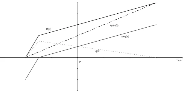
[image:11.595.145.453.129.284.2]q(a) R(a)
Figure 1: The evolution of the queue under strict queue priority with linear utility
u2(q(~a ");~a "+q(~a "));whileu1(q(a); a+q(a))<0:Hence ( )can only jump down at~a:Such a jump occurs in the linear case, where the arrival rate
is (a) = for a < ~a, and (a) = + for a > ~a, which is piecewise
constant with a downward jump at~a= + N:
Figure 1 shows the evolution of the queue under strict queue priority with linear utility. The curve R(a) is the cumulative arrival rate, the kink occurs at the time where users exit at time t = 0: The curve (t t0) represents the cumulative number of exits from the queue. The curveq(a)shows the duration in the queue for users entering the queue at timea. It is maximal for users who exit at timet :The curvea+q(a)indicates the exit time for users entering the queue
at timea:
4
No queue priority
With no queue priority, users to exit at any time are chosen at random at the rate such that all users present in the queue have the same chance to exit. We first formalize this notion and show that if there is a residual queue at the time t1 of the last arrival at the bottleneck, then the distribution of exit times conditional of being in the queue at time t1 is uniform. Using this result, we then show that the acceptable lateness condition2is sufficient to guarantee the NRQ property in Nash equilibrium under no queue priority and that the equilibrium arrival rate is indeed positive. The acceptable lateness condition cannot be relaxed in general.
probability to exit. Define the hazard rate of a user who is present in the queue at timetas
(t) = f(tja)
1 F(tja) = Q(t); (7)
wheref(tja)andF (tja)are respectively the density and cumulative distribution of exit time t conditional on being in the queue at timea: The survivor function
1 F (tja)can be expressed in terms of the integrated hazard by
1 F (tja) = e Rat (s)ds: (8)
The following technical Lemma concerns the conditional density of exit times when there is a residual queue after the last arrival. It states that when a pool of users exit with equal probability at a constant rate during some interval, then the exit time for each of them is uniformly distributed over this interval.
Lemma 2 Consider the no queue priority case. Let t1 be the time of the last
arrival and assume thatQ(t1)>0:Then the exit time conditional on being in the
queue at time a (t1 a 1)is uniformly distributed over the interval [a; 1]
withf(tja) = (a); t2[a; 1]. Furthermore, 0(a) = 2(a).
We shall now show that concave utility as defined above together with the ac-ceptable lateness condition2is sufficient to establish the no residual queue prop-erty for the no queue priority case. The acceptable lateness condition states that the marginal disutility of lateness is smaller than the marginal disutility of dura-tion in the queue. If the queue diminishes quickly enough as arrival time increases, users will then postpone arrival until the queue is no longer decreasing so quickly. The second half of the Proposition establishes that condition 2 is also necessary for the NRQ property under linear utility. Hence condition2cannot be relaxed in general.
Proposition 4 Under no queue priority, the acceptable lateness condition 2 is sufficient for the no residual queue property to hold. Under linear utility, condition
2is also necessary.
Proposition 5 establishes that the equilibrium arrival rate is always strictly positive under the acceptable lateness condition2and that the condition cannot be relaxed in general.
Proposition 5 Under no queue priority, the acceptable lateness condition 2 is sufficient for the equilibrium arrival rate to be strictly positive over the interval
[t0; t1] defined by u(0; t0) = u(0; t1). Under linear utility, condition 2 is also
Time t*
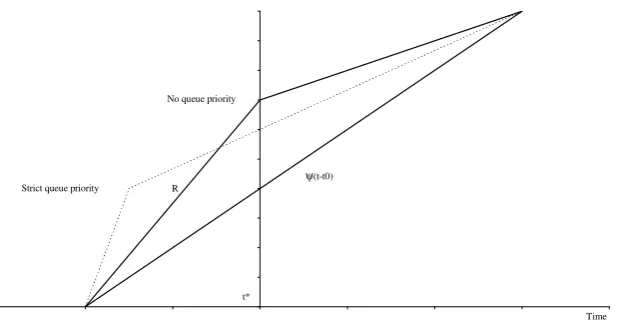
R
ψ(t-t0) No queue priority
[image:13.595.145.456.128.288.2]Strict queue priority
Figure 2: The evolution of the queue under no queue priority with linear utility
The proof of Proposition5does not guarantee existence of Nash equilibrium. However, under linear utility, the proof establishes a first-order differential equa-tion for the equilibrium arrival rate. As in the case of strict queue priority, this both gives us existence, since this arrival rate supports Nash equilibrium, and unique-ness, since any Nash equilibrium must satisfy the conditions that were used to construct the arrival rate.
Figure 2 illustrates the evolution of the queue under no queue priority and linear utility. For comparison, the figure also shows the evolution of the queue under strict queue priority. The kinked curves are the cumulative arrival rates. Note that in the NQP case, the kink in the cumulative arrival rate occurs at time
t = 0: The straight curve represents the cumulative number of exits from the
queue.
5
Loose queue priority
This section concerns the case of loose queue priority, which we shall define as an intermediate case between the cases examined so far of strict and no queue priority. As in the case of no queue priority, we cannot guarantee existence of Nash equilibrium. However, we shall show that the acceptable lateness condition
2 is sufficient to establish the no residual queue property for the case of loose queue priority; hence Condition2implies that Proposition1holds.
have a higher chance to exit than users whose present duration in the queue is shorter. So arrival time matters, even if queue priority is not strict. There are very many possibilities for explicitly defining processes that have this property. The example below provides one simple way to model loose priority.
Example 1 Introduce a variable N(a; t) denoting the number of users in the
queue at time twho arrived at the queue after timea; a t. We haveN(a; t)
Q(t): Furthermore, N(t; t) = 0 and N(t0; t) = Q(t): At time t, there are
Q(t) N(a; t) users in the queue who arrived earlier than a. Users exit the
queue at the rate ;but under loose queue priority the hazard is not the same for
everybody, it depends on the time of arrivala. We want the hazard rate, denoted
(tja);to increase with the duration of the stay in the queue. One possible way
of achieving this is by specifying the hazard rate to be
(tja) = H N(a; t)
Q(t) Q(t);
where H( ) is an increasing density on the unit interval with H(0) < 1. This
hazard rate increases with the duration in the queue. The definition
encom-passes strict and no queue priority as limiting cases as H( ) approaches
ei-ther a point mass at 1 or a uniform density. The hazard for the last user has
(tjt1) = H N(t 1;t)
Q(t) Q(t) =H(0)Q(t) < Q(t) (t1 t):
Recall that t1 is the time of the last arrival at the queue, while 1 = t1 +
Q(t1)= is the time of the last exit from the queue. When there is a residual queueQ(t1)>0then 1 > t1:
In the case of no queue priority we noted in Proposition4that the acceptable lateness condition 2implies thatQ(t1) >0 ) E(uj 1) > E(ujt1); contradict-ing that we can haveQ(t1)>0in Nash equilibrium. In this case the distribution of exit times conditional on entry at time t1 is the uniform distribution over the interval[t1; 1]:We denoted this byF (tjt1):
In the case of strict queue priority we noted that Q(t1) > 0 ) u( 1) >
u(t1);which again contradicts that we can haveQ(t1)>0in Nash equilibrium. This happens because the last user entering at time t1 will exit at time 1 with probability 1.
In order to establish the no residual queue property for the case of loose prior-ity, it is sufficient to give a condition on the distribution of exit times conditional on entry at time t1: Denote this distribution by F~(jt1): We require that loose queue priority satisfies the following condition.
is the uniform distribution over[t1; 1]with 1 =t1+Q(t1)= :
The loose queue priority condition immediately implies that if there is a resid-ual queue, then the last user to arrive is worse off under loose queue priority than under no queue priority (the utility function is decreasing in exit time, for any given arrival time). Hence Proposition4leads naturally to the following Proposi-tion.
Proposition 6 Under loose queue priority, the acceptable lateness condition 2
implies the no residual queue property in Nash equilibrium.
Hence Condition2is sufficient to ensure that Proposition1applies, also in the case of loose queue priority.
6
Concluding remarks
This paper has considered a generalized version of the Vickrey bottleneck model of congestion users having general concave utility defined over the duration in the queue as well as the time of exit from the queue. The queue may be subject to varying degrees of random sorting, ranging from strict FIFO queue priority to no queue priority. The no residual queue (NRQ) property holds when the queue has vanished at the time of the last arrival. Proposition1shows that the NRQ property is sufficient to derive a number of results that are useful for designing policies to regulate congestion. In particular, the interval of arrival as well as the expected utility of users are independent of the queueing regime, provided the NRQ prop-erty holds. The remainder of the paper then establishes that the acceptable lateness condition2, restricting the relation between the marginal utilities of duration and exit time, is sufficient for the NRQ property to hold in Nash equilibrium under all queueing regimes considered and that this condition cannot be relaxed in general. It should, however, be acknowledged that this condition is also quite restrictive. Under linear utility it rules out that a minute of lateness could be more costly than a minute of travel time. In particular it rules out that there could be a large penalty that effectively ruled out lateness.
The NRQ property is not universal. It is easy to construct straightforward cases where it does not hold. An example is strict queue priority with linear utility but with infinite cost of lateness, such that late exit is ruled out. In this case, there is a unique Nash equilibrium in which users arrive at a constant rate greater than capacity; arrivals stop at some timet1 < t and there is a strictly positive queue at this time; the queue dissipates during[t1; t ]and has vanished exactly at timet :
is behind the analyses of optimal time varying tolls in the bottleneck model, step tolls, as well as fast lane mechanisms. Common to these analyses is that they consider ways of manipulating the queue, for example by extracting revenue, that do not upset the NRQ property which ensures that the equilibrium utility is unaf-fected. Users are neutral with respect to any policy that does not affect the NRQ property. This paper has made explicit that the NRQ property underlies these in-sights and shown that it is robust within some limits to random queue sorting. It is then straightforward that, e.g., step tolling and fast laning will have similar consequences for users under random queue sorting as under strict queue priority, although they may entail different consequences for toll revenues.
For simplicity, we have only considered the case where total usageN is con-stant. The extension to endogenous total demand is however straightforward. A way to proceed is be to let aggregate demand depend on the average utility ob-tained in equilibrium; let demand be strictly increasing as a function of average equilibrium utility and assume that demand tends to0as average equilibrium util-ity tends to minus infinutil-ity. Then note that Proposition 1 states that the average equilibrium is strictly decreasing as function of the number of users. Conditional on the unique existence of Nash equilibrium for each value of N, this is suffi-cient to guarantee that Nash equilibrium exists uniquely whenN is allowed to be
endogenous. All results in the paper then generalize to the case of endogenous demand.
The paper leaves open the characterization of Nash equilibrium when the NRQ property does not hold. In that case, the convenient results of Proposition1are not available. The paper also leaves open the question of what happens under random queue sorting when the acceptable lateness condition is not satisfied. It is possible that there are combinations of queueing regimes and strictly concave utility for which the NRQ property does hold.
occurred. This property is central to the analysis of heterogeneity int under strict
References
Arnott, R. A., de Palma, A. and Lindsey, R. (1993) A structural model of peak-period congestion: A traffic bottleneck with elastic demand American
Eco-nomic Review83(1), 161–179.
Arnott, R. A., de Palma, A. and Lindsey, R. (1996) Information and usage of free-access congestible facilities with stochastic capacity and demandInternational
Economic Review37(1), 181–203.
Arnott, R. A., de Palma, A. and Lindsey, R. (1999) Information and time-of-usage decisions in the bottleneck model with stochastic capacity and demand
European Economic Review43(3), 525–548.
Arnott, R. J. (1979) Unpriced transport congestion Journal of Economic Theory
21(2), 294–316.
Barro, R. J. and Romer, P. M. (1987) Ski-Lift Pricing, with Applications to Labor and Other MarketsAmerican Economic Review77(5), 875–890.
Becker, G. S. (1991) A Note on Restaurant Pricing and Other Examples of Social Influences on PriceJournal of Political Economy99(5), 1109–1116.
Blanc, J. P. C. (2009) Bad luck when joining the shortest queueEuropean Journal
of Operational Research195(1), 167–173.
Daniel, J. I. (1995) Congestion Pricing and Capacity of Large Hub Airports: A Bottleneck Model with Stochastic QueuesEconometrica63(2), 327–370.
de Palma, A. and Arnott, R. A. (1989) The temporal use of a telephone line
Infor-mation Economics and Policy4(2), 155–174.
de Palma, A. and Fosgerau, M. (2011) Dynamic and static congestion models: a review in A. de Palma, R. Lindsey, E. Quinet and R. Vickerman (eds), A
Handbook of Transport EconomicsEdward Elgar chapter 9.
Glazer, A. and Hassin, R. (1983) ?/M/1: On the equilibrium distribution of cus-tomer arrivalsEuropean Journal of Operational Research13(2), 146–150.
Hassin, R. (1985) On the Optimality of First Come Last Served Queues
Econo-metrica53(1), 201–202.
Knudsen, N. C. (1972) Individual and Social Optimization in a Multiserver Queue with a General Cost-Benefit StructureEconometrica40(3), 515–528.
Lancaster, T. (1990) The Econometric Analysis of Transition Data Econometric
Society Monographs Cambridge University Press New York.
Lindsey, R. (2004) Existence, Uniqueness, and Trip Cost Function Properties of User Equilibrium in the Bottleneck Model with Multiple User Classes
Trans-portation Science38(3), 293–314.
Naor, P. (1969) The regulation of queue size by levying tolls Econometrica
37(1), 15–24.
Osorio, C. and Bierlaire, M. (2009) An analytic finite capacity queueing network model capturing the propagation of congestion and blockingEuropean Journal
of Operational Research196(3), 996–1007.
Sattinger, M. (2002) A Queuing Model of the Market for Access to Trading
Part-nersInternational Economic Review43(2), 533–547.
Texas Transportation Institute (2007) The 2007 Urban Mobility Report, Septem-ber.
Vickrey, W. S. (1969) Congestion theory and transport investmentAmerican
Eco-nomic Review59(2), 251–261.
Yoshida, Y. (2008) Commuter arrivals and optimal service in mass transit: Does queuing behavior at transit stops matter? Regional Science and Urban
A
Proofs
Proof of lemma1.
Proof. AllN users can arrive and be served without queueing during an interval
of lengthN= ;so 1< N= 0; 1 N= <1:There must be arrivals before the queue can start, so t0 0: Ift0 < 0, some users can benefit from postponing arrival so t0 = 0 in equilibrium. Similarly,t1 1;since otherwise some users could benefit from arriving earlier. In equilibrium, there is always queue during ] 0; 1[ since otherwise users could benefit from moving into the gap in the queue. The arrival rate is locally bounded so not all users can arrive at time0. The first arrival time occurs strictly before the preferred exit time0, since otherwise it would be possible to arrive at time 0 and be served immediately. Similarly, the last arrival time occurs strictly after time0:
Proof of Proposition1.
Proof. The NRQ property implies that t1 = 1;which means that Q(t1) = 0: Hence the durations in the queue are zero at times t0 and t1 so that u(0; t0) =
u(0; t1):By Lemma 1, the queue lasts from t0 tot1 such thatN = (t1 t0): Consequently,t0andt1are unique due to concavity ofu( )andt0 <0< t1. By the equilibrium condition, E(uja) = u(0; t0)for alla 2 [t0; t1]. Differentiating
N = (t1 t0)leads to 1 = @t@N1 @N@t0 . Differentiatingu(0; t0) = u(0; t1) leads tou2(0; t0)@t@N0 =u2(0; t1)@N@t1, so that
@t0
@N =
1 u2(0; t1)
u2(0; t0) u2(0; t1)
<0:
Then
@u(0; t0)
@N =
1 u2(0; t0)u2(0; t1)
u2(0; t0) u2(0; t1)
<0:
Straightforward computation establishes that whenu( )is concave, then the
mar-ginal utility decreases
@2u(0; t 0)
@N2 =
1
2
u2(0; t0)3u22(0; t1) u2(0; t1)3u22(0; t0)
(u2(0; t0) u2(0; t1))3
0;
with strict inequality whenu( )is strictly concave.
Proof of Proposition2.
[t0; t1]and strictly lower outside. Any other departure rate with first arrival at ^t0 would either lead to queueing or to exit later than t1;which would lead to some users achieving lower utility. Any other first arrival time than t0 would lead to utility lower thanu(0; t0);either for the first or the last user.
The following Lemma collects some relationships between the hazard rate and the corresponding conditional density and cumulative distribution function. We will use the results in the Lemma many times in the proofs below and will therefore omit references to the Lemma.
Lemma 3 Let the hazard rate and the correspondingf(tja)andF(tja)be as defined above. Then the following relations hold.
f(aja) = (a) (9)
@F(tja)
@a =
(a)
(t)f(tja) (10)
@f(tja)
@a = (a)f(tja) (11)
Proof. The first assertion follows from (7), sinceF (aja) = 0:Differentiate (8) to
find that
@F(tja)
@a = (a)e
Rt
a (s)ds = (a) (1 F (tja)):
Then the second assertion follows by substitution from (7), while the third asser-tion follows by differentiaasser-tion with respect tot:
Proof of Lemma2.
Proof. Evaluate first1 F (tja). Lett1 a t 1:Then by (8)
1 F(tja) = exp
Z t
a Q(t1) (s t1)
ds ;
where we use that Q(s) = Q(t1) (s t1): Make the substitution x =
Q(t1)= (s t1)to find that
1 F (tja) = exp
Z Q(t1)= (t t1)
Q(t1)= (a t1)
1
xdx
!
= Q(t1)= (t t1)
Q(t1)= (a t1)
Use (7) to see thatf(tja) = (a):As the density of exit times conditional ona
is constant, the exit time is uniformly distributed. To verify the last statement of the Proposition, simply differentiate
@ (a)
@a =
Q0(a)
Q2(a) = 2
Q2(a) =
2(a):
Proof of Proposition4.
Proof. Assume a Nash equilibrium with a residual queue at timet1 and consider
a > t1:The expected utility at timea;given by (2), is
E(uja) = (a)
Z 1
a
u(t a; t)dt
by Lemma2. Using the last statement of Lemma2, the derivative with respect to the arrival timeais seen to be
1 (a)
@E(uja)
@a =E(uja) u(0; a)
Z 1
a
u1(t a; t)dt: (12)
Considering the following identity
u( 1 a; 1) u(0; a) =
Z 1
a
[u1(t a; t) +u2(t a; t)]dt;
we may write
1 (a)
@E(uja)
@a =E(uja) u( 1 a; 1) +
Z 1
a
u2(t a; t)dt:
Add the two expressions for @E(uja)
@a to obtain
1 (a)
@E(uja)
@a = E(uja)
1
2(u(0; a) +u( 1 a; 1))
+ 1
2
Z 1
a
[u2(t a; t) u1(t a; t)]dt
The first term on the RHS is positive by Jensen’s inequality since u(t a; t)is concave as a function oftand the second term is strictly positive by Condition2:
Thus,E(uja)is strictly increasing on]t1; 1[so that
which contradicts Nash equilibrium.
To verify the second assertion of the Proposition, note that in the linear case,
1 (a)
@E(uja)
@a =
1 2
Z 1
a
[u2(t a; t) u1(t a; t)]dt
= 1
2( 1 a) ( ):
Then @E(uja)
@a >0is equivalent to Condition2and so Condition2is also necessary.
Proof of Proposition5.
Proof. The expression for the expected utility conditional on arrival at time ais
(2). Using (11), we express the equilibrium condition for the no queue priority case as follows.
@E(uja)
@a = (a)E(uja) u(0; a) (a) E(u1ja) = 0;
which can be solved using (a) = =Q(a)to yield
Q(a)
= E(uja) u(0; a)
E(u1ja)
:
Differentiate again and use that (1) givesQ0(a) = (a) to find
(a)
= 1 u2(0; a)
E(u1ja)
@E(u1ja) @a
(a)E(u1ja)
: (14)
Multiply all terms in (14) by (a)E(u1ja)>0to find that (a)>0iff
(a)E(u1ja) + (a)u2(0; a) +
@E(u1ja)
@a >0: (15)
Carry out the differentiation using Lemma3to find that
@E(u1ja)
@a = (a)u1(0; a) E(u11ja) + (a)E(u1ja):
Insert this into the inequality (15) to find that it is equivalent to
The second term is positive sinceuis concave:Therefore Condition2implies that
(a)>0.
When utility is linear, (14) shows that the equilibrium arrival rate is
(a) =
+ ; a <0
; a >0:
Then (a)>0implies Condition2.
Proof of Proposition6.
Proof. Assume that Q(t1) > 0. ThenEF~(ujt1) EF (ujt1), due to first-order stochastic dominance. But EF(ujt1) < u(0; 1) by (13) in the proof of Propo-sition 4. Then EF~(ujt1) < u(0; 1) and the last user would prefer to arrive at 1 rather than at t1: This contradicts Nash equilibrium. Hence we must have