Munich Personal RePEc Archive
A note on implementing the Durbin and
Koopman simulation smoother
Jarocinski, Marek
European Central Bank
24 October 2014
Online at
https://mpra.ub.uni-muenchen.de/59466/
A note on implementing the Durbin and Koopman
simulation smoother
Marek Jaroci´
nski
∗October 24, 2014
Abstract
The correct implementation of the Durbin and Koopman simulation smoother is explained. A possible misunderstanding is pointed out and clarified for both the basic state space model and for its extension that allows time-varying intercepts (mean adjustments).
Keywords: state space model; simulation smoother; trend output (JEL: C3; C15)
1
Introduction
Consider the state space model
yt=Ztαt+εt, εt ∼N(0, Ht) (1a)
αt+1 =Ttαt+Rtηt, ηt∼N(0, Qt), t = 1, ..., T, and (1b)
α1 ∼N(a1, P1), (1c)
where yt is the observation vector, αt is the unobserved state vector, and εt and ηt are vectors of disturbances uncorrelated at all lags. The matrices Zt, Ht, Tt, Rt, Qt, P1 and
vector a1 are assumed to be known. For further details and illustrations of this model
see, e.g., Durbin and Koopman (2012).
This note explains the implementation of the Durbin and Koopman (2002) simula-tion smoother for this model, pointing out a possible misunderstanding. A simulasimula-tion
∗European Central Bank, Kaiserstrasse 29, 60311 Frankfurt am Main, Germany, e-mail:
smoother is an algorithm for drawing the states α = (α′
1, ..., α′T)′, or the disturbances
(ǫ′
1, η1′, ..., ǫ′T, ηT)′, from their distribution conditional on the observables y = (y1′, ...yT′ )′.
The misunderstanding may arise when drawing the states. It does not arise when drawing the disturbances.
2
The correct implementation
This section explains how to implement Durbin and Koopman’s approach to drawing α conditional on y in the model (1a-1c). Let us call this algorithm ‘Algorithm 2a’ to differentiate it from their Algorithm 2.
Algorithm 2a. (modified from Durbin and Koopman (2002) Algorithm 2, p.607) Step 1. Draw α+
and y+
by means of recursion (1a-1b), where the recursion is initial-ized by a draw α+
1 ∼N(0, P1).
Step 2. Construct the artificial series y∗ = y−y+
and compute αˆ∗ = E(α|y∗) by
putting y∗ through the Kalman filter and smoother.
Step 3. Take α˜= ˆα∗+α+
. α˜ is a draw from the distribution of α conditional on y.
An alternative implementation of this algorithm, which is also correct, uses (1a-1c) for the simulation of y+
, α+
in Step 1 but then uses the model with α1 ∼ N(0, P1) to
compute the conditional expectation ˆα∗ =E(α|y∗) in Step 2.
The value added of this note lies in stating the above algorithm explicitly and in particular, in pointing out that a1 needs to be reset to 0, i.e., the initial condition α1 ∼
N(a1, P1) (1c) needs to be replaced byα1 ∼N(0, P1) either in Step 1 or in Step 2. Durbin
and Koopman (2002) state Algorithm 2, which is slower, and only suggest Algorithm 2a informally without stating it explicitly. In particular, they do not warn the reader that a1 should be reset to 0 either in Step 1 or in Step 2, which gives rise to a possible
misunderstanding that the unmodified model (1a-1c) can be used both in Step 1 and in Step 2.
Two conditions have a potential to render the above misunderstanding immaterial.
1. Diffuse initialization. Durbin and Koopman (2002) prove in their Appendix 2 that the diffuse elements ofα1+ can be set equal to arbitrary quantities, hence the values
of a1 corresponding to these elements do not matter.
2. Zero mean. For the elements of α+1 that have a zero mean the correction obviously
Therefore, the misunderstanding is immaterial when all the elements of α1 are either
diffuse or have a zero mean.
In a model with intercepts another modification of Algorithm 2 is needed. Suppose the model is given by (1c),
yt =dt+Ztαt+εt, εt∼N(0, Ht) and (2a)
αt+1 =ct+Ttαt+Rtηt, ηt ∼N(0, Qt), (2b)
wheredt and ct are intercepts that are known and may change over time. The remaining
quantities are defined under equations (1a-1c). Algorithm 2a can also be used with this model, but the interceptsdt andctshould be reset to 0 for allt either in Step 1 or in Step
2.
3
A formal justification
I now provide a formal justification of Algorithm 2a. This algorithm assumes
α y ! ∼N µα µy !
, Σαα Σαy Σαy Σyy
!! and α + y+ ! ∼N 0 0 !
, Σαα Σαy Σαy Σyy
!!
, (3)
where the unconditional moments µα, µy, Σαα, Σαy and Σyy are functions of Zt, Ht, Tt,
Rt,Qt,P1,a1 (ct, dtif applicable) implied by (1a-1c) or by (2a,2b,1c). Note, in particular,
that resetting of µα and µy to 0 is achieved by resetting a1 and, if applicable, ct and dt
for all t to 0.
A draw ˜α is generated as
˜
α=E(α|y∗) +α+
=µα+ ΣαyΣ−
1
yy(y−y
+
−µy) +α
+
.
The first and second moments of ˜α conditional on y are
E(˜α|y) =µα+ ΣαyΣyy−1(y−µy) = E(α|y) and
V(˜α|y) = ΣαyΣ−
1
yyΣyyΣ−
1
yyΣ′αy −2ΣαyΣ−
1
yyΣ′αy + Σαα = Σαα−ΣαyΣ−
1
yyΣ′αy =V(α|y).
Hence, the first and second moments of ˜αare correct and ˜α is indeed a draw fromp(α|y). Note, however, that setting the mean of (α+
, y+
) to (µα, µy) due to the discussed
4
Numerical examples
I illustrate the effect of the possible misunderstanding using two numerical examples from the literature.
4.1
Nile data
The first example is the well-known local level model of the Nile data (a series of readings of the annual flow volume at Aswan from 1871 to 1970). Durbin and Koopman (2012), and others fit the following model to these data:
yt=αt+εt, εt ∼N(0,15099) and (4a)
αt+1 =αt+ηt, ηt∼N(0,1469.1), (4b)
where y is the observed flow volume andα is its unobserved trend.
Table 1 reports the means and standard deviations of 10,000 draws of the trend α generated with several setups. “Initialization 1” assumes, for illustrative purposes, that α1 comes from the Gaussian distribution centered at the first observation y1 with the
variance equal to the variance of the deviations of α from y throughout the sample, i.e. 15099. I generate 10,000 draws using Algorithm 2a and then I generate 10,000 draws with an incorrect variation of this algorithm, where I do not reset a1 to 0 neither in Step
1 nor in Step 2. It is clear from Table 1 that the misunderstanding seriously distorts the simulation smoother: the mean of the trend in the first period, α1, is 1114 with the
correct algorithm (column 1) and 1350 with the incorrect variation (column 2). After 50 periods the initialization matters less and the means of the trend in period 50, α50,
obtained with Algorithm 2a and its incorrect variation are similar, 834 vs 835. Then I use the diffuse initialization for α and generate 10,000 draws first with Algorithm 2a and then with its incorrect variation. When the initialization is diffuse I obtain the same means and standard deviations ofαwith both implementations of Algorithm 2a, so I only report them once (column 3). To summarize, this numerical example illustrates that the misunderstanding can distort the results significantly 1) for the draws of states in the beginning of the sample and 2) when the initialization of the state is non-diffuse.
4.2
Trend of real GNP
Table 1: Trend flow volume in the Nile model. Mean, standard deviation in parenthesis. Initialization 1 (non-diffuse) Diffuse initialization
Algorithm 2a No resetting of a1
τ1 1112 (57) 1350 (57) 1111 (64)
τ50 834 (48) 835 (49) 835 (48)
from 1949 to 1984.
yt =τt+ςt, (5a)
τt = 0.008 +τt−1+ηtτ, ηtτ ∼N(0,0.0057 2
) and (5b)
ςt = 1.501ςt−1−0.577ςt−2+ηtς, ηtς ∼N(0,0.0076 2
), (5c)
where τt is a trend and ςt is a cycle, both unobservable.
Table 2 reports the mean and standard deviation of 10,000 draws of trend GNP, generated with several setups. “Initialization 1” assumes that ς1 comes from the ergodic
distribution of ςt and that τ1 is centered at the last value of GNP before the start of
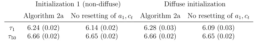
the sample, with the ergodic variance of ςt. This is a natural assumption exploiting the stationarity of ςt. I generate 10,000 draws using Algorithm 2a and then I generate 10,000 draws with an incorrect variation of this algorithm, where I do not reset a1 and ct
to 0 neither in Step 1 nor in Step 2. It is clear from Table 2 that the misunderstanding seriously distorts the simulation smoother: the mean of the trend GNP in the first period, τ1, is 6.24 with the correct algorithm (column 1) and 6.14 with the incorrect variation
(column 2). After 50 quarters the initialization matters less and the means of the trend GNP in period 50, τ50, obtained with Algorithm 2a and its incorrect variation are the
similar, 6.66 vs 6.65. Next, I use the diffuse initialization of τ and ς. The mean of τ1 is
6.28 with Algorithm 2a (column 3) and 6.09 with its incorrect variation (column 4). The misunderstanding matters here even with the diffuse initialization of τ and ς, because when model (5a-5c) is cast in form (1a-1b) the constant term of equation (5b) is a state with a non-zero and non-diffuse initialization and the failure to reset a1 to 0 distorts the
simulation smoother. Equivalently, when model (5a-5c) is cast in form (2a-2b) all the states are zero-mean or diffuse, but the failure to reset ct to zero distorts the simulation
Table 2: Trend GNP in Watson’s model based on simulation smoothers. Mean, standard deviation in parenthesis.
Initialization 1 (non-diffuse) Diffuse initialization
Algorithm 2a No resetting ofa1, ct Algorithm 2a No resetting of a1, ct
τ1 6.24 (0.02) 6.14 (0.02) 6.28 (0.03) 6.09 (0.03)
τ50 6.66 (0.02) 6.65 (0.02) 6.66 (0.02) 6.65 (0.02)
5
Conclusion
This note explains the implementation of the Durbin and Koopman algorithm for drawing the states conditionally on the observables in a state space model, pointing out a possible misunderstanding. The misunderstanding matters when the initial state vector is not all zero-mean or diffuse, or when a nonzero intercept is present, and leads to incorrect draws of the states, especially in the beginning of a sample. By clarifying the possible misunderstanding, this note hopefully encourages an even wider use of the Durbin and Koopman algorithm by practitioners.
References
Durbin, J. and Koopman, S. J. (2002). A simple and efficient simulation smoother for state space time series analysis. Biometrika, 89(3):603–615.
Durbin, J. and Koopman, S. J. (2012). Time Series Analysis by State Space Methods: Second Edition. Oxford Statistical Science Series. OUP Oxford.