1
Statistical model specification and power: recommendations on the use of test-qualified pooling in 1
analysis of experimental data 2
3
Nick Colegrave1 and Graeme D Ruxton2 4
1. School of Biological Science, University of Edinburgh, Edinburgh EH14 4AJ, UK 5
2. School of Biology, University of St Andrews, St Andrews KY16 9TH, UK 6
Abstract 7
A common approach to the analysis of experimental data across much of the biological sciences is 8
test-qualified pooling. Here non-significant terms are dropped from a statistical model, effectively 9
pooling the variation associated with each removed term with the error term used to test 10
hypotheses (or estimate effect sizes). This pooling is only carried out if statistical testing on the basis 11
of applying that data to a previous more complicated model provides motivation for this model-12
simplification; hence the pooling is test-qualified. In pooling, the researcher increases the degrees of 13
freedom of the error term with the aim of increasing statistical power to test their hypotheses of 14
interest. Despite this approach being widely adopted and explicitly recommended by some of the 15
most widely-cited statistical textbooks aimed at biologists, here we argue that (except in highly 16
specialised circumstances that we can identify) the hoped-for improvement in statistical power will 17
be small or non-existent, and there is likely to be much reduced reliability of the statistical 18
procedures through deviation of type I error rates from nominal levels. We thus call for greatly 19
reduced use of test-qualified pooling across experimental biology, more careful justification of any 20
use that continues, and a different philosophy for initial selection of statistical models in the light of 21
this change in procedure. 22
2 Introduction
24
A common approach to the analysis of experimental data across disparate parts of the biological 25
sciences is test-qualified pooling. A common manifestation of this approach can be summarised as 26
follows: the researcher fits their data to a model that they select on the basis of the design of their 27
study and the hypotheses they are interested in testing. After examining the significance of terms in 28
the model that are not specifically related to the hypothesis currently under investigation, the 29
researcher then removes non-significant terms from the model, and re-fits their data to this 30
simplified model. That is, some terms were included in the original model not because they allow an 31
interesting hypothesis to be tested but because (on the basis of the specifics of the experimental 32
design allied to previous knowledge of the system) they were expected to explain substantial 33
portions of the variation. If the data generated in this particular experiment do not suggest that one 34
or more of these terms are strongly influential then they are dropped from the model, and further 35
analysis is performed based on a simplified model. Such a simplification process is often seen as 36
attractive in making presentation of results more compact, in highlighting more influential variables, 37
and/or in increasing statistical power for exploring the significance of remaining terms. By 38
simplifying the model in this way, the researcher is effectively pooling the variation associated with 39
each removed term with the error term that will ultimately be used to test their hypotheses. This 40
pooling is only carried out if statistical testing on the basis of applying that data to a previous more 41
complicated model provides motivation for this approach, hence the pooling is test-qualified. In 42
pooling, the researcher increases the degrees of freedom of the error term with the aim of 43
increasing statistical power to test their hypotheses of interest. Despite this approach being widely 44
adopted and explicitly recommended by some works on data analysis (e.g. [1]), other influential 45
authors explicitly warned against this practice (e.g. [2]). Here we want to offer some resolution of 46
this apparent conflict in the literature, in order to help authors, reviewers, editors and readers 47
evaluate the consequences of pooling in different circumstances. Note that although we couch this 48
3
approaches based on estimation of effect size; our discussion is however focussed on the analysis of 50
data from planned experiments rather than from purely observational studies. The costs and 51
benefits of test-qualified pooling are more clear-cut for planned experiments where potential 52
confounding factors can often be eliminated or controlled for by careful experimental design, 53
removing the need to deal with these factors statistically. Also, planned experiments generally are of 54
what is termed a “confirmatory” nature, where the study specifically aims to test one or more 55
hypotheses known from the outset. Observational studies more often have an “exploratory” 56
motivation involving measuring a broad range of variables and then seeking to rank them in terms of 57
potential importance and influence. We return to these issues in the Discussion. 58
Being clear what pooling is and why you might want to do it 59
To clarify the issues we consider a specific example. You are interested in the effect of an 60
experimental treatment (a new humidification system) on the growth of individually-potted tomato 61
plants. Your experiment will be conducted in ten small greenhouses at your research station, and the 62
nature of the treatment means that it has to be applied to whole greenhouses. You install the 63
humidification system in five (randomly selected) greenhouses, leaving the other five as controls, 64
and you assay the growth of 40 tomato plants in each greenhouse. In this design the greenhouse is 65
the experimental unit, and any hypothesis test of the treatment should use an error based on the 66
variation amongst greenhouses rather than variation amongst the individual plants. In this case the 67
simplest means of analysis would be to calculate a mean growth rate across the 40 plants in each 68
greenhouse and carry out a one-way ANOVA using these 10 independent data points. 69
However, as a thought experiment, suppose that we somehow knew for a fact that growth 70
conditions (in the absence of our treatment manipulation) were absolutely identical amongst our 71
greenhouses. In this imaginary situation we might argue that, since greenhouse-to-greenhouse 72
variation is not confounded with any treatment effect we can use the growth measures from the 73
4
in our degree of freedom, and consequently our statistical power to detect treatment effects. Of 75
course in reality, we cannot usually know with certainty whether our greenhouses vary, and this has 76
led to the development of methods for test-qualified pooling. In this case, we would start by fitting 77
the nested model defined by the design of our study (with individual plants being nested within 78
greenhouse). This would include the treatment term, a nested term for the variation amongst 79
greenhouses in the same treatment group, and a second error term corresponding to the variation 80
amongst plants in the same greenhouse. The key to test-qualified pooling is that the set of data itself 81
influences the nature of the analyses performed on it. If initial analysis of the full model indicates 82
substantial variation amongst greenhouses, then the significance of the treatment term is tested 83
using the variation amongst greenhouses as its error term with 8 df. However, if there is no evidence 84
of substantial greenhouse-to-greenhouse variation in this initial analysis then the among-85
greenhouse and the true error variations are pooled, and this combined error term with 398 df is 86
used then to provide a test of the treatment effect that is expected to benefit from higher statistical 87
power (see [3-5] for commonly-cited texts that recommend this approach). The justification that 88
advocates of test-qualified pooling give for this approach is that in the absence of any greenhouse 89
effect, the among-greenhouse and the within-greenhouse error terms are both estimating the same 90
thing, and so by combining them we get a better estimate than we would estimating the two 91
separately. 92
However pooling is not limited to nested designs. Continuing with tomatoes and greenhouses, you 93
now want to compare the effects of four different growing media in individually-potted tomato 94
plants rather than the effect of humidity. To gain a sufficient sample size for the experiment you 95
have to use three different greenhouses to keep all the plants, but because your treatments can now 96
be applied randomly to individual plants, you randomly allocate equal numbers of plants to each 97
treatment in each greenhouse leading to a randomised block design (with specific greenhouse 98
identity as the blocking factor, with three levels). The statistical model implied by this design would 99
5
as well as a treatment-by-greenhouse interaction and an amongst-plant error term based on the 101
variation amongst individual plants within the same treatment-greenhouse combination. Depending 102
on the exact hypothesis we wish to test, the appropriate error term for our treatment effect will be 103
either the interaction term, or the amongst-plant error term [6], but in either case, if the interaction 104
term is not significant, we might chose to pool its variation with the amongst-plant error term prior 105
to testing the treatment effect. Similarly, we might then decide that if the greenhouse term is also 106
non-significant, we would add that source of variation and its associated degrees of freedom to our 107
error pool. In either case, we would be carrying out test-qualified pooling. 108
Another form of pooling can involve the initial test that triggers whether pooling is used or not being 109
entirely separate to the model testing the hypotheses of interest. To illustrate this, we return to the 110
experiment above comparing the effects of four different growing media on individually-potted 111
tomato plants. Imagine that, because of a change of supplier at your institute, you ended up using 112
two different but broadly similar types of pots to grow the tomatoes in. Plants are randomised to 113
pot type as well as to growth medium and greenhouse. You really do not expect type of pot to 114
influence growth rates, but just to be careful you first of all perform a t-test comparing growth rates 115
across the two types of pot. Your plan is that if (as you expect) this t-test reveals no evidence of a 116
difference, you report this and use this test as justification for pooling data across the two pot types 117
in your subsequent analyses. However if it does reveal evidence of a difference then you will either 118
add pot-type as a factor in subsequent analyses or carry out separate analyses for the two types of 119
pot. Again, there is the potential for pooling driven by the results of a pre-test, so this scenario is 120
another manifestation of test-qualified pooling. 121
Why is test-qualified pooling controversial? 122
The case against pooling was made most forcefully and explicitly in the biological literature by Stuart 123
Hurlbert primarily in relation to its use in nested designs [2]. Hurlbert coined the expression 124
6
they were independent in their data analysis. His original paper on this [7] has been cited over 6000 126
times and has been hugely influential in the design of data collection and the analysis of data 127
spanning all of biology. Hurlbert considers the pooling of errors in a nested analysis to be a form of 128
pseudoreplication, a form that he calls test-qualified sacrificial pseudoreplication. He argues that 129
pooling biases p-values downwards and biases confidence intervals towards being too narrow. He 130
further argues that demanding a higher p-value than 0.05 in the initial test before pooling (a process 131
often called “sometimes pooling”) reduces but does not eliminate these problems. An analogous 132
argument can be made against pooling interaction terms with error terms when analysing 133
randomised block designs [6]. However, even in situations where pooling might not be regarded as 134
analogous to pseudoreplication (e.g. pooling an interaction between two fixed factors prior to 135
testing the main effects), type 1 error rates can be increased (as we will see below). Despite this, 136
pooling is still regularly practiced, and is recommended in influential statistics textbooks aimed at 137
biologists (e.g. [3-5]) and research papers on statistical methodology (e.g. [2,8] ). In the next section 138
we argue that both philosophically and pragmatically there are strong arguments for siding with 139
Hurlbert. 140
The philosophy and pragmatics of pooling 141
The two main philosophical arguments against pooling are well articulated by Newman et al. [7], and 142
can be explained in the context of our greenhouses and growth media example. Firstly, if we use 143
pooling, then the way that we test for an effect of growth medium becomes conditional on the data, 144
but that conditionality is not acknowledged in the associated p-values. That is, whether we test the 145
effect of medium in a model with or without a greenhouse term will be determined by the data. 146
Philosophically, p-values are probabilities based on a very large number of notional replicates of 147
exactly the experiment under investigation. So imagine that we repeat the full experiment and 148
analysis of the resulting data again and again. In replicates of this experiment, if we adopt a test-149
7
sometimes the other. For each form of the analysis, that particular analysis will be implemented only 151
for a specific subset of replicate experiments determined by the patterns of data in that replicate 152
experiment. Importantly, this is a biased sample of all the possible replicate experiments in terms of 153
properties of the sample. Yet the test is predicated on the assumption that it is applied to data from 154
an experiment drawn without bias from the population of all possible replicates of this experiment. 155
It is this mismatch that leads to lack of control of type I error and of confidence intervals. Secondly, 156
by pooling (no matter what critical value we compare the calculated p-value against) we are 157
accepting that the null hypothesis that there is no effect of greenhouse is true, and the whole 158
philosophy of null-hypothesis statistical testing is that the null hypothesis is never accepted as true, 159
rather we might either reject it or find that we do not have sufficient grounds to reject it. Thus, from 160
a purist philosophical perspective pooling should not be recommended. 161
We next ask if there is a pragmatic argument that says that pooling may have some less-than-ideal 162
properties, but pooling leads to relatively mild misbehaviours that are sometimes outweighed by the 163
(enhanced power) benefits of pooling. There is no underlying theory to give general and definitive 164
answers to the issue of pragmatics raised above; all we have to go on are a number of numerical 165
explorations of specific cases. However, the consensus in this literature is that (i) pooling can cause 166
actual type one error rates to be very different from the nominal value, and (ii) there is no consistent 167
and substantial increase in power to compensate. Walde-Tsadik & Afifi [9] explore the effect of 168
always pooling when one factor is associated with a p-value above 0.05, and also of “sometimes 169
pooling” when the required critical value was higher than 0.05 in two-way ANOVA random effects 170
models. They found that both procedures very rarely offered adequate control of type-1 error rate 171
and even less commonly lead to significant improvement in power to test for an effect of the other 172
factor. Hines [10] performed extensive simulations and concluded that for multifactorial ANOVA 173
“the conditions for pooling to be even potentially rewarding are more restrictive than might be 174
expected, and power improvements are generally lower”. Janky [11] performed a similar analysis of 175
8
insubstantial gain in power (and often power loss) relative to the nominal test.” Even when using a 177
conservative “sometimes pooling” value of = 0.35 to trigger pooling, Janky found the type I error 178
rate in subsequent tests on pooled data rose from the nominal 5% to generally somewhere between 179
7% and 11%. This study was interesting for highlighting that pooling actually led to a reduction of 180
power more often than it lead to a substantial gain in power; this occurs because the increase in 181
inherent variation caused by pooling dominates any effect of increased degrees of freedom devoted 182
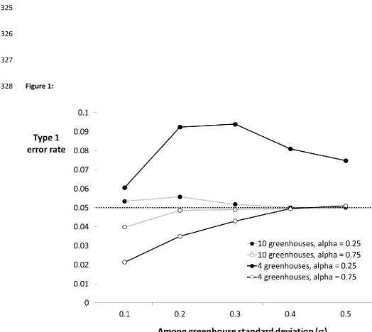
to exploring remaining factors. Figure 1 shows examples of deviations in both directions from the 183
nominal 5% level for type I error rates generated by simulations of our whole-greenhouse-treatment 184
thought experiment. In exploring our model we found that small changes in parameter values could 185
lead to substantial change in the magnitude and direction of deviations from the nominal level. It is 186
difficult to make generalisations about the circumstances under which deviations will be strongest. 187
In common with the other studies discussed directly above, we found that the direction and 188
magnitude of deviations are driven by a complex interaction between structure of the experimental 189
design, aspects of the shape of the underlying “population” from which sample values are obtained, 190
and sample sizes. Also, as the highest line in Figure 1 illustrates, relationships with parameter values 191
can be non-monotonic. 192
Discussion and Conclusion 193
Use of test-qualified pooling is widely adopted, but its prevalence across biological sciences is 194
patchy. For example, it is much less commonplace in clinical trials; where often statistical analyses 195
have to be specified in pre-registration of trials, and thus scope for flexibility in data analysis is 196
reduced. Test-qualified pooling is also relatively uncommon in the agricultural sciences, where 197
particular designs and modes of analysis that avoid issues of pooling are traditional; and the 198
statistical software package Genstat is commonly used, which is particularly suited to forms of 199
9
We do still consider that test-qualified pooling is over-used in biology. Simply, in “confirmatory 201
studies” based on designed experiments where we aim to test specific hypotheses (or estimate 202
specific effect sizes) we do not recommend pooling under any circumstances. The often-modest 203
expected increases in power from pooling do not make it an attractive option when its drawbacks 204
are taken into account. Apart from statistical power, the other attraction to pooling is simplification 205
of the presentation of results, but we feel that this will never be sufficient grounds for justifying the 206
process. We would only recommend pooling in such a study if the decision to consider test-qualified 207
pooling was made on the basis of a prior simulation study that aimed at evaluating the 208
consequences of pooling for Type I and Type II error rates. We have yet to see an example of a study 209
that provided such a justification for pooling. 210
As we mentioned in the Introduction, it is not as easy to offer clear and simple guidance on pooling 211
in purely observational studies, and studies where the researchers’ aims are more focussed on 212
exploration or prediction than on testing specific hypotheses. However, in such situations pooling 213
can be seen as a facet of model selection – which is an area of considerable activity in applied 214
statistics. A particularly useful introduction to the concepts involved is that of Chatfield [12]. He 215
makes the point that if the same data-set is used to both select the most appropriate model from a 216
suite of alternatives and also to fit that model, then the interpretation of the fitted model should be 217
quite different from circumstances where the form of the model is decided upon first and only then 218
is the data applied to fit that model. Where there is uncertainty as to the most appropriate model, 219
then there are methodological developments in model averaging that can acknowledge this ([13] 220
and [14] offer good introductions for the biologist). A failure to properly acknowledge model 221
uncertainty when the same data is used to select and fit the model can read to very unreliable 222
inferences ([12],[15],[16]). 223
Despite the complexity of the literature on model selection and model uncertainty, we feel that we 224
10
more exploratory studies where the intention is to identify factors that might be of interest, rather 226
than to test specific hypotheses, then test-qualified pooling might be more attractive; since 227
researchers may be willing to live with loss of control of type I error rates if this helps boost their 228
statistical power to flag up factors of interest. That is, they may be prepared to suffer higher rates of 229
false positives to boost their likelihood of detecting real effects. We expect that these power gains 230
may sometimes be considerable for nested-designs. However for other types of design the literature 231
discussed in the last section should serve as a caution that power gains from pooling may be small or 232
non-existent. Our view is that even in exploratory studies, test-qualified pooling cannot really be 233
recommended except perhaps where the design is nested and where the size of the experiment was 234
reduced from its ideal size by practical constraints or unforeseen adverse circumstances. 235
Where does this leave the experimenter in our tomato plant example who just wanted to be diligent 236
and reassure themselves and their readers that there was no effect due to two different types of 237
pots being used? They have to make a decision about how important this check is to them. If they 238
feel that it is worth investing a few degrees of freedom in, then they should include type-of-pot as a 239
factor in their analysis and pay a modest cost in reduced power to test the hypothesis (comparing 240
different growth media) that they are really interested in. Alternatively, they may decide that careful 241
experimental design and explanation of that experimental design should allay concerns about 242
differential effects of pot types sufficiently that there is no need for formal statistical testing. More 243
generally, we all have to accept that there are no free statistical analyses, and think hard about 244
which factors to include in any model. This is analogous to the decision to block on a given variable 245
in experimental design. It is only advantageous to block on variables that explain a substantial 246
fraction of variation between experimental units, otherwise the degrees of freedom lost in including 247
that blocking term are not compensated for by effective partitioning of variation into error and other 248
11
Sometimes we can make a strong enough case based on careful experimental design (especially use 250
of randomisation), biological intuition, and logical reasoning for why we can safely assume that some 251
potentially influential factors are in fact very unlikely to be important in our study, and so we omit 252
them from our statistical procedures. In fact, we do this all the time. In our example the researcher 253
felt no need to test whether which shelf on a greenhouse a pot was placed on had an effect, or what 254
side of the greenhouse, or how near to the door of the greenhouse it was. Sometimes we will feel 255
that we cannot make a sufficiently strong case this way, and we should then include that factor in 256
our model and explore its effects statistically. As so often in the design and analysis of scientific 257
studies, there are no black-and-white rules for which factors to include in your statistical model; we 258
need to think hard about it and justify our choices in terms of experimental design, understanding of 259
underlying biology and logical reasoning. This should be good news: model selection should be much 260
more about biology than about mathematics and probability theory – and biology is what we are 261
interested in. 262
Acknowledgment: We thank Gavin Gibson and three anonymous reviewers for perceptive 263
comments. 264
Author contributions: This article was conceived, developed and written equally by both authors. 265
References 266
[1] Schank, J. C., & Koehnle, T. J. (2009). Pseudoreplication is a pseudoproblem.Journal of 267
Comparative Psychology, 123(4), 421.
268
[2] Hurlbert, S. H. (2009). The ancient black art and transdisciplinary extent of
269
pseudoreplication. Journal of Comparative Psychology, 123(4), 434.
270
[3] Sokal, R. R., & Rohlf, F. J. (1995). Biometry: the principals and practice of statistics in biological
271
research. WH Freeman and Company, New York.
272
[4] Quinn, G. P., & Keough, M. J. (2002). Experimental design and data analysis for biologists.
273
Cambridge University Press.
12
[5] Zar, J. H. (1999). Biostatistical analysis. Pearson Education India.
275
[6] Newman, J. A., Bergelson, J., & Grafen, A. (1997). Blocking factors and hypothesis tests in
276
ecology: is your statistics text wrong?. Ecology, 78(5), 1312-1320.
277
[7] Hurlbert, S. H. (1984). Pseudoreplication and the design of ecological field experiments. Ecological 278
monographs, 54(2), 187-211.
279
[8] Crits-Christoph, P., Tu, X., & Gallop, R. (2003). Therapists as fixed versus random effects-some
280
statistical and conceptual issues: a comment on Siemer and Joormann (2003).Psychological Methods
281
8, 518-523.
282
[9] Wolde-Tsadik, G., & Afifi, A. A. (1980). A comparison of the “sometimes pool”,“sometimes switch”
283
and “never pool” procedures in the two-way ANOVA random effects model. Technometrics, 22(3),
284
367-373.
285
[10] Hines, W. G. S. (1996). Pragmatics of pooling in ANOVA tables. The American Statistician, 50(2),
286
127-139.
287
[11] Janky, D. G. (2000). Sometimes pooling for analysis of variance hypothesis tests: A review and
288
study of a split-plot model. The American Statistician,54(4), 269-279.
289
[12] Chatfield, C. (1995). Model uncertainty, data mining and statistical inference. Journal of the Royal 290
Statistical Society, Series A, 158, 419–466. 291
[13] Whittingham, M. J., Stephens, P. A., Bradbury, R. B. & Freckleton, R. P., (2006). Why do we still
292
use stepwise modelling in ecology and behaviour?. Journal of Animal Ecology, 75,.1182-1189.
293
[14] Richards, S. A., Whittingham, M. J. & Stephens, P. A., (2011). Model selection and model
294
averaging in behavioural ecology: the utility of the IT-AIC framework. Behavioral Ecology and 295
Sociobiology, 65, 77-89.
296
[15] Blanchet, F. G., Legendre, P. & Borcard, D., (2008). Forward selection of explanatory
297
variables. Ecology, 89, 2623-2632.
13
[16] Mundry, R. & Nunn, C. L., (2009). Stepwise model fitting and statistical inference: turning noise
299
into signal pollution. The American Naturalist, 173, 119-123.
300
301
302
Figure legend 303
Figure 1: To illustrate how the type 1 error rate can be affected by test qualified pooling we 304
examined simulated data sets for both 4 (broken line) and 10 (solid line) greenhouses. In both cases, 305
equal numbers of greenhouses were allocated to control or treatment conditions (but condition had 306
no effect on plant growth), and 40 plants were measured in each greenhouse. We also examined the 307
effect of two different alpha levels for the pooling decision (recommended in [3]: open circles = 0.25 308
and closed circles = 0.75), and several different levels of among-greenhouse variation (). Under
309
many different parameter combinations the actual type 1 error rate differs from the desired value of 310
0.05, sometimes substantially. 311
Plant growth rates were calculated as a baseline value (10) plus an individual deviation drawn from 312
N(0,1) plus a greenhouse-deviation drawn from N(0,) and the same for all plants in a given 313
greenhouse. We analysed each data set in two ways. First we carried out a nested analysis of 314
variance in which the treatment mean square was tested over the among-greenhouses within-315
treatment mean square. The same analysis tested for variance among greenhouses by comparing 316
the among-greenhouses mean square to the amongst-plants error mean square. Second we carried 317
out an analysis in which data from all greenhouses was pooled. The decision as to which P value to 318
use for our actual hypothesis test for the effect of the treatment was based on the significance of 319
the among-greenhouse test at one of two alpha levels. If this test was significant at the appropriate 320
alpha level we used the P value from the nested model, otherwise we used the P value from the 321
14
of less than 0.05 (i.e. a false positive at alpha = 0.05) is an estimate of the type 1 error rate. The 323
simulations were carried out in R, with the AOV function being used for the analyses. 324
325
326
327
Figure 1: 328
[image:14.595.36.561.132.600.2]