Solving Large Scale Unconstrained Minimization Problems by a New ODE Numerical Integration Method

doi:10.4236/am.2011.25069 Published Online May 2011 (http://www.SciRP.org/journal/am)

Solving Large Scale Unconstrained Minimization Problems

by a New ODE Numerical Integration Method

Tianmin Han1, Xinlong Luo2, Yuhuan Han3

1

China Electric Power Research Institute, Beijing, China

2

School of Information and Communication Engineering, Beijing University of Posts and Telecommunications, Beijing, China

3

Hedge Fund of America, San Jose, USA

E-mail: [email protected], [email protected], [email protected] Received January 16, 2011; revised March 16, 2011; accepted March 19, 2010

Abstract

In reference [1], for large scale nonlinear equations F X

 

= 0, a new ODE solving method was given. This

paper is a continuous work. Here F X

 

has gradient structure i.e. F X

 

=f



X



, f X

 

is a scalar

function. The eigenvalues of the Jacobian of F X

 

, or the Hessian of f X

 

, are all real number. So the

new method is very suitable for this structure. For quadratic function the convergence was proved and the spectral radius of iteration matrix was given and compared with traditional method. Examples show for large

scale problems (dimension N = 100, 1000, 10000) the new method is very efficient.

Keywords:Unconstrained Minimization Problem, Gradient Equations, Quadratic Model, Spectral Radius, ODE Numerical Integration

1. Introduction

This work is a continuation of [1]. In [1] we solved a general nonlinear equations by a new ODE method. The numerical results were very encouraging. For instance, a very tough problem: Brown’s equation with the dimen- sion N= 100 can be solved easily by the new method.

In this paper we turn our attention to a special function

 

=

 

F X f X , the ODE

 

=f



X X (1)

is said to have a gradient structure. This structure comes from seeking a local minimizer in the optimization area: to seek a point X* such that f

 

X*  f

 

X for all

X in some neighbourhood of X* , here X = T

is a vector,



x x1, 2,,xN



f

 

X is a scalar function,

 

1 2

= , , ,

N

f f f

f

x x x



 _{ }

  

  

X



  

.

It is well known that the conditions f

 

X* = 0 and



2 *

f

 X positive semidefinite are necessary for _X* to be a local minimizer, while the conditions f

 

X* = 0 and 2



*

 

2

f

 X is symmetric and it is called Hessian matrix (or Hessian, for short). In term of ODE numerical inte- gration 2f

 

X is called Jacobian of the right func- tion f

 

X .

For a symmetric matrix, the eigenvalues are all real numbers. If the Hessian is positive definite, that means the eigenvalues of 2f

 

X are all negative real num- bers. That is to say the Jacobian of differential Equation (1) possesses negative real eigenvalues, so the new ODE method in [1] is very suitable for this case. (see the sta- bility region Figure 1and Figure 2 in [1]).

2. The Method

In [1] for initial problem:

 

 

0

= 0 =

F X

  



X X

X (2) a new ODE integration method is as follows:

 

 





0 1

0

1 1

1 1

=

= ( )

=

n n n

n n

n n n

F

 



 

 

 _

 _

 

 

X X Z

Z X

X X Z

n

Z (3)



f

here =h h







. > 0 is a parameter, is the step size. From

h the initial value X0, calculat

, then for can

. This me he im

wever, nt from

it Euler method:

ing

plic

0

get sequence

=

Z

it Euler linearized

 

0

hF X

1, 2,

X X  method, h

= 1, 2 n

thod is based entire

,

it is ly , we

on t differe o

implic

 



1

 

1=

n n n F n



 h



hF

X X X X (4)

([2] p. 300). The above method is a linear combination of Newton method and fixed iteration. In optimization area the adaptive linearized im

I

plicit Euler method is identical to a updating trust region algorithm ([3] p. 205)

Despite Hessian does not appear in the method (3), .

however in the process to determine the parameters , h, it plays an important role.

3. The Choice of Parameters and the Rate of

B of minimal point, the ordi-

qu

Convergence

ecause in the neighbourhood

nary nonlinear functions approximately emerge quadratic function properties, so our discussion is carried out for a

adratic function:

 

 

 

T 1 2

 

=

2 T

n n n n

q  f X  f X     f X  (5) minimization problem.

This point of view leads to the following topic:

What is the good choice for parameters  and to solve the linear equations:

h



2

f

 Xn



 =f

 

Xn (6) In order to simplify the writing symbol, we put

 

2

= n

A  f X , b=f

 

Xn ,  = X . e Equ tion

(6) now is turned into (7):

Th a

he

= 0

AX b (7)

re A is a symmetric positive definite matrix and b

For 2N order vector





is a vector.

, the

T T T

, n n

X Z 2N2N ite- ration matrix M of the method (3) can be expressed by

=   

  

 

 A I A

 

 

I A I A

M ( 8)

he e be

Let t igenvalue of M  e eigenv

   

) we ca

and th ector be w=



uT,vT



T. We have



I A

=

u u

v v

 



  

   

 _{ }   

 A I A  



 I 

 (9) A

From (9 n easily get

1 =

v u

and



1 1

1  u= 1  u

  



   

 _    _{ }  

   



A (10)

Equality (10) shows u is the eigenvector of matrix A, l

 

et the corresponding eigenval es be u , i.e.

=

u u A then  satisfies





2

2 1 =

      

or

(11)







2 _{1 2 1 0}

      



= (12)

m see that for every eigenvalue

Fro (12) we can  of

A there are two eigenvalues 1,2 of M. Convergence

means 1,2 < 1. We use th llowin

ove the convergenc

and are real, then the norm of the roots for the quadratic equation

e fo e:

g lemma ([4] p. 799) to pr

If b c

2 _{= 0}

b c

  

is less than unity if and only if

< 1, < 1

c b c

In our case c=



1



, 0 << 1,> 0,b= 1

2

 . If 1  2> 0, we have the further re-

0

sult 1  > and b=1  2<1  





1  1  = 1 c

=    .

If 1  2< 0, choosing  such that

4 0 <<

3

< 3

, we have

2 2< 4 

   

Rewriting the above inequality in the form

1  2< 1  

    

then

1  2 < 1  = 1c We also get b < 1c.

Thus we complete the proof of the convergence, for any h, 0 <h<, if only < 4 3.



c 1



.

rg r the iteration scheme (3) is ed by

The r determin

ate of conve ence fo

 

,

S M the spectral radius of matrix

M which is defined by

 

1,2

 

1i N

= x i

S M ma  

m (12)

 

Fro

 





1,

i

2 i = i i 2

    

here





2

= 1 2 , = 4 1

i i i i

        

= 1, 2, ,

We take a guess that

 

= 1

 

1

S M  

 





1 1 1 1

1 = 2     _{ }   

 . Though we cannot prove it,

we consider this guess to be very reasonable. quation

In fact the differential e

= 



X AX b

has the solution

 

t = eAt



 

_{0 } *



_ *

X X X X

* 1 =

X A b. X* is the exact solut ns:

ion of the linear equa-



is just a linear combination of the term

tio

=

AX b

The term At



 

*

0 e X X

s _eit _{. As t}  _{all e}it_{0 , but}



i=2, 3,,N



. This means the rate of

1t

e

1t it e e

 

ap zero is the slowest among all the t i proach e ing  

. Since 1 is determined b y 1, it must be the lar-

 

gest one (by modulus) for all the 1,2 i .

In the following we discuss how to choose 



or h,



making 1 reac s minim eview ocess

of for the convergence, we take

h it um. R ing th

of pro e pr 4 1 < 3 N 

 , provi-

ded1andNsatisfy

1 3

< 4



_N , we have



11



> 0, If

1 3

< 4 N



 is not satisfied, we can choose an even smaller  to make sure that



1₁



> 0.

The problem we are now investigatin xed >

g is, for a fi 0

 which satisf 1



0, h ose



or h



 king th



to be the m



2 1= 1 4 1

ies ow to cho

ma e inimum.

2 2

1



1 >



S M

,

From

 



2 2

1 = 1 4 1 4

2

          

   

if 1 (or h1), we have 1> 0, then  1

 

1 ,





2 1

 

In the E

are real and S



. quation (12), we c nsider 1



= 1

M 

o

> 0

 to be a function of  and differentiate it:











1 1 1





1



1



1



1

1 1 1

)

1 2 1 1 2 1

= = <

2 1 2

d d                      (13 0

(notice: 1



1 1



1 =

2

    ), 0 <1< 1, 1 2



 1

 

< 1



1

 (13) shows that 1 is a decreasing function of the

.

We now observe the situation in which 1 varies

with . 1

 

 is a 2nd degree polynomial in :

 



2 2



2

1  = 1 41 4  1 2 1

     (14)

From 1

 

0 = 1 > 0, 1

 

1 = 4 1



11



< 0, we

 

1 

 has one and only one root in the in

know terval

(0

so e Equa e r :

,1).

We lv tion (14) 1

 

 = 0 and get th oots













2 2 1 1 * 2 2 2 1 1 1 1

2 4 4 1 4 4

2 1 4 4

1 4 4 1

1 4          1 1 2 2 =  1 1 2 2 2 2 = = 4 1 4 4     

   

 

 



(In the numerator we take the sign “ ”, otherwise (15)

 *

will be greater than 1) After

 

*

1  = 0

 , we consider the situation of 1< 0.

The E s a pair of conjugate comp with modulus

quation (12) ha lex roots

 

 





1 1 = 2 1 = 1 1

     

ncreasing

, which increase with i . Therefore 1 reaches its minimum when  ₌ *

, the corresponding value of

 

S M is denoted by *

S and we have





* *

1

= 1

S w  (16) s ill-conditioned, i.e.

If the system i N 1,

me

in order to compare our method w th traditional thods, omit the factor

i



11



16) and

2 2 1

4

in (    '' in (15), then e approximately we hav 2 * 1 1 2

1 4 16

1 1 3 = 2.3 1 1 1 2 1 1 1 1 = = 2.3 1.15 0.575 0.575 1 N N N N N N N N S                         _ _       _ _    (17)

(notice: if ba then 2

a a

a b a b



 b

  ).

For Ax=b the Richardson iteration ([5], p. 107)

n





1 =

n n 

X X b AX



1



= 2 _N

  

If taking optimal then

*

= S N 1

1 N     (18)

From the definition of

 and (15)

* 2 2 1 1 1 1 = = 4 h h 

 1 =_{1 4}

h

 _{ }

  _{  } (19)

2 2

1 1

=

4 4

h 

   

n simplify (20) as

(20)

If the system is ill-conditioned, we ca

1 1

= =

4 2

h  

  (21)

In order to check the analysis in construct a 2-dimension linear equation

e entries:

d

this paragraph, we

=

AX b (22) Th

11= 1.5 0.5 , 12 = 0.6

a c d a  c0.6d

21= 1.25 1.25 , 22 = 0.5 1.5

a c d a  c

The exact solution *

 

T

= 1,1

X , so b

 

1 =a11a12,

 

2 = 21 22

b a a . We take X

 

0 = 0.5, 0.5





T. The matrix A has

te

eigenvalues c and d. In our st we put =c 2= 1.0, d = 1= 01



  ,  = 3, 4, 5, 6.

3 4

0 , 5

10 ,

n * i.e. the system

.

our k

s have condition num

test problem we

ber

e ex 10

nown th act so ,

lut 1

6

10

In io X so

we use *

 

 

1 1_n <

X X 10



10 and *



 

2  2 10

n X X < 10 ndition.

as a stopping co

to d

t was name PS. and denote the m thod respectively. As usual we use NFE stan r the Num-

be e

FE for these two met uld

The methods compare are Richar son's iteration and

our method, i d E 1 S

spectral radius of iteration matrix for ch e

S

ho

2

ea ds fo

be

r of Function Evaluation. The expected value of th ra-

tio of N hods s

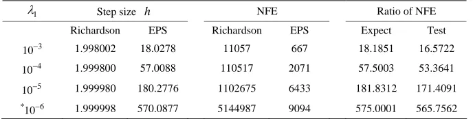
The Richardson iteration is entirely equivalent to the Euler method, so we re

ln 2 / ln 1S S . place Richardson parameter  by step size h in Table 1.

From Table 1 we can see that the ratio of NFE for theoretical expected values are basically consistent with the real calculation results and the higher the condition number is, the more efficient for our method EPS.

There is another thing need to mention. For 1= 10 6 

, EPS method taking h= 570.0877, is it possible for so large step size? In [1] Figure 1 and Figure 2 give the a

b-solute stability region for = 0.01 and  = 0.1



 = h



. Their left end points are 134 and 14. In our present case = 1.3, = 570.0877h ,  = 0.00228, using the same method we can ft end

ity region at 585.5

get the le point of the stabil  . The Max i = 1.0,

= 1, 2

i , even though we take so large step size, hi are still located at the stability region.

merical Experiment

4. Nu

he outline of our algorithm EPS is the same as des- ations to solve are T

cribed in [1]. The differential equ

 

 

=f =G



X X X (23)

 





 

1 1

or X =D f X =D G X (24) Usually we like using (24), especially when 2f

 

X

is a diagonal dominant matrix. In this case take

we simply = 0.5



For ODE (1), it is said to have a gradient stru the chain rule, we have ([3], p. 194)

cture. By

 





2



 



2

=1 =1

d d

= = =

d d

N N

i

i i i

x

f f

f t f x t

t x t x

 _   _{ }

 

 





X



(25) From (25) we see that along any analytic solution o the ODE, the quantity

f

 





f X t decreases in Euclid norm as increases.

e take ve

or, the numerical solution ean

t

Different case happens with the present method. Be- cause in our method, w ry large step size, it will

produce large local err Xn

may go far from the analytic solution X t

 

n , so we

cannot keep the condition f X



n1



< f X

 

n , especially

at the beginning of the calculation.

In some earlier literatures, for example, ]; using [6

 

*

 

_<

n

f X  f X TOL as conve t

this rule just applies to the test problems whic

rgence criteria, bu h the _X* w

not suitable, so we take

as known already. For real problems this criterion is

 

n <

G X TOL as our stop- ping criteria.

[image:4.595.127.471.622.709.2]

Example 1. The Generalized Rosenbrock Function (GENROSE) ([7], p. 421)

Table 1. 2-Dimension test problem results



λ2=λ_N= 1.0



, = 1.3ε .

1

 Step size h NFE Ratio of NFE

Richardson EPS Richardson EPS Expect Test 3

10 1.998002 18.0278 11057 667 18.1851 16.5722 2071 5 003 .3641

1.99 80 76 1102675 6433 181. 91

57 7 5 56 2

4

10 1.999800 57.0088 110517 7.5 53 5

10 9980 1 .27 8312 171.40

* 6

10 1.999998 0.087 5144987 9094 75.0001 5.756 *Note: for 1= ic ration ca any result, so we repl

6

 

f X = 1 f0

 

X

 



0 = 100 1 1

N

i

f _ x x  _

 



X 2





i 



2 1

i x_

2

= 2

i

  

0 = 1.2,1, 1.2,1,1,1, , ,1



X 1





* _{= 1,1,1, ,1 ,}

U 

X *

U

X stands for the optimal solu- .

The Gradient function:

x

tion of unconstrained problem

 



2







1 2 1 1

1 = 400 2 1

G  x x x  

 



2





2







1

= 200 i i 400 i 2 1

G i x x  x xi1xi  xi , = 2, 3,

i ,N1

 



2



1

= 200 _{N N}

G N x x _

The Diagonal of Gradient function

 

2

1 2

1 = 1200 400 2

D x  x 

 

2

1

= 1200 _i 400 _i 202 = 2, , , 1.

D i x  x_  i 3 N

As we did in [1], we divided the calculation process into three stages and took

 

= 200

D N

= 0.5,ToL1 = 1.0,ToL2 = 

, h2= 2.5, h3= 5.0. For

ve the me results:

3 5

10 , ToL3 = 10 = 100,1000,100

N

; h1= 1.0

00, we ha sa

0

= 228, = 1

NFE f  f

12

0= 0.1755 10 ,

f   _{G = 0.8771 10} 5

* 7

= 0.1174 10 .

i xi



 

1 Max

i N

x  

For large scale problem ([8], pp. 1 15) proposed a sub-space trust region method STIR. For exam le 1 the method gave two results, one was STIR with ex New- ton steps, another was STIR with inexact Newton steps. The number of iterations were 25, 21 respectively. These re

4-p act

sults showed that STIR need to solve 25 or 21 large scale linear equations [8]. Compare with our method EPS, we just need 228 times gradient function evaluation, and no linear equations were needed to solve.

It is well known that ordinary Newton method is very sensitive for the initial value. For this example



N=



100,1000,10000 all the G



X

 

0



= 0.1054 10 . 4 Or- dinary Newton method to be converged needs 375 itera- tions and get the G x(*) = 0.7389 10 6.

In order to improve the initial value, we use EPS me- thod making G X

 

 < 1 (after 33 function evalua ,

wton m nitial

value

tions) then turns to Ne ethod. For the present i

X to get the convergent result needs 229 Newton iterations. If we further improve the initial value, making

 

< 0.5

G X (after 128 function evaluations) only two

ewton steps we get

N can G X

 

* = 0.3878 10 8 19

0 = 0



.2996 10

f 

Exam The C unction (CHAIN-

OOD , p. 42 . ple 2. ) ([7]

hained 3)

Woof f W

 

= 1 0

 

f X  f X

 



2







2



2



2

0 = 100 i 1 i 1 i 90 i 3 i 2

i J

f x_ x x x_ x_



 _{    }





X





2





2





2

2 1 3 1 3

1 x_i 10 x_i x_i 2 0.1 x_i x_i ,

       _

Where N is a multiple of 4 and J = 1, 3,



5,,N3



. The Gradient function:

 



2







1 2 1 1

1 = 400 2 1

G  x x x  x

 



2







2 1 2 4

2 = 200 20 2

G x x  x x   0.2



x2x4



 



2







1

= 760 _{i i i} 4 1 _i

G i  x x_ x  x







2







1 1

1 = 380 i i 20 i i 2 G i x x  x x1



xi1 xi1



0.2



xi1 xi3



0.2    20



x_i1x_i32



,

= 3, 5, ,

i  N3







2



1

N N N

G N1 = 360 x  x x 1 2 1



xN1



 



2







1 2

= 180 _{N N} 20 _{N N} 2

G N x x _  x _ x 



2



0.2 x_N x_N

 

The diagonal of Gradient function

 

2

1 2

1 = 1200 400 2

D x  x 

 

2 = 220.2

D

 

2

1

= 2280 _i 760 _i 4

D i x  x_ 



1 = 420.4,



= 3, 5, , 3

D i i  N





2

1

1 = 1080 _N 360 _N 2

D N x _  x 

 

= 200.2

D N

As ([7], p. 423) did, for N = 8, X

  

0 =   3, 1, 3,

oblem ave the solu-



1, 2, 0, 2, 0

  

tion

the unconstrained pr h



,1,1,1,1,1



.

thod, take 

*

= 1,1,1

U

X

Use EPS me = 0.5,ToL1 = 1,ToL2 = 10 ,3 5

3 = 10 ,

ToL  h

evaluations

1= 5,

we get

2 0, 3= 15

h = 1 h ; after 572 function

5 ( ) = 0.3395 10 ,

G X   f₀=

12 0.5253 10  .

*

U

Despite we get the approximate solution

X , but for s thod does no

uch t sh

a small dimension ow the superiority expect t

problem EPS m he simp

e- licity. But we are interested in large scale problems.

For unconstrained (ChainWood) problem, , with three different start p

=

N

oints

100, 1000, 10000

 

0

(the original) 1)X

  

0 =     3, 1, 3, 1,

Take 3_{,ToL3 = 10 ,}5

1=

h 5.



2, 0,, 2, 0

= 0.5,ToL1 = 1.0, ToL2 = 10 

1 0

h , after 811 function eva- 10000 , we get same appro-f the minimal value oappro-f appro-fu

5.0, h2= 10.0, 3=

ns, for N= 100,1000,

nction f = 1 f0=

luatio

ximation o 

1 13.808 = 14.808 .



0 =    3, 1, 3, 1, 0, 0,, 0, 0 X

The parameters are the same as (1), for N = 100, after 857 function evaluations, we have f f

2)

  

0

= 1 =

10

10.18824 10  . For N= 1000,10000 after 856 f we get the same result f = 1 f0=

un-ction evaluations, 

10 9438 10  .

  

0 = 0, 1, 0, 1, 0, 0,  , 0, 0



,

1 0.1 X

3) X

 

0 is the

me

this sa

arameters are as [8].

The p

= .0,= 0.5.For N = 100,

after 628 fun e have f = 1 f0=

3

1 = 5.0, 2 = 10 , 3 =

ToL ToL  ToL

3

,h = 15

aluations, w 5

1 2

10 , h 2.0,h = 10.0

ction ev 

1 3.5743 = 4.5743 , it is exactly consistent with STIR. wh

However, SBMIM co ged to 46.713. For

ich STIR wanted to compare with,

= 1000

N , 10 , [8] did not

nver 000

give t erge. Ou

ons con

n and Y. H. Han, “Solving

tions by a New ODE Numerical Integration

3027

] P. Deuflhard, “Newton Methods for Nonlinear Problems ce and Adaptive Algorithms,” Springer- , 2004.

1996.

a

he results because SBMIM did not conv r method EPS, after 652, 659 function evaluati - verged to the same result 4.5743.

7. References

[1] T. M. Ha Large Scale

Nonlin-ear Equa

Bou

Method,” Applied Mathematics, Vol. 1, No. 3, 2010, pp. 222-229. doi: 10.4236/am.2010.1

[2

Affine Invarian Verlag, Berlin

[3] D. J. Higham, “Trust Region Algorithms and Timestep Selection,” SIAM Journal on Numerical Analysis, Vol. 37, No. 1, 1999, pp. 194-210.

doi:10.1137/S0036142998335972

[4] D. M. Young, “Convergence Properties of the Symmetric and Unsymmetric Successive Overrelaxation Methods and Related Methods,” Mathematics of Computation, Vol. 24, No. 112, 1970, pp. 793-807.

doi:10.1090/S0025-5718-1970-0281331-4

[5] Y. Saad, “Iterative Methods for Sparse Linear Systems,” PWS Publishing Company, Boston,

[6] A. Miele and J. W. Cantrell, “Study on a Memory Gradi-ent Method for the Minimization of Functions,” Journal of Optimization Theory and Applications, Vol. 3, No. 6, 1969, pp. 459-470. doi:10.1007/BF00929359

[7] A. R. Conn, N. I. M. Gould and P. L. Toint, “Testing Class of Methods for Solving Minimization Problems with Simple Bounds on the Variables,” Mathematics of Computation, Vol. 50, No. 182, 1988, pp. 399-430. doi:10.1090/S0025-5718-1988-0929544-3