Design and Power Flow Analysis of Electrical System Using Electrical Transient and Program Software

ISSN Online: 1947-3818 ISSN Print: 1949-243X

DOI: 10.4236/epe.2019.114011 Apr. 24, 2019 186 Energy and Power Engineering

Design and Power Flow Analysis of Electrical

System Using Electrical Transient and Program

Software

Raheel Muzzammel

, Ibrahim Khail, Muhammad Huzaifa Tariq,

Abubakar Muhammad Asghar, Ali Hassan

Department of Electrical Engineering, University of Lahore, Lahore, Pakistan

Abstract

Power flow analysis is a numerical way of study of behavior of flow of electric power in an interconnected system. In order to meet the growing demands of electrical energy in an optimum way, there is a need to upgrade existing sys-tems or to install new syssys-tems. Therefore, planning of new installations and determination of best operating conditions of existing systems need power flow analysis. In this way, cost/benefit ratio for both suppliers and customers is maintained. This research involves the design and power flow analysis of IEEE-14 bus system. Newton Raphson method is applied for better efficiency and reduced computational time. Simulation analysis is conducted in ETAP software because of its excessive used in real life systems.

Keywords

Power Flow Analysis, IEEE-14 Bus System, Newton Raphson Method, ETAP Software

1. Introduction

Behavior of flow of electric power in an interconnected system is studied nu-merically by power flow analysis. Single line diagram and per unit system are the

fundamental components of this analysis. Voltage (V), voltage angles (δ), active

power (P) and reactive power (Q) are the variables involved in this study. Active

power and voltage are known at supply side and reactive power and voltage an-gles are determined through numerical analysis of power flow. Active power and reactive power are known at consumer side and voltage and voltage angles are

evaluated through power flow analysis [1][2][3].

How to cite this paper: Muzzammel, R., Khail, I., Tariq, M.H., Asghar, A.M. and Hassan, A. (2019) Design and Power Flow Analysis of Electrical System Using Electrical Transient and Program Software. Energy and Power Engineering, 11, 186-199. https://doi.org/10.4236/epe.2019.114011

Received: March 17, 2019 Accepted: April 21, 2019 Published: April 24, 2019

Copyright © 2019 by author(s) and Scientific Research Publishing Inc. This work is licensed under the Creative Commons Attribution International License (CC BY 4.0).

DOI: 10.4236/epe.2019.114011 187 Energy and Power Engineering

There is a requirement to improve current power system or to add new sys-tems to existing syssys-tems for meeting energy demands. Therefore, power flow analysis is an essential study for future expansion of power system and for find-ing the ideal operatfind-ing conditions of existfind-ing electric power systems. Moreover, economic dispatch, unit commitment, contingency analysis, transient and steady

state analysis and short circuit analysis require power flow analysis [2][3].

In power flow analysis, there are three types of buses i.e., swing bus, generator

bus and load bus. Swing bus and generator bus are source buses. For swing bus,

V and δ are known and P and Q are unknown values. The source bus with larger

size of generator is normally taken as swing bus. For generator bus (PV bus), P

and V are known values and Q and δ are unknown. For load bus (PQ bus), P

and Q are known and V and δ are unknown values. The unknown parameters of

buses (i.e., P and Q for swing bus, Q and δ for generator bus and V and δ for

load bus) are determined from known values of buses (i.e., V and δ for swing

bus, P and V for generator bus and P and Q for load bus) and impedance

be-tween these buses (Zij) using power flow calculations. After performing power

flow analysis, all the four parameters (V, δ, P and Q) are available for swing bus,

generator bus and load bus. The other electrical parameters such as current, power factor, apparent power for the whole electrical system can be determined

from these four parameters (V, δ, P and Q) and impedance between the buses

(Zij) [2][3].

Commercial power systems are complicated. It is not possible to analyze power flow through hand calculations. Physical models of power systems were analyzed through network analyzers in laboratories between 1929 and early 1960. Afterwards, invention of digital computers replaced the analog methods

with numerical methods [1]-[7].

Initially, linear methods were proposed to analyze power flow analysis.

Among these, Cramer’s method, Gauss elimination and LU factorization are

notable. However, these methods cannot handle complex, nonlinear and big

power systems. Therefore, iterative techniques i.e., Gauss Seidel method,

New-ton Raphson method are developed to solve complex power systems [4][5][6]

[7][8].

In this research paper, Newton Raphson method is implemented because of its accuracy and reduced computational time due to less iteration as compared to

Gauss Seidel method. Iterative methods are techniques for solving the n

equa-tions of the linear system Ax b= one at a time in sequence, and use previously

ac-DOI: 10.4236/epe.2019.114011 188 Energy and Power Engineering

quires more memory space then Gauss Seidel method. Time required for per iteration in Newton Raphson method is larger than Gauss Seidel method but the overall time for iterative process is less because of less number of iterations for

convergence [1][2][3][4][7][8][9].

ETAP software is used for simulation because of its extension of real time in-telligent power management systems for monitoring, controlling, automating and optimizing power systems. It is a high impact software used for power flow analysis is generation, transmission and distribution systems of electric power

engineering [10][11][12][13].

This research paper consists of following sections: Section II covers the ma-thematical background and proposed flow chart for Newton Raphson method. Section III contains the details of IEEE-14 bus system as a test model for depict-ing accuracy of power flow analysis method. Simulation analysis in tabular form is presented in Section IV. Section V concludes the research.

2. Newton Raphson Method

Newton Raphson method is named after Isaac Newton and Joseph Raphson. Successively better approximations for the roots of a real-valued function are determined from this method. Newton-Raphson load flow analysis is based on Newton Raphson method for evaluation of a system of nonlinear equations. It is an iterative method which approximates a set of non-linear simultaneous equa-tions is approximated to a set of linear simultaneous equaequa-tions using Taylor’s

se-ries expansion by this iterative method [2][3].

Referring to Figure 1, polar form of power flow equations are formulated for

n bus system in terms of bus admittance matrix Y as

1

n i j ij j

I =

∑

(

)

1|

n

i j ij j ij j

I =

∑

where i and j represent _ith _{and j}th _{bus respectively. The current in terms of}

the active and the reactive power at bus i is:

i i

i i

P JQ I

V −

= ₍₃₎

Using Equation (3) into Equation (2) gives:

1

n i

i i i i j ij ij j

P jQ− =V < −

δ

∑

θ

δ

1

n

i i i i j ij ij j i

P jQ− =

∑

θ

δ

δ

Real and imaginary parts are separated as:

(

)

1 cos

n

i i i j ij ij j i

P =

∑

θ

δ

δ

(

)

1 sin

n

i i i j ij ij j i

Q = −

∑

θ

δ

δ

DOI: 10.4236/epe.2019.114011 189 Energy and Power Engineering

Figure 1. Typical power system bus bar model.

2 2 2 2

2 2 2 2

2 2

2 2 2

2

2 2 2 2

2 2 2 2 n n n n n n n n n n n n n n n n

P P P P

V V _P

P P P P

V V P

V

Q Q Q Q

V V

V

Q Q Q Q

V V

δ δ δ

δ δ δ

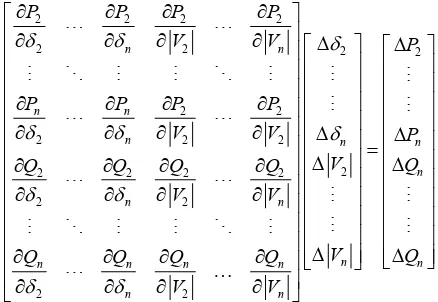
δ δ δ δ ∂ ∂ ∂ ∂   _{∂ ∂ ∂ ∂}  _{∆ ∆}    _{ }  _{ }     ∂ ∂ ∂ ∂  _{ } _{∂ ∂ ∂ ∂} _{∆  ∆}  _{ }= ∆ ∆ ∂ ∂ ∂ ∂  _{ } _{∂ ∂ ∂ ∂} _{ }      _{ }  _{ ∆ } ∂ ∂ ∂ ∂ _{ }  _…  _{∂ ∂ ∂ ∂}                             n n Q Q                       ∆       (8)

Linearized relationship is obtained by this Jacobian matrix between small

changes in voltage angles ∆δi and voltage magnitude ∆Vi with the small

changes in real and reactive power ∆Pi and ∆Qi. (8) can be modified as:

1 2 3 4 J J P V J J Q δ ∆ ∆      =_{  } _∆  _∆

      (9)

The diagonal and the off diagonal elements of J1 are:

(

)

sin

i

i j ij ij j i j i

i

P _{V V Y θ δ δ}

δ ≠

∂

= + −

∂

∑

(

)

sin

i

i j ij ij j i

j

P _{V V Y θ δ δ} δ

∂ _{= − + −}

∂ (11)

where j i≠ .

(

)

1 sin

n i

i j ij ij j i j

j

Q _{VV Y θ δ δ}

δ =

∂ _{= + −}

∂

∑

Similarly, diagonal and off diagonal elements of J2, J3, J4 are:

(

)

2 cos cos

i

i ii ii j i j ij ij j i

i

P _{V Y V Y}

V θ ≠ θ δ δ

∂

= + + −

∂

∑

(

)

cos

i

i ij ij j i

j

P _{V Y}

V θ δ δ

∂

= + −

∂ (13)

DOI: 10.4236/epe.2019.114011 190 Energy and Power Engineering

(

)

cos

i

i j ij ij j i j i

i

Q _{V V Y θ δ δ}

δ ≠

∂

= + −

∂

∑

(

)

cos

i

i j ij ij j i

j

P _{V V Y θ δ δ} δ

∂

= − + −

∂ (15)

(

)

2 sin sin

| |i i ij ii j i i ij ij j i

i

Q _{V Y V Y}

V θ ≠ θ δ δ

∂

= − + + −

∂

∑

(

)

sin

i

i ij ij j i

j

Q _{V Y}

V θ δ δ

∂

= − + −

∂ (17)

The terms ∆Pi and ∆Qi in Equation (8) are the differences between the

scheduled and calculated values of power called power residuals given as: sch

i i i

P P P

∆ = − (18)

sch

i i i

Q Q Q

∆ = − ₍₁₉₎

Using Equation (8), Equation (18) and Equation (19), ∆δi and ∆Vi are

calculated to complete the particular iteration. The new values calculated as

shown below are used for the next iteration (k + 1)

1

k k k

i i i

δ + ₌δ _{− ∆}δ ₍₂₀₎

1

k k k

i i i

V + ₌V _{− ∆}V ₍₂₁₎

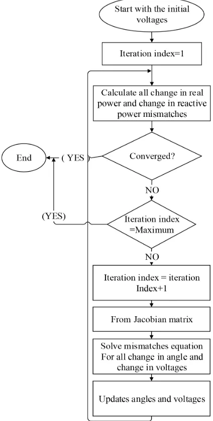
Flow chart of Newton Raphson method is given in Figure 2. Test system i.e.,

IEEE 14 bus system is analyzed in Figure 3.

3. Test System—IEEE 14 BUS System

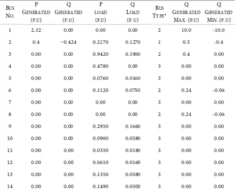
IEEE 14 bus system is used to validate the performance of Newton Raphson

method. Table 1 and Table 2 provide the details of buses data and branches data

for power system. In Table 1, *Bus Type (1) represents swing bus, (2) represents

generator bus (PV bus) and (3) represents load bus (PQ bus).

4. Simulation Analysis

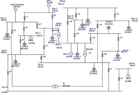
ETAP software is used for simulation analysis and simulation circuit is given in

Figure 4. Power flow analysis for IEEE-14 bus system is carried out by Newton

Raphson method. Table 3 provides the results of power flow analysis on

branches of electric power system.

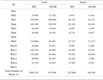
Table 4 gives the detail of load and losses in electric power system after power flow analysis via Newton Raphson method. IEEE-14 bus system after power flow

analysis is given in Figure 5.

Power flow analysis results in generation of alerts at generators. The alerts

contain the conditions of operation of generator as shown in Table 5.

Condi-tions of operation of generators are overload, overexcited, under excited and normal. After taking into consideration the capability curve and load values, the generation values are readjusted to bring operation of generators under normal

DOI: 10.4236/epe.2019.114011 191 Energy and Power Engineering

Figure 2. Flow chart of Newton Raphson method.

DOI: 10.4236/epe.2019.114011 192 Energy and Power Engineering

Table 1. This table shows the bus data of IEEE-14 bus system.

BUS

NO.

P

GENERATED

(P.U)

Q

GENERATED

(P.U)

P

LOAD

(P.U)

Q LOAD

(P.U)

BUS

TYPE*

Q

GENERATED

MAX.(P.U) Q

GENERATED

MIN.(P.U) 1 2.32 0.00 0.00 0.00 2 10.0 -10.0 2 0.4 −0.424 0.2170 0.1270 1 0.5 -0.4 3 0.00 0.00 0.9420 0.1900 2 0.4 0.00 4 0.00 0.00 0.4780 0.00 3 0.00 0.00 5 0.00 0.00 0.0760 0.0160 3 0.00 0.00 6 0.00 0.00 0.1120 0.0750 2 0.24 -0.06 7 0.00 0.00 0.00 0.00 3 0.00 0.00 8 0.00 0.00 0.00 0.00 2 0.24 -0.06 9 0.00 0.00 0.2950 0.1660 3 0.00 0.00 10 0.00 0.00 0.0900 0.0580 3 0.00 0.00 11 0.00 0.00 0.0350 0.0180 3 0.00 0.00 12 0.00 0.00 0.0610 0.0160 3 0.00 0.00 13 0.00 0.00 0.1350 0.0580 3 0.00 0.00 14 0.00 0.00 0.1490 0.0500 3 0.00 0.00

Table 2. This table shows the branch data of IEEE-14 bus system.

From Bus To Bus Resistance (p.u.) Reactance (p.u) Line charging (p.u.) 1 2 0.01938 0.05917 0.0528 1 5 0.05403 0.22304 0.0492 2 3 0.04699 0.19797 0.0438 2 4 0.05811 0.17632 0.0374 2 5 0.05695 0.17388 0.034 3 4 0.06701 0.17103 0.0346 4 5 0.01335 0.04211 0.0128

4 7 0.00 0.20912 0.00

4 9 0.00 0.55618 0.00

5 6 0.00 0.25202 0.00

6 11 0.09498 0.1989 0.00 6 12 0.12291 0.25581 0.00 6 13 0.06615 0.13027 0.00

7 8 0.00 0.17615 0.00

7 9 0.00 0.11001 0.00

DOI: 10.4236/epe.2019.114011 193 Energy and Power Engineering

Table 3. This table provides the result of power flow analysis of on branches of IEEE-14

bus system.

ID Type From Bus To Bus R X Z T1 2W XFMR Bus5 Bus6 554.70 832.05 1000 T2 2W XFMR Bus9 Bus6 554.70 832.05 1000. T5 2W XFMR Bus9 Bus4 69.43 3124.23 3125 Z1 Impedance Bus1 Bus2 0.00 0.01 0.01 Z2 Impedance Bus1 Bus5 0.01 0.04 0.04 Z3 Impedance Bus3 Bus4 0.01 0.03 0.03 Z4 Impedance Bus2 Bus3 0.01 0.04 0.04 Z5 Impedance Bus2 Bus4 0.01 0.03 0.04 Z6 Impedance Bus5 Bus4 0.00 0.01 0.01 Z7 Impedance Bus9 Bus15 0.02 0.02 Z8 Impedance Bus4 Bus15 0.04 0.04 Z9 Impedance Bus8 Bus15 0.03 0.03 Z10 Impedance Bus10 Bus9 0.01 0.02 0.02 Z11 Impedance Bus11 Bus10 0.02 0.04 0.04 Z12 Impedance Bus11 Bus6 0.02 0.04 0.04 Z13 Impedance Bus12 Bus6 0.02 0.05 0.05 Z14 Impedance Bus13 Bus12 0.04 0.04 0.06 Z15 Impedance Bus13 Bus14 0.03 0.07 0.07 Z16 Impedance Bus14 Bus9 0.02 0.05 0.06 Z17 Impedance Bus5 Bus2 0.01 0.03 0.03 Z18 Impedance Bus4 Bus9 0.11 0.11 Z19 Impedance Bus13 Bus6 0.13 0.02 0.13

Table 4. This table shows the result of load and losses after load flow analysis at 230 kv

and at 100 percent magnitude.

ID Load Losses

MW MVAR MW MVAR

Bus1 - - - -

Bus2 27.880 17.278 6.970 4.320 Bus3 336.600 208.606 84.150 52.151 Bus4 169.320 104.935 42.330 26.234 Bus5 26.520 16.436 6.630 4.109 Bus6 42.840 26.550 10.710 6.637

Bus8 - - - -

Bus9 110.840 68.692 27.710 17.173 Bus10 34.000 21.071 8.500 5.268 Bus11 104.720 64.900 26.180 16.225 Bus12 135.320 83.864 33.830 20.966 Bus13 48.960 30.343 12.240 7.586 Bus14 53.720 33.293 13.430 8.323

Bus15 - - - -

Total Number of

DOI: 10.4236/epe.2019.114011 194 Energy and Power Engineering

Table 5. This table gives the condition of three phase generators after power flow analysis

via Newton Raphson method.

Device ID Condition Rating/limit Operating %Operating Gen1 Overload 60 MW 60 100 Gen1 Over Excited 37.5 Mvar 37.185 100 Gen2 Overload 25 MW 25 100 Gen2 Under Excited 0 0 - Gen3 Overload 25 MW 25 100

Gen3 Under Excited 0 -

Gen4 Overload 60 MW 60 100

Gen4 Under Excited 0 -

Swing Gen Overload 615 MW 1193.143 194

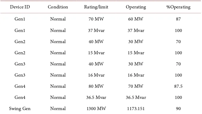
Table 6. This table gives the values of generation under normal operating conditions

of generators.

Device ID Condition Rating/limit Operating %Operating Gen1 Normal 70 MW 60 MW 87 Gen1 Normal 37 Mvar 37 Mvar 100 Gen2 Normal 40 MW 30 MW 70 Gen2 Normal 15 Mvar 15 Mvar 100 Gen3 Normal 40 MW 30 MW 70 Gen3 Normal 16 Mvar 16 Mvar 100 Gen4 Normal 80 MW 70 MW 87.5 Gen4 Normal 36.5 Mvar 36.5 Mvar 100 Swing Gen Normal 1300 MW 1173.151 90

ETAP report is generated and is given in Table 7 to depict the generation and

load in electric power system test model.

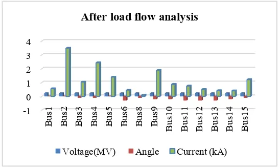
Voltage and current of test system are measured before and after load flow

analysis to depict the state of the system and are shown in Figure 6 and Figure

7. Change in the values of voltage and angles are observed. It is the requirement

of power system to have good voltage regulation for ensuring acceptable power factor value.

5. Conclusion

DOI: 10.4236/epe.2019.114011 195 Energy and Power Engineering

Figure 4. This figure shows the simulation circuit of IEEE-14 bus system on ETAP software.

DOI: 10.4236/epe.2019.114011 196 Energy and Power Engineering

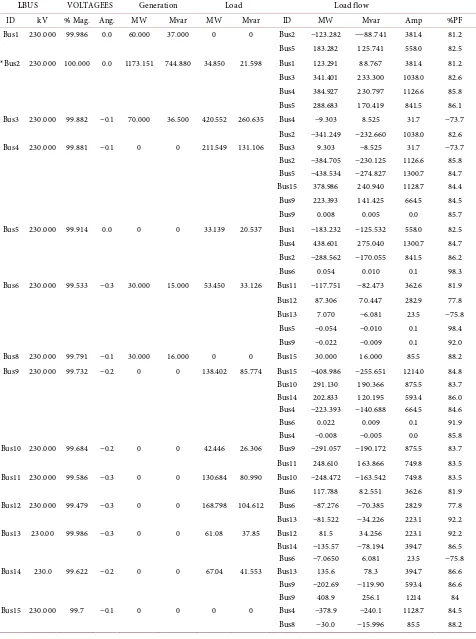
Table 7. This table shows the load flow ETAP software report via Newton Rahson method.

LBUS VOLTAGEES Generation Load Load flow

ID kV % Mag. Ang. MW Mvar MW Mvar ID MW Mvar Amp %PF Bus1 230.000 99.986 0.0 60.000 37.000 0 0 Bus2 −123.282 −−88.741 381.4 81.2 Bus5 183.282 125.741 558.0 82.5 *Bus2 230.000 100.000 0.0 1173.151 744.880 34.850 21.598 Bus1 123.291 88.767 381.4 81.2 Bus3 341.401 233.300 1038.0 82.6 Bus4 384.927 230.797 1126.6 85.8 Bus5 288.683 170.419 841.5 86.1 Bus3 230.000 99.882 −0.1 70.000 36.500 420.552 260.635 Bus4 −9.303 8.525 31.7 −73.7

Bus2 −341.249 −232.660 1038.0 82.6 Bus4 230.000 99.881 −0.1 0 0 211.549 131.106 Bus3 9.303 −8.525 31.7 −73.7

Bus2 −384.705 −230.125 1126.6 85.8 Bus5 −438.534 −274.827 1300.7 84.7 Bus15 378.986 240.940 1128.7 84.4 Bus9 223.393 141.425 664.5 84.5 Bus9 0.008 0.005 0.0 85.7 Bus5 230.000 99.914 0.0 0 0 33.139 20.537 Bus1 −183.232 −125.532 558.0 82.5 Bus4 438.601 275.040 1300.7 84.7 Bus2 −288.562 −170.055 841.5 86.2 Bus6 0.054 0.010 0.1 98.3 Bus6 230.000 99.533 −0.3 30.000 15.000 53.450 33.126 Bus11 −117.751 −82.473 362.6 81.9 Bus12 87.306 70.447 282.9 77.8 Bus13 7.070 −6.081 23.5 −75.8

Bus5 −0.054 −0.010 0.1 98.4 Bus9 −0.022 −0.009 0.1 92.0 Bus8 230.000 99.791 −0.1 30.000 16.000 0 0 Bus15 30.000 16.000 85.5 88.2 Bus9 230.000 99.732 −0.2 0 0 138.402 85.774 Bus15 −408.986 −255.651 1214.0 84.8 Bus10 291.130 190.366 875.5 83.7 Bus14 202.833 120.195 593.4 86.0 Bus4 −223.393 −140.688 664.5 84.6 Bus6 0.022 0.009 0.1 91.9 Bus4 −0.008 −0.005 0.0 85.8 Bus10 230.000 99.684 −0.2 0 0 42.446 26.306 Bus9 −291.057 −190.172 875.5 83.7 Bus11 248.610 163.866 749.8 83.5 Bus11 230.000 99.586 −0.3 0 0 130.684 80.990 Bus10 −248.472 −163.542 749.8 83.5 Bus6 117.788 82.551 362.6 81.9 Bus12 230.000 99.479 −0.3 0 0 168.798 104.612 Bus6 −87.276 −70.385 282.9 77.8 Bus13 −81.522 −34.226 223.1 92.2 Bus13 230.00 99.986 −0.3 0 0 61.08 37.85 Bus12 81.5 34.256 223.1 92.2 Bus14 −135.57 −78.194 394.7 86.5 Bus6 −7.0650 6.081 23.5 −75.8 Bus14 230.0 99.622 −0.2 0 0 67.04 41.553 Bus13 135.6 78.3 394.7 86.6

Bus9 −202.69 −119.90 593.4 86.6 Bus9 408.9 256.1 1214 84 Bus15 230.000 99.7 −0.1 0 0 0 0 Bus4 −378.9 −240.1 1128.7 84.5

DOI: 10.4236/epe.2019.114011 197 Energy and Power Engineering

Figure 6. Graphical representation of voltage and current of IEEE-14 bus

system before power flow analysis.

Figure 7. Graphical representation of voltage and current of IEEE-14 bus

system after power flow analysis.

taking into consideration capability curve and load values to bring operation of generators under normal conditions. It is found that power flow analysis is comprehensively conducted through Newton Raphson method via ETAP soft-ware. This research depicts the importance of implementing Newton Raphson and using ETAP software at industrial and commercial levels. With a little change in voltage values at buses of power system, generators are brought to normal operating conditions. Power factor is not much compromised. Load is meeting in economic operating conditions. Weak branches are identified. Ca-pacitor banks and static volt Ampere reactive compensator (SVC) would be the ultimate solution to make them strong. This load flow study would lead to the installation of flexible alternating current transmission system (FACTS) devices for reactive power compensation. This research led to the development of opti-mization algorithms for finding the location of FACTS devices. Transient and economic dispatch for circuit breaker placements and economics of generations will be the future work of this power flow analysis.

0 1 2 3 4 Bu s1 Bu s2 Bu s3 Bu s4 Bu s5 Bu s6 Bu s8 Bu s9 B us 10 B us 11 B us 12 B us 13 B us 14 B us 15

Before load flow analysis

Voltage(MV) Angle Current(KA)

-1 0 1 2 3 4 Bu s1 Bu s2 Bu s3 Bu s4 Bu s5 Bu s6 Bu s8 Bu s9 Bus 10 Bus 11 Bus 12 Bus 13 Bus 14 Bus 15

After load flow analysis

DOI: 10.4236/epe.2019.114011 198 Energy and Power Engineering

Conflicts of Interest

The authors declare no conflicts of interest regarding the publication of this paper.

References

[1] Muzzammel, R., Ahsan, M. and Ahmad, W. (2015) Non-Linear Analytic

Ap-proaches of Power Flow Analysis and Voltage Profile Improvement. 2015 Power

Generation System and Renewable Energy Technologies (PGSRET), Islamabad,

June 2015, 1-7.

[2] Saadat, H. (1999) Power System Analysis. Mc Graw-hill, Inc., 2 Pennsylvania Plaza

New York City.

[3] Stevenson, W.D. (1982) Elements of Paver System Analysis. McGraw-Hill, 2

Penn-sylvania Plaza New York City.

[4] Athay, T. (1983) An Overview of Power Flow Analysis. 1983 American Control

Conference, San Francisco, CA, USA,22-24 June 1983, 404-410.

https://doi.org/10.23919/ACC.1983.4788145

[5] Mešanović, A., Münz, U. and Ebenbauer, C. (2018) Robust Optimal Power Flow for

Mixed AC/DC Transmission Systems with Volatile Renewables. IEEE Transactions

on Power Systems, 33, 5171-5182. https://doi.org/10.1109/TPWRS.2018.2804358

[6] Levron, Y., Guerrero, J.M. and Beck, Y. (2013) Optimal Power Flow in Microgrids

with Energy Storage. IEEE Transactions on Power Systems, 28, 3226-3234.

https://doi.org/10.1109/TPWRS.2013.2245925

[7] Stott, B. (1974) Review of Load-Flow Calculation Methods. Proceedings of the

IEEE, 62, 916-929. https://doi.org/10.1109/PROC.1974.9544

[8] Fikri, M., Cheddadi, B., Sabri, O., Haidi, T., Abdelaziz, B. and Majdoub, M. (2018)

Power Flow Analysis by Numerical Techniques and Artificial Neural Networks.

2018 Renewable Energies, Power Systems & Green Inclusive Economy (REPS-GIE),

Casablanca, 23-24 April 2018, 1-5. https://doi.org/10.1109/REPSGIE.2018.8488870

[9] Montoya, O.D., Garrido, V.M., Gil-González, W. and Grisales-Noreña, L. (2019)

Power Flow Analysis in DC Grids: Two Alternative Numerical Methods. IEEE

Transactions on Circuits and Systems II: Express Briefs, 1-1.

https://doi.org/10.1109/TCSII.2019.2891640

[10] Asrari, A. and Ramos, B. (2018) Power System Protection Upgrade at Anclote Plant

a Case Study in Florida State. 2018 IEEE Texas Power and Energy Conference

(TPEC), College Station, TX, 8-9 February 2018, 1-6.

https://doi.org/10.1109/TPEC.2018.8312091

[11] Chandraratne, C., Woo, W.L., Logenthiran, T. and Naayagi, R.T. (2018) Adaptive

Overcurrent Protection for Power Systems with Distributed Generators. 2018 8th

International Conference on Power and Energy Systems (ICPES), Colombo, Sri

Lanka, 21-22 December 2018, 98-103.

https://doi.org/10.1109/ICPESYS.2018.8626908

[12] Soni, C.J., Gandhi, P.R. and Takalkar, S.M. (2015) Design and Analysis of 11 KV

Distribution System Using ETAP Software. 2015 International Conference on

Computation of Power, Energy, Information and Communication (ICCPEIC),

Chennai, Chennai, 22-23 April 2015, 0451-0456.

DOI: 10.4236/epe.2019.114011 199 Energy and Power Engineering

[13] Alinejad-Beromi, Y., Sedighizadeh, M., Bayat, M.R. and Khodayar, M.E. (2007)

Us-ing Genetic Alghoritm for Distributed Generation Allocation to Reduce Losses and

Improve Voltage Profile. 2007 42nd International Universities Power Engineering

Conference, Brighton, 4-6 September 2007, 954-959.