Reactive Power and FACTS Cost Models’ Impact on Nodal Pricing in Hybrid Electricity Markets

Reactive Power and FACTS Cost Models’ Impact

on Nodal Pricing in Hybrid Electricity Markets

Ashwani Kumar

Department of Electrical Engineering, National Institute of Technology, Kurukshetra, India. Email: ashwa_ks@yahoo.co.in

Received December 31, 2010; revised May 23, 2011; accepted May 30, 2011.

ABSTRACT

In a competitive environment reactive power management is an essential service provided by independent system operator taking into account the voltage security and transmission losses. The system operator adopts a transparent and non-discriminatory procedure to procure the reactive power supply for optimal deployment in the system. Since genera-tors’ are the main source of reactive power generation and the cost of the reactive power should be considered for their noticeable impact on both real and reactive power marginal prices. In this paper, a method based on marginal cost theory is presented for locational marginal prices calculation for real and reactive power considering different reactive power cost models of generators’ reactive support. With the presence of FACTS controllers in the system for more flexible opera-tion, their impact on nodal prices can not be ignored for wheeling cost determination and has also to be considered taking their cost function into account. The results have been obtained for hybrid electricity market model and results have also been computed for pool model for comparison. Mixed Integer Non-linear programming (MINLP) approach has been for-mulated for solving the complex problem with MATLAB and GAMS interfacing. The proposed approach has been tested on IEEE 24-bus Reliability Test System (RTS).

Keywords:Real and Reactive Power, Nodal Price, Reactive Power Cost Model, FACTS Cost Model, Bilateral

Transactions, Hybrid Market Model

1. Introduction

In a competitive environment, the transmission system operator is responsible for proper coordination of genera-tion and transmission facilities. The reactive power ser-vice is essentially required for transmission of active power, control of voltage, and normal and secure opera-tion of a power system. Due to this reason, the reactive power support service has been identified as one of the key ancillary services in the competitive electricity mar-ket structures. Therefore, real time reactive power pricing addresses the important issue of providing information to both utility and consumers about the actual burden on the system and its better and economic operation of system. Real time reactive power price has shown to perform better than the power factor penalty scheme in terms of providing incentives to all customers to optimally man-age their reactive power consumption irrespective of their power factor [1,2]. Therefore, with the growing interest in determining the costs of ancillary services needed to maintain the quality of supply, the spot price for reactive power has also gained considerable attention

in competitive electricity markets.

Reactive Power and FACTS Cost Models’ Impact on Nodal Pricing in Hybrid Electricity Markets 231

resent the marginal costs of the node power injections [1]. The account of the reactive power production cost by introducing MVAR cost curves, which are a part of MW incremental cost curve was given in [2]. The successive LP method was applied to solve this non-linear reactive power optimization problem. Reference [7] developed reactive power pricing scheme through employing P-Q decoupled OPF to obtain SRMC of active and reactive power respectively and emphasized that the production cost of reactive power should be accounted for when pricing wheeling transactions. The authors directly in-troduced real power loss component into reactive power spot pricing derived from the Q-sub-problem with the objective of minimizing the real power loss and the in-fluence of reactive power on the voltage level appears in the pricing formulae. Authors determined the wheeling marginal cost of reactive power in [8].

Due to the growing interest in the determination of costs of supplying of ancillary services, spinning reserve, congestion alleviation cost, and security, the spot price must be decomposed to obtain the different pricing com- ponents [9-14]. Considering the most ancillary services and incorporating the constraints on power quality and environment, an advance pricing structure was recently introduced [11], which combined dynamic equations for load frequency control with static equations of con-strained OPF, however, the method is quite complex to solve. A simple approach was presented to reactive pow-er planning and combines the issue with reactive powpow-er pricing so as to recover the cost of installed capacitors using OPF approach [13]. Authors presented theory and simulation results of real time pricing of real and reactive power using a social benefit function [14]. In [15] a de-tailed discussion on reactive power service is made and it is shown that the capital costs should be included in the reactive power price. Lamont and Fu [16] introduced opportunity cost as a reactive power production cost of generator, however the computation of the cost is diffi-cult. A summary of the modifications of OPF algorithms in reactive power pricing was presented along with their features in [17]. A methodology for reactive power prices calculation with decoupled optimization was presented in [18]. Authors determined spot prices of reactive power and proposed two practical proposals for the procurement and charging of reactive and voltage control services [19]. Authors proposed a formulation of active and reactive power has been presented considering production costs of reactive power and active losses minimization in the objective function [20]. Recently, a new formulation has been considered for calculating the cost of reactive pow-er production by the use of nonlinear model that repre-sents the loss of opportunity in active power including the detailed model of the heating limits of the armature and field, and under excitation limit. Active and reactive

power marginal prices are calculated with a modified OPF that uses sequential linear program- ming technique with a modified interior point method [21].

In the present pace of power system restructuring, transmission systems are being required to provide in-creased power transfer capability and to accommodate a much wider range of possible generation patterns over a large geographic area. The demand of better utilization of existing power system and to increase power transfer capability by installing FACTS (Flexible AC Transmis-sion Systems) controllers have become imperative. In-stallation of these controllers with their optimal location can change power flow patterns, stability, security, reli-ability, and economic efficiency of the system by chang-ing wheelchang-ing cost of power due to the impact on nodal prices of both real and reactive power. Therefore, these devices cost functions should also be incorporated in an objective function for noticeable changes in nodal prices of both the real and reactive power [22,23]. Olivera, et al. presented allocation of FACTS devices and their role in the change of production cost and transmission pricing [24]. Srivastava and Verma determined the spot prices of real and reactive power maximizing social welfare func-tion and impact of SVC and TCSC on the spot prices were also studied [25]. Recently, Shrestha and Feng pre-sented simulation studies on the effects of TCSC on the spot price of real and reactive power using heuristic me-thod to determine the location of TCSC [26]. Authors presented effects of optimally located SVC and TCPAR on the real and reactive power price including the costs of FACTS controllers [27]. However, the cost of FACTS controllers has not been considered in the model for their impact on nodal prices. In a deregulated environment, the number of bilateral transactions has grown rapidly [28-31]. It is therefore essential to help the system op-erator to evaluate their impacts on the system operation and evaluating their impact on nodal prices.

In this paper, impact on nodal prices have been deter-mined considering three different reactive cost model for generators’ reactive power cost calculations for hybrid electricity markets where pool and bilateral transactions are occurring simultaneously. The impact of FACTS controllers have been incorporated taking their cost func-tions into account for evaluating their impact on nodal prices of real and reactive power. The complex problem has been solved using GAMS and MATLAB interfacing with DICOPT model in GAMS [32,33]. The comparison has been given for different reactive cost models for IEEE 24-bus reliability test system [34].

2. A Bilateral Transaction Matrix-T

traded and the trade prices are at the discretion of these parties and not a matter of ISO. These transactions are then brought to the ISO with a request that transmission facilities for the relevant amount of power be provided. If there is no violation of static and dynamic security, the ISO simply dispatches all requested transactions and charges for the service.

The bilateral concept can be generalized to the multi- node case where the seller, for example a generation company called Gencos, may inject power at several nodes and the buyer bus called Discos also draw load at several nodes. Unlike pool dispatch, there will be a transaction power balance in that the aggregate injection equals the aggregate draw off for each transaction.The bilateral contract model used in this paper is basically a subset of the full transaction matrix proposed in [28]. In its general form, the transaction matrix T as shown in (1) is a collection of all possible transactions between Gen-eration (G), Demand (D), and any other trading Entities (E) such as the marketers and the brokers.

GG GD GE DG DD DE EG ED EE

 

  

 

 

T _ (1)

In this work, all transactions have been considered between the suppliers (G) and consumers (D). It is also noted that the diagonal block matrices (GG and DD) are zero because it is assumed that there are no contracts made between two suppliers or two consumers. Neglect-ing transmission losses, the transaction matrix can be simplified as:

 

 

GD DG 

g



,

(2)

Each element of transaction matrix GD, namely GDij, represents a bilateral contract between a supplier (Pgi) of row i with a consumer (Pdj) of column j. Furthermore, the sum of row i represents the total power produced by ge-nerator i and the sum of column j represents the total power consumed at load j.

1,1 1,

2,1 2,

,1 ,

nd nd ng ng nd

GD GD

GD GD

GD GD

 

 

  

 

 

GD

  

(3)

where:

ng = number of generators, and nd = number of loads. In general, the conventional load flow variables, gene- ration (Pg) and load (Pd) vectors, are now expanded into two dimensional transaction matrix GD as given in (4).

0 0

T d

g d

     



     

 

   

P GD u

P GD u (4)

Vector ug and ud are column vectors of ones with the dimensions of ng and nd respectively. There are some intrinsic properties associated with this transaction ma-trix GD [25]. These are column rule, row rule, range rule, and flow rule. These properties have been explained in [25]. Each contract has to range from zero to a maximum allowable value, GDijmax. This maximum value is bounded by the value of corresponding PGimax or PDj whichever is smaller. The range rule satisfies:



max max

0GDijGDij min PGi PDj (5) It is also possible for some contracts to be firm so that is equal to [30]. According to flow rule the line flows of the network using AC model can be expressed as follows:

0

ij

GD max

ij

GD





line G D

P ACDF P P (6)

The matrix ACDF is the distribution factors matrix [35]. If the representations of the Pg and Pd are substi-tuted by using the definition of GD as given in (4), the line flows can be expressed in an alternative as follows:

1

1

T line

    

 _  _{ }

   



P ACDF GD GD 



(7)



max max

, ,

min ,

sb GB sb D

GD  P P_{B bb} (8) Bilateral transactions for IEEE-24 bus system have been considered and are given in Table 1. These transac-tions are taken as additional transactransac-tions over and above the already committed pool transactions taken in a sys-tem.

3. Reactive Power Cost Model for

Generators’ Reactive Power

The cost of reactive power produced by a generator is essentially composed of two components: fixed costs or investment costs and variable costs. Variable cost in turn consists of operating costs (including fuel and mainte-nance cost) and the opportunity cost which depend on the reduction in its active power generation. Three methods have been considered to evaluate the cost of reactive power of generators.

3.1. Method-1: Triangular Approach [22]

This method of reactive power cost calculation is essen-tially based on the formulation for active power cost, in which the active power is replaced by reactive power using the triangular relationship.

 

Reactive Power and FACTS Cost Models’ Impact on Nodal Pricing in Hybrid Electricity Markets 233

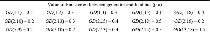
Table 1. Values of transactions between generators’ and loads.

Value of transaction between generator and load bus (p.u)

GD(1,1) = 0.5 GD(1,2) = 0.3 GD(1,3) = 0.3 GD(1,15) = 0.1 GD(1,18) = 0.4

GD(2,10) = 0.2 GD(2,13) = 0.3 GD(2,15) = 0.4 GD(2,18) = 0.5 GD(2,19) = 0.2

GD(7,9) = 0.2 GD(7,10) = 0.2 GD(7,13) = 0.4 GD(7,15) = 0.5 GD(13,18) = 1.5

tor (cos θ) and are calculated as follows from power tri-angle are:

sin 2 , sin ,

p p p

aa  bb  cc (10)

3.2. Method-2: Maximum Real Power (Pmax) Based Approach

If a generator produces (Pmax) as its maximum active power, then its cost for generating active power equals to cost (Pmax). In such a situation, no reactive power is pro-duced and therefore, S equals Pmax. Reactive power duction by a generator will reduce its capability to pro-duce active power. Hence, provision of reactive power produced by generator will result in reduction of its ac-tive power production.To generate reactive power Qiby generator i which has been operating at its nominal pow-er (Pmax), it is required to reduce its active power to Pi

such that:

2 2

max , max

i i

P  P Q  P P P_i (11)

ΔP represents the amount of active power that will be reduced as a result of generating reactive power. To ac-curately calculate the cost of reactive power Qi, we should include all the costs imposed on generator as be-low:

Cost (Pmax): cost of producing active power equal to

Pmax in one hour.

Cost (Pmax − ΔP): cost of generator when producing both active and reactive power with the amounts Pi and

Qi, respectively.

Cost (Pmax)− Cost (Pmax−ΔP): Reduction in the cost of active power due to compulsory reduction in active power generation (ΔP) which happens due to generating reactive power with the amount of Qi. This represents the cost of reactive power production while the operating point of generator is moved from point 1 to point 2 (Fig-ure 1) as below:

 







max max

max

i

P P

Cost Q Cost P Cost P P

P

 

   i



 







$/hr

(12)

3.3. Method-3: Maximum Apparent Power Based Approach (SGmax)

Synchronous generators are rated in terms of the maxi-mum MVA output at a specified voltage and power

fac-tor (usually 0.85 or 0.9 lagging) which they can carry continuously without overheating. The active power output is limited by the prime mover capability to a value within the MVA rating. The continuous reactive power output capability is limited by three considerations: ar-mature current limit, field current limit, and end region heating limit. The reactive power production cost of gen-erator is called opportunity cost. According to the load-ing capability diagram of a generator (Figure 2), reactive power output may reduce active power output capacity of generators which can at least serve as spinning reserve, therefore causes implicit financial loss to generators. Actually, opportunity cost depends on the real-time bal-ance between demand and supply in the market, so it is difficult to determine the real value. For simplicity, an opportunity cost can be represented as:



2 2

max G Gi *

Gi G

Cost Q Cost S  Cost S Q k ($/h)

(13) where

Sgi,max is the nominal apparent power of the generator at bus i; QGiis the reactive power output of the generator at bus i;

k is the profit rate of active power generation, taken usually between 5% and 10%. k has been considered as 10% in this work.

4. Cost Model of Facts Devices

There are three basic types of FACTS devices. One type can be characterized as injection of current in shunt, the second type as injection of voltage in series with the line, and the third type is a combination of current injection in shunt and voltage injection in series. With the introduc-tion of these controllers in the system for flexible opera-tion of system, their services need to be identified and remunerated. Since, these devices changes the flow pat-ters in the network, they will have considerable impact on nodal prices and thus required to be included in the model with their cost functions. Static model of FACTS devices viz. SVC, TCSC, and UPFC has been well ex-plained in [36]. The cost model of these devices has been given in [23].

4.1. Cost Model of FACTS Devices

Figure 1. Capability curve of generator.

Figure 2. Loading capability curve of generator.

and UPFC are taken as follows: Cost function of SVC:

 

Cost F  S  S $/KVAr (14) Cost function of TCSC:

 

Cost F  S  S $/KVAr (15) Cost function of UPFC:

 

Cost F  S  S $/KVAr (16)

S is the operating range of the FACTS devices in

MVar. The unit for generation cost is US$/hand for the investment costs of FACTS devices are US$. They must be unified into US$/h. Normally, the FACTS devices will be in-service for many years. However, only a part of its lifetime is employed to regulate the power flow. In this paper, five years has been considered to evaluate the cost function. Therefore, the average value of the in-vestment costs is calculated using the following Equa- tion:

 

 

1 _8760*5

c f  c f ($/hr) (17) where c(f) is the total investment costs of FACTS de-vices.

4.2. Power Flow Equation Model of FACTS Devices [36]

4.2.1. Static Model Representation of SVC

SVC is a shunt reactive current injection device whose primary function is dynamic voltage control. During steady state SVC placed at bus i can be considered as a constant reactive power injection QSVCi at bus i. It can be included in the model by modifying reactive power in-jection Qi as:

gi SVCi di i

Q Q Q Q (18)

4.2.2. Static Model Representation of TCSC

Based on the principle of TCSC, the effect of TCSC on power system can be simulated as a controllable reac-tance xc inserted in the transmission line [36]. TCSC is generally installed in the substation for its convenient operation and maintenance. The shunt impedance (B/2) has been taken to the left side of TCSC as this approxi-mation will have little effect on the computation accu-racy. The power flow equations for the transmission lines in the presence of TCSC can be written as:





2 _{cos sin}

ij i ij i j ij ij ij ij

P V g V V g  b  (19)





2 B _{sin cos}

2

ij i ij i j ij ij ij ij

Q  V _b  _V V g  b 

 

  ₍₂₀₎





2 _{cos sin}

ji i ij i j ij ij ij ij

P V g VV g  b  (21)





2

2

ji i ij i j ij ij ij ij

Q  V _b  _V V g δ b δ

 

B

  ₍₂₂₎

where,





2

ij

r





ij

ij ij c

g

r x x



  , 2





ij c

x x

 

ij

ij ij c

b

r x x



  are

conductance and succeptance of the line in the presence of TCSC. Here, the only difference between the normal line power flow equations and the line power flow equa-tion with TCSC is the controllable reactance xc. TCSC can be incorporated in mathematical model by replacing Equations (42) to (45) with the Equations (19) to (22).

Reactive Power and FACTS Cost Models’ Impact on Nodal Pricing in Hybrid Electricity Markets 235

sidered essentially as a synchronous ac voltage source. Based on the principle of UPFC and the vector dia-gram [36], the basic mathematical relations can be given as:

,

i i T

V V V Arg I

 

 

 

 

Arg I  Arg V , Re[ T i ] T i V I I V  

 (24)

The Power flow equations from bus-i to bus-j and from bus-j to bus-i can be written as



* ₂

ij ij ij i ij i i T q i

S P  jQ V I V jV B I  I I







* ₂

ji ji ji j ji j j i

S P  jQ V I V jV B I (26)

Active and reactive power flows in the line having UPFC can be written, with above equations as,



















2 2 _{2 cos}

cos sin

cos sin

ij i T ij i T ij T i

j T ij T j ij T j

i j ij ij ij ij

P V V g V V g

V V g b

V V g b

               _    



 _ (27)









2 _{cos sin}

cos sin

ji j ij j T ij T j ij T j i j ij ij ij ij

P V g V V g b

VV g b

         _       _  _  (28)









2 _{sin cos}

2

sin cos

2

sh

ij i q i ij i j ij ij ij ij

sh

i T ij T i ij T i

b

Q V I V b VV g b

b

VV g b

        _{ }    _  _ _  _        _  _  _  _     (29)









2 _{sin cos}

2

sin cos

2

sh

ji j ij i j ij ij ij ij

sh

j T ij T i ij T i

b

Q V b V V g b

b

V V g b

       _{ }   _  _ _  _        _  _  _{ }      (30)

The power flow Equations (42) to (45) in the model can be replaced with the Equations (27) to (30) to incor-porate the impact of UPFC.

5. Nodal Price determination with Reactive

Power and FACTS Cost Models for

Bilateral Market Model

The real and reactive power nodal prices, fuel cost, cost components of reactive power with different cost models and FACTS devices have been obtained solving an opti-mization problem of minimizing total cost subject to equality and inequality constraints for hybrid electricity market model. The generalized mathematical model can

be represented as:

Min _{F x u p}





Subject to equality and inequality constraints defined as





h x u p  (32)





g x u p  (33) where,

x is state vector of variables V, δ;

u are the control parameters, Pgi,Qgi, PGB, PGP, ; p are the fixed parameters PDi, PDB, PDP, QDi, GDij;

int

 is an integer variable with values {0,1}. The zero value represents absence and one value represents pres-ence of FACTS controllers in the network.

The objective function can be represented as: 1) Objective function

 

 



Cost P Cost Q Cost F_i





The objective function consist three cost components as cost of real power, cost of reactive power, and cost of FACTS devices. These can be represented as:

Cost (PGi) = Cost function of real power

The Equations for the cost of reactive power for dif-ferent reactive power cost models and FACTS cost mod-els are explained in section III and IV.

Cost (Qi) = Cost function of reactive power Cost (Fi) = Cost function of FACTS devices. where:

2

( Gi) p Gi p Gi p

Cost P a P b P c $/h (35) An objective function is subject to following set of constraints.

2) Power Injection at buses Nb is given as:









1

cos sin

1, 2,

i j ij i j ij i j

j

b

V V G B

i N

   



b

i Gi Di N

P P P

   _    _  









i Gi Di N

i j ij i j ij i j

j

b

Q Q Q

V V G B

i N     





With SVC, the reactive power injection at a bus can be represented with (18):

3) Power generating limits

min max

gi gi gi

P P P (38)

min max

gi gi gi

4) Power Balance equation at each bus

1 gi di loss i

Ng

gi di loss

Q Q Q

0

Ng

P P P 



1 i

0

 



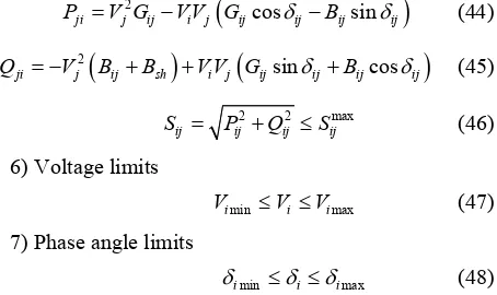
5) Transmission limits

The real and reactive power flow equations from bus-i

to bus-j can be written as:





2 _{cos sin}

ij i ij i j ij ij ij ij

P V G VV G  B 



ij

(42)







2 _{sin cos}

i ij sh i j ij ij ij ij

Q  V B B VV G  B 





2 _{cos sin}

(43)

The real and reactive power flow equations from bus-j

to bus-i can be written as:

ji j ij i j ij ij ij ij

P V G VV G  B 



(44)







2 _{sin cos}

ji j ij sh i j ij ij ij ij

Q  V B B VV G  B  (45)

2 2 max

ij ij ij ij

S  P Q S (46)

6) Voltage limits

min max

i i i

V V V (47) 7) Phase angle limits

min max

i i i

  





G G

2 2

t a

P Q V I

(48) 8) Reactive Power Capability Curves limit for genera-tors:

(49)

For hybrid market model, additional constraints to be satisfied are:

9) Equality constraints for bilateral transactions using transaction matrix GD are:

DB  GDij i sb



P (50)

GB ij

j bb

GD







P (51)

G  GB G

P P P_P (52) DB D

 

d

P P P_P



P



P

(53)



ACDF

 

fb

P P (54)



ACDF

 

fp

P P (55)

B P

 

f f

P P Pf (56)





max max

, ,

min ,

sb GB sb D

GD  P P_{B bb}

PDP = vector of pool demand

ation

rs based on AC load

ts of the seller and buyer buses, re-sp

on FACTS controllers:

(58) where uri = {0,1} is a binary variable defining

(57)

where GD = bilateral transaction matrix PDB = vector of bilateral demand

PGB = vector of bilateral gener

PGP = vector of pool generation

ACDF are the distribution facto flow approach [36].

s and b are the se ectively.

10) Limit SVC:

min max

* *

ri SVCi SVCi ri SVCi

u Q Q u Q

presence or absence of SVC.

TCSC:

max

0xcj ucj*xcj (59) where ucj = {0,1} is a binary variable defining presence or absence of TCSC in a branch.

UPFC:

max max

.*_T _T .*_T

u  u (60)

max max

.*Iq Iq .*Iq

u  u (61) max

0VT  u V. T (62)

u is thevector of binary variable (‘0’s an se

present work, impact of only one FACTS con-tro

d ‘1’s) repre-nting the presence or absence of UPFC with ‘1’s rep-resent presence and ‘0’s reprep-resent absence of FACTS devices.

In the

ller present in the system has been studied. However, more than one FACTS controller can be incorporated in the problem using the constraint on number of FACTS devices and can be represented as:

int max

FACTSi FACTSi FACTSi

N

 



The optimization problem is solved using the GAMS 21

for IEEE-24 bus

sys-devices for all meth-od

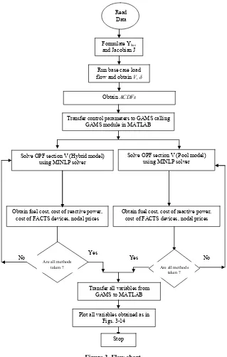
.3/DICOPT solver and utilizing interfacing with MAT-LAB 6.5 [28,29]. The flow chart for nodal price determi-nation with reactive and FACTS cost model is show in the Figure 3. The DICOPT model is based on the algo-rithm of outer approximation, equality relaxation, and augmented penalty approach [28].

6. Results and Discussions

tem for hybrid market model. The impact of three dif-ferent reactive cost models of generators’ reactive power cost estimation have been incorporated along with FACTS devices. The results have been obtained for dif-ferent cases for pool model also. The results obtained have been categorized as follows:

Reactive Power and FACTS Cost Models’ Impact on Nodal Pricing in Hybrid Electricity Markets 237

Transfer control parameters to GAMS calling GAMS module in MATLAB

Solve OPF section V (Hybrid model) using MINLP solver

Obtain fuel cost, cost of reactive power, cost of FACTS devices, nodal prices

Obtain fuel cost, cost of reactive power, cost of FACTS devices, nodal prices

Transfer all variables from GAMS to MATLAB

Plot all variables obtained as in Figs. 3-14

Solve OPF section V (Pool model) using MINLP solver

Stop Read Data

Formulate Ybus

and Jacobian J

Run base case load flow and obtain V, δ

Obtain ACDFs

Are all methods

taken ? Are all methods

taken ?

No Yes Yes No

Figure 3. Flow chart.

Case 2: Results with FACTS device (SVC) for all me-th

3: Results with FACTS device (TCSC) for all m

: Results with FACTS device (UPFC) for all m

ults for IEEE 24-bus test system (Bilateral M

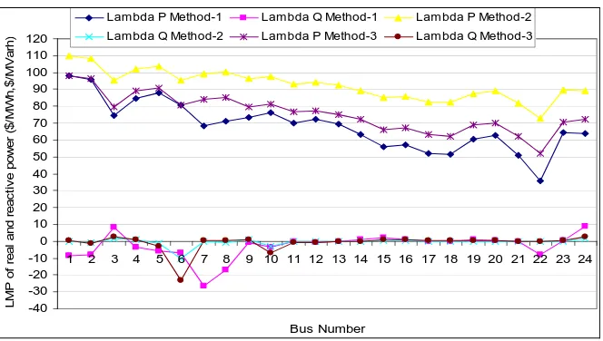
lots of the marginal cost for real and reactive po

thod-1, Method-2, Method-3) of reactive power cost

34.86 $/MWh with a m

ods Case ethods

Case 4 ethods

(a) Res odel)

The p

wer for Case 1 to Case 4 using different methods (Me-

model is shown in Figures 4 to 7.

It is observed from Figure 4 that the marginal cost of real power is minimum at bus 22 is

-40 -30 -20 -10 0 10 20 30 40 50 60 70

1 2 3 4 5 6 7 8 9 10 11 12 13 14 15 16 17 18 19 20 21 22 23 24

Bus number

LM

P

of

r

eal

and r

eac

ti

v

e

pow

er

($/

M

Wh,

$/

M

V

A

R

h)

Lambda P Method-1 Lambda Q Method-1

Lambda P Method-2 Lambda Q Method-2

Lambda P Method-3 Lambda Q Method-3

Figure 4. LMP of real and reactive power without any FACTS device for all methods (Case 1).

-40 -30 -20 -10 0 10 20 30 40 50 60

1 2 3 4 5 6 7 8 9 10 11 12 13 14 15 16 17 18 19 20 21 22 23 24

Bus Number

LM

P

of

r

e

al

an

d r

e

ac

ti

v

e

po

w

e

r (

$

/M

W

h

, $

/M

V

A

R

h)

Lambda P Method-1 Lambda Q Method-1

Lambda P Method-2 Lambda Q Method-2

Lambda P Method-3 Lambda Q Method-3

Figure 5. LMP of real and reactive power with SVC device for all methods (Case 2).

-30 -20 -10 0 10 20 30 40 50 60 70 80 90 100 110 120 130

1 2 3 4 5 6 7 8 9 10 11 12 13 14 15 16 17 18 19 20 21 22 23 24

Bus Number

LM

P

of

r

ea

l an

d r

eac

ti

v

e p

ow

er

($/

M

W

h,

$/

M

V

A

R

h

)

Lambda P Method-1 Lambda Q Method-1

Lambda P Method-2 Lambda Q Method-2

Lambda P Method-3 Lambda Q Method-3

Reactive Power and FACTS Cost Models’ Impact on Nodal Pricing in Hybrid Electricity Markets 239

-50

Bus Number -40

-30 -20 -10 0 10 20 30 40 50 60 70 80 90 100 110

1 2 3 4 5 6 7 8 9 10 11 12 13 14 15 16 17 18 19 20 21 22 23 24

LM

P

of

real

a

nd reac

ti

v

e pow

er ($/

M

W

H

, $/

M

V

A

R

h

Lambda P Method-1 Lambda Q Method-1 Lambda P Method-2 Lambda Q Method-2 Lambda P Method-3 Lambda Q Method-3

)

Figure 7. LMP of real and reactive power with UPFC for all methods (Case 4).

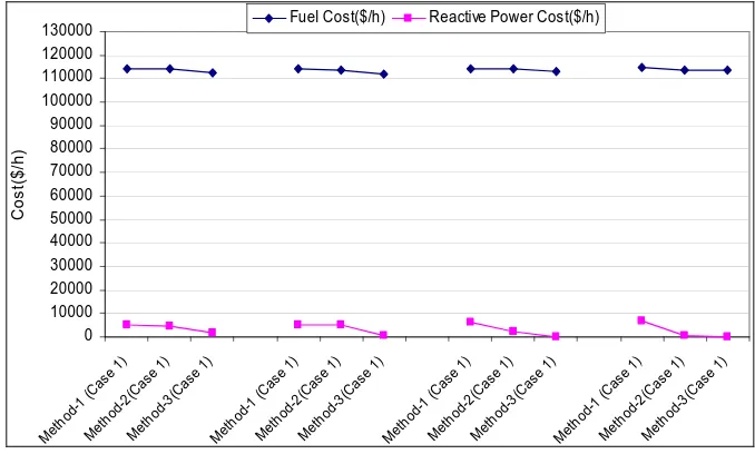
The reactive power nodal price is very small for me-thod-2 and for method-3 it is found higher and positive at all buses. Cost component of generators’ reactive power is obtained minimum using method-3. The fuel cost is obtained minimum for method-3 as observed from Fig-ure 8.

It is observed from Figure 5 that the marginal cost of real power is minimum at bus 22 with 34.74 $/MWh and with a maximum value of 53.85 $/MWh. The real power nodal price is observed to be lower for method-3 com-pared to method 1 and 2 with SVC. The nodal prices of both real and reactive power reduce for all methods with SVC. There is considerable reduction in reactive power nodal price with SVC. It is due to a support of reactive power to improve volt

stem. The minimum as

2 as compared to method 1 and 3. The nodal pr

is 40.88 $/MWh using Method-1 and is found with a

maximum value of 109.78 $/MWh for method-2. The real power nodal price is observed lower for method-1 compared to method-2 and 3. The cost component for reactive power is observed minimum for method-3. The fuel cost is found lower for method-3 as given in Figure 8. The fuel cost is observed higher than for Case-3 and lower for Case-1 and Case-2.

The cost component for UPFC is lower for method-3 due to its lower reactive power support compared to oth-er methods. The UPFC is optimally located on line be-tween buses 3 and 24. The cost component of UPFC is much larger than TCSC and SVC as UPFC is costlier than SVC and TCSC and reactive support obtained from UPFC is also higher compared to other FACTS devices. er with FACTS

de-the case without

plier is ne

found higher for method-3. Fuel cost is found lower us- age profile and reducing losses in a

fuel cost is obtained for method 3

The fuel cost is observed to be low vices for all methods compared to sy

shown in Figure 8. SVC is optimally located at bus 3. Cost component of SVC is obtained minimum for me-thod 1 as reactive power support is obtained minimum for this case. From Figure 6 (Case 3) with TCSC, it is found that the nodal prices for real power is lower for method

ices for real power are observed to increase with TCSC due to change in power flow patterns through lines. The nodal reactive power prices are observed to be higher with method-1 compared to method-2 and 3. The fuel cost is found lower using method-3. The reactive cost component is found lower for method-3 due to lower reactive support provided by TCSC. The cost component of TCSC is found minimum for method-1 due to lower reactive support provided by TCSC for this case.

With UPFC (Case 4), It is observed from Figure 7 that the marginal cost of real power is minimum at bus 22 and

FACTS controller. It is observed from Figure 9 that the cost component of FACTS devices is found lower for method 1 and UPFC cost component is higher compared to SVC and TCSC for all the methods.

The results obtained for nodal prices of real and reac-tive power for Case 1 to 4 using different methods of reactive power model is shown in Figures 10 to 13 for pool market model.

It is observed from Figure 10 (Case 1) that the mar-ginal cost of real power is minimum at bus 22 and the value is 32.927 $/MWh and with a maximum value 96.705 $/MWh. The marginal cost of reactive power is both positive and negative. The negative reactive power marginal cost represent that the Lagrange multi

0 10000 20000 30000 40000 50000

Met

hod-1 (C ase

1 60000 70000 80000 90000 100000 110000 120000 130000

)

Meth od-2

(Ca se 1

)

Meth od-3

(Cas e 1)

Met hod

-1(C ase 2

)

Meth od-2

(Cas e 2)

Met hod

-3(C ase 2

)

Meth od-1

(Cas e 3)

Meth od-2

(Ca se 3

)

Meth od-3

(Cas e 3)

Met hod

-1(C ase 4

)

Meth od-2

(Cas e 4)

Met hod

-3(C ase 4

)

C

o

s

t (

$

/h

)

Fuel Cost($/h) Reactive Pow er Cost($/h)

Figure 8. The fuel and reactive power cost ($/h) for all cases and all methods.

0 5 10 15 20 25 30

Meth

od-1(

Case

2)

Meth

od-2(C

ase 2

)

Meth

od-3(

Cas

e 2)

Meth

od-1(C

ase 3

)

Meth

od-2(

Cas

e 3)

Meth

od-3(

Cas

e 3)

Meth

od-1(

Cas

e 4)

Meth

od-2(

Cas

e 4)

Meth

od-3

(Case

4)

C

os

t of

F

A

C

T

S

c

ont

rol

le

r (

$/

h)

FACTS cost($/h)

Figure 9. The cost component for FACTS controllers ($/h) for all cases with all methods.

-50 -40 -30 -20 -10 0 10 20 30 40 50 60 70 80 90 100 110 120

1 2 3 4 5 6 7 8 9 10 11 12 13 14 15 16 17 18 19 20 21 22 23 24

Bus Number

Lambda P Method-1 Lambda Q Method-1 Lambda P Method-2 Lambda Q Method-2 Lambda P Method-3 Lambda Q Method-3

LM

P

of

real

and reac

ti

v

e pow

er

($/

M

W

h,

$/

M

V

A

rh

)

Reactive Power and FACTS Cost Models’ Impact on Nodal Pricing in Hybrid Electricity Markets 241

-50 -40 -30 -20 -10 0 10 20 30 40 50 60 70 80 90 100 110 120

1 2 3 4 5 6 7 8 9 10 11 12 13 14 15 16 17 18 19 20 21 22 23 24

Bus Number

LMP

of

r

eal

and r

eac

ti

v

e pow

er

(

$/

M

W

h,

$

/M

V

A

rh

)

Lambda P Method-1 Lambda Q Method-1 Lambda P Method-2 Lambda Q Method-2 Lambda P Method-3 Lambda Q Method-3

Figure 11. LMP of real and reactive power withSVC for all methods (Case 2).

-50 -40 -30 -20 -10 0 10 20 30 40 50 60 70 80 90 100 110 120

1 2 3 4 5 6 7 8 9 10 11 12 13 14 15 16 17 18 19 20 21 22 23 24

Bus Number

LMP

of

r

e

al

an

d r

e

ac

ti

v

e pow

er

(

$

/M

W

h,

$/

M

V

A

rh

)

Lambda P Method-1 Lambda Q Method-1 Lambda P Method-2

Lambda Q Method-2 Lambda P Method-3 Lambda Q Method-3

Figure 12. LMP of real and reactive power with TCSC for all methods (Case 3).

-40 -30 -20 -10 0 10 20 30 40 50 60 70 80 90 100 110 120

1 2 3 4 5 6 7 8 9 10 11 12 13 14 15 16 17 18 19 20 21 22 23 24

Bus Number

LMP

of

r

eal

and r

eac

ti

v

e pow

er

(

$/

M

W

h,

$/

M

V

ar

h

)

Lambda P Method-1 Lambda Q Method-1 Lambda P Method-2

Lambda Q Method-2 Lambda P Method-3 Lambda Q Method-3

ing method-3 as show

cost component is lower for method 3.

From Figure 11 it is observed that the marginal cost of real power is minimum at bus 22 and the values is 32.89 $/MWh and with a maximum value of 109.78 $/MWh for method 2. It is observed that marginal cost reduces at each bus with SVC. The impact on reactive power nodal prices is more prominent due to reactive support of SVC. We observe that marginal cost of reactive power is ob-tained minimum for method 2 however for method 3 it is found higher and positive at all buses. The upper and lower limits of QSVC have been considered as: 0.5 to 2.0

MVAR and SVC is optimally located at bus 3. The cost component of reactive power is lower for method-3. The cost component of SVC is found higher for method-3 as reactive support for this case is obtained higher com-pared to other cases. With SVC, the fuel cost is slightly lower compared to th

The results of the

e TCSC is opti-m

For Case 4 (with UPFC) is optimally connected be-tween bus 3 and 24. It is observed that the marginal cost of real power is minimum at bus 22 and is 42.006 $/MWh using Method 1 and with a maximum value 109.78 $/MWh using Method-2. The nodal prices are obtained lower for method-1. The reactive power cost component is lower for method-3. The cost component for UPFC is lower for method-1 due to lower reactive support obtained for this case. With UPFC, fuel cost is found to be more compared to fuel costs obtained with SVC and TCSC in all the methods as given in Figure 14. In comparison to TCSC, the nodal prices of real power are found lower at each bus. Reactive cost component is found lower for method 3 in all the cases. Cost compo-nent for UPFC is found higher compared to SVC and TCSC as shown in Figure 15.

s observed that with d with consideration odal prices are observed to be

n in Figure 14. The reactive power tained lower for method-3.

e case without SVC.

marginal cost for real and reactive

From all the four cases above, it i the FACTS devices cost models an power for Case-3 using different methods of reactive

power model is shown in Figure 12. Th

of reactive cost models, the n

different showing the effect of cost models on the marginal prices.

7. Conclusions

In this work, impact of reactive power cost model on nodal price for real and reactive power have been ob-tained. The cost model of FACTS devices have been incorporated to find their impact on real and reactive nodal price at each node. Based on the results, the fol-lowing conclusions are:

1) The nodal prices are found different with different methods and are found lower for method-2 in bilateral model for Case 1 and Case 2, however for Case 3 and 4, the nodal prices are found lower for method-1. For pool ally connected at line 7 between bus 3 and bus 24. For

TCSC, the limit of Xc is selected between 0.2 XL to 0.5

XL p.u. It is observed from Figure 12 that the marginal cost of real power is minimum at bus 22 and is 55.60 $/MWh with Method-1 and with a maximum value 113.68 $/MWh for Method-2. Nodal prices for real pow-er are found highpow-er with TCSC due to change in powpow-er flow pattern at all lines and are comparatively higher for method-2. The fuel cost is found lower for method-3 and slightly higher compared to Case 1 and 2 as given in the Figure 14. The cost component of TCSC is lower for method-1 as reactive support obtained from TCSC is lower for this case. The reactive cost component is

ob-Fuel Cost($/h) Reactive Power Cost($/h) 130000

0 10000 20000 30000 40000 50000 60000 70000 80000 90000 100000 110000 120000

Meth od-1

(Cas e 1

Co

s

t(

$

/h

)

)

Meth od-2

(Cas e 1)

Meth od-3

(Cas e 1)

Meth od-1

(Cas e 1)

Meth od-2

(Cas e 1)

Meth od-3

(Cas e 1)

Metho d-1

(Cas e 1)

Meth od-2

(Cas e 1)

Meth od-3

(Case 1)

Metho d-1

(Cas e 1)

Meth od-2

(Cas e 1)

Meth od-3

(Case 1)

Reactive Power and FACTS Cost Models’ Impact on Nodal Pricing in Hybrid Electricity Markets 243

0 5 10 15 20 25 30

Met hod-1

(Ca se 1

)

Met

hod-2(Ca se 1)

Met hod

-3(C ase

1)

Met ho

d-1 (C ase

1)

Met hod

-2(C ase

1)

Met

hod-3(C ase

1)

Met ho

d-1 (C ase

1)

Met ho

d-2(C ase

1)

Met

hod-3(C ase 1)

C

os

t of

F

A

C

T

S

c

o

nt

rol

ler

s

(

$/

h

)

FACTS cost($/h)

Figure 15. The cost component for FACTS controllers ($/h) for all cases with all methods

model, the nodal pric

with method 3 for Case 1 and Case 2 and lower with me-thod 1 for case 3 and case 4.

2) The reactive power nodal prices are both positive and negative at buses and with SVC are found lower due to its reactive support. With SVC the nodal prices for real power also reduces at all buses for all methods.

3) With UPFC, nodal prices are found lower compared to TCSC.

4) Cost components for reactive power are found lower for method-3 for all cases.

5) Cost component of UPFC is high compared to TCSC and SVC being costly device compared to SVC and TCSC.

6) Fuel cost is obtained minimum for method-3 for all the cases. With FACTS controllers, fuel costs are found to be lower compared to the case without FACTS con-trollers.

7) The nodal prices varies with the reactive cost

mod-herefore, th

rate transmission pricing and wheeling cost de

red in the model for accurate tra

REFERENCES

e Study Results,” IEEE , Vol. 6, No. 1, 1991, pp. 23-29. doi:org/10.1109/59.131043

.

es for real power are found lower Reactive Power: Theory and Cas Transactions on Power Systems

[2] N. Dandachi, M. Rawlins, O. Alsac, M. Paris and B. Stott, “OPF for Reactive Power Transmission Pricing on The NGC System,” IEEE Transactions on Power Systems, Vol. 11, No. 1, 1996, pp. 226-232.

doi:org/10.1109/59.486099

[3] M. Einborn and R. Siddiqi, “Electricity Transmission Pricing and Technology,” Kluwer Academic Publishers, Dordrecht, 1996.

[4] F. C. Schweppe, M. C. Caramanis, R. D. Tabors and R. E. Bohn, “Locational Based Pricing of Electricity,” Kluwer Academic Publishers, Dordrecht, 1988.

[5] M. Rivier and I. Perez-Ariaga, “Computation and De-composition of Location Based Price for Transmission Pricing,” Proceedings of 11th Power Systems

Computa-tion Conference, Avignon, France, 3

Septem-eering Model for

n,” IEEE Transactions on Power Systems, Vol. 12, No. els considered for study and cost model of FACTS

de-vices also plays an important role for variation in nodal prices.

Based on the results, it is concluded that reactive cost models have considerable impact on LMPs of real and reactive power at each bus. Cost model of FACTS de-vices also have noticeable impact on LMPs. T

e ISO must consider the appropriate reactive cost mod-els for accu

termination for better market operation. FACTS cost component can not be igno

nsmission pricing due to their impact on LMPs.

[1] M. L. Baughman and S. N. Siddiqi, “Real Time Pricing of

0 August-3 ber, 1993.

[6] D. Ray and F. Alvarado, “Use of Engin

Economic Analysis in the Electric Utility Industry,” Pre-sented at the Advanced Workshop on Regulation and Public Utility Economics, Rutgers University, 25-27 May, 1988.

[7] A. A. El-Keib and X. Ma, “Calculating the Short-Run Marginal Costs of Active and Reactive Power Produc-tio

2, 1997, pp. 559-565. doi:org/10.1109/59.486099

[8] Y. Z. Li and A. K. David, “Wheeling Rates of Reactive Flow under Marginal Cost Theory,” IEEE Transactions on Power Systems, Vol. 10, No. 3, 1993.

[9] A. Zobian and M. Ilic, “Unbundling of Transmission and Ancillary Services,” IEEE Transactions on Power Sys-tems, Vol. 12, No. 1, 1997, pp. 539-548.

pp. 217-224.

[11] M. L. Baughman, S. N. Siddiqi and J. W. Jarnikau, “Ad-vanced Pricing in Electrical Systems-Part II,” IEEE Transactions on Power Systems, Vol. 12, No. 1, 1997, pp. 496-502.doi:org/10.1109/59.575803

[12] K. Xie, Y. H. Song, J. Stonham, E. Yu and G. Liu, “De-composition Model and Interior Point Methods for Opti-mal Spot Pricing of Electricity in Deregulated Environ-ments,” IEEE Transactions on Power Systems, Vol. 15, No. 1, 2000, pp. 39-50.doi:org/10.1109/59.852099 [13] D. Chattopadhyaya, K. Bhattacharya and J. Parikh,

“Op-timal Reactive Power Planning and Its Spot Pricing: An Integrated Approach,” IEEE Transactions on Power Sys-tems, Vol. 10, No. 4, 1995, pp. 2014-2019.

doi:org/10.1109/59.476070

[14] J. Y. Choi, S. Rim and J. Park, “Optimal Real Time Pric-ing of Real and Reactive Powers,” IEEE Transactions on Power Systems, Vol. 13, No. 4, 1998, pp. 1226-1231. doi:org/10.1109/59.736234

[15] S. Hao and A. Pepalexopolous, “A Reactive Power Pric-ing and Management,” IEEE Transactions on Power Sys-tems, Vol. 12, No. 1, 1997, pp. 95-104.

doi:org/10.1109/59.574928

[16] J. W. Lamont and R. Fu, “Cost Analysis of Reactive Power Support,” IEEE Transactions on Power Systems, Vol. 13, No. 3, 1999, pp. 890-898.

doi:org/10.1109/59.780900

[17] M. Muchayi and M. E. El-Hawary, “A Summary of Algo-rithms in Reactive Power Pricing,” Electric Power and System Research, Vol. 21, 1999, pp. 119-124.

doi:org/10.1016/S0142-0615(98)00039-8

[18] V. M. Dona and A. N. Paredes, “Reactive Power Pricing in Competitive Electric Markets Using Transmission Losses Function,” IEEE Porto Power Tech Conference, Porto, 10-13 September 2001.

[19] J. B. Gill, T. G. S. Roman, J. J. A. Rioa and P. S. Martin, “Reactive Power Pricing: A Conceptual Framework for Remuneration and Charging Procedures,” IEEE Transac-tions on Power Systems, Vol. 15, No. 2, 2000, pp. 483- 489.doi:org/10.1109/59.867129

[20] V. L. Paucar and M. J. Rider, “Reactive Power Pricing in Deregulated Electrical Markets Using Methodology Based on Theory of Marginal Costs,” Proceedings of IEEE PES General Meeting, Vancouver, 2001.

[21] M. J. Rider and M. L. Paucar, “Application of Nonlinear Reactive Power Pricing Model for Competitive Electric Markets,” IEE Proceedings—Generation, Transmission, Distribution, Vol. 151, No. 3, 2004, pp. 407-414.

doi:org/10.1049/ip-gtd:20040385

Y. Zhao, M. R. Irving and Y. Song “A Cost Allo

[22] cation

and Pricing Method for Reactive Power Services in the New Deregulated Electricity Market Environment,” Pro-ceedings of IEEE Transmission and Distribution Confer-ence, Dalian, August 2005.

L. J. Cai and István Erlich, “

[23] Optimal Choice and

Alloca-tion of FACTS Devices Using Genetic Algorithms,” Pro-ceedings of ISAP, Intelligent Systems Application to

Power Systems, 2003, Lemnos, 31 August-3 Septem

2003. ber,

Energy Systems, -118.

Electric Utility De-g and Power TechnoloDe-gies,

nd Energy 36.

[24] E. J. de Olivera, J. W. M. Lima and J. L. R. Pereira, “Flexible AC Transmission Devices: Allocation and Trans- mission Pricing,” Electric Power and

Vol. 21, No. 2, 1999, pp. 111

[25] S. C. Srivastava and R. K. Verma, “Impact of FACTS Devices on Transmission Pricing in a Deregulated Mar-ket,” International Conference on

regulation and Restructurin

DRPT, London, 4-7April 2000, pp. 642-648.

[26] G. B. Shrestha and W. Feng, “Effects of Series Compen-sation on Spot Price Markets,” Electric Power a

Systems, Vol. 27, No. 5-6, 2005, pp. 428-4 doi:org/10.1016/j.ijepes.2005.03.001

[27] S. Chanana and A. Kumar, “Effect of Optimally Located FACTS Devices on Active and Reactive Power Price in Deregulated Electricity Markets,” IEEE Power India Con- ference, New Delhi, 10-12 April 2006.

[28] G. Hamoud, “Feasibility Assessment of Simultaneous Bilateral Transactions in a Deregulated Environment,” IEEE Transactions on Power systems, Vol. 15, No. 1, 2000, pp. 22-26.doi:org/10.1109/59.852096

pp. 1020- [29] J. W. M. Cheng, F. D. Galiana and D. T. McGills,

“Stud-ies of Bilateral Contracts with Respect to Steady State Security in a Deregulated Environment,” IEEE Transac-tions on Power Systems, Vol. 13, No. 3, 1998,

1025. http://dx.doi.org/10.1109/59.709092

[30] J. W. M. Cheng, D. T. McGills and F. D. Galiana, “Prob-abilistic Security Analysis of Bilateral Transactions in a Deregulated Environment,” IEEE Transactions on Systems, Vol. 14, No. 3, 1999, pp.

Power 1153-1159.

doi:org/10.1109/59.780948

[31] F. D. Galiana and M. Ilic, “A Mathematical Framework for the Analysis and Management of Power Transactions under Open Access,” IEEE Transactions on Power Sys-tems, Vol. 13, No. 2, 1998, pp. 681-687.

doi:org/10.1109/59.667400

[32] GAMS—The Solver Manuals, GAMS Development Cor-poration, March 2001.

[33] M. C. Ferris, “MATLAB and GAMS: Interfacing Opti-mization and Visualization Software,” 10 August 1999.

ol. PAS-98, 1979, pp.

36, No. 6, [34] “IEEE Reliability Test System, A report prepared by the Reliability Test System Task Force of the Applications of Probability Methods Subcommittee,” IEEE Transactions on Power Apparatus and Systems, V

2047-2054.

[35] A. K. Sharma and S. Chanana, “New Multiobjective Op-timization Problem for Secure Bilateral Transaction De-termination with UPFC in Hybrid Electricity Markets,” Electric Power Components and Systems, Vol.

2008, pp. 555-574. doi:org/10.1080/15325000701801561 [36] G. Shaoyun, “Optimal Power System Operation and

Con-trol Incorporating FACTS Devices,” Ph.D. The