http://wrap.warwick.ac.uk
Original citation:
Garcke, Harald, Lam, Kei Fong and Stinner, Björn. (2014) Diffuse interface modelling of
soluble surfactants in two-phase flow. Communications in Mathematical Science,
Volume 12 (Number 8). pp. 1475-1522. ISSN 1539-6746
Permanent WRAP url:
http://wrap.warwick.ac.uk/57676
Copyright and reuse:
The Warwick Research Archive Portal (WRAP) makes this work by researchers of the
University of Warwick available open access under the following conditions. Copyright ©
and all moral rights to the version of the paper presented here belong to the individual
author(s) and/or other copyright owners. To the extent reasonable and practicable the
material made available in WRAP has been checked for eligibility before being made
available.
Copies of full items can be used for personal research or study, educational, or not-for
profit purposes without prior permission or charge. Provided that the authors, title and
full bibliographic details are credited, a hyperlink and/or URL is given for the original
metadata page and the content is not changed in any way.
Publisher’s statement:
“First published in Communications in Mathematical Science, Volume 12 (Number 8)
2014 published by International Press.”
© International Press. All rights reserved.
A note on versions:
The version presented here may differ from the published version or, version of record, if
you wish to cite this item you are advised to consult the publisher’s version. Please see
the ‘permanent WRAP url’ above for details on accessing the published version and note
that access may require a subscription.
IN TWO-PHASE FLOW∗
HARALD GARCKE †, KEI FONG LAM ‡, AND BJ ¨ORN STINNER §
Abstract. Phase field models for two-phase flow with a surfactant soluble in possibly both fluids are derived from balance equations and an energy inequality so that thermodynamic consistency is guaranteed. Via a formal asymptotic analysis, they are related to sharp interface models. Both cases of dynamic as well as instantaneous adsorption are covered. Flexibility with respect to the choice of bulk and surface free energies allows us to realise various isotherms and relations of state between surface tension and surfactant. Some numerical simulations display the effectiveness of the presented approach.
Key words. Two-phase flow, surfactant, phase field model, adsorption isotherm
subject classifications. 35R35, 35R01, 76T99, 76D45, 35C20, 35Q35
1. Introduction Surface active agents (surfactants) reduce the surface tension of fluid interfaces and, via surface tension gradients, can lead to tangential forces re-sulting in the Marangoni effect. Biological systems take advantage of their impact on fluids with interfaces, but surfactants are also important for industrial applications such as processes of emulsification or mixing. While often much experience and knowl-edge is available on how surfactants influence the rheology of multi-phase fluids, the goal is to understand how exactly the presence of a surfactant influences coalescence and segregation of droplets.
Surfactants can be soluble in at least one of the fluid phases and the exchange of surfactants between the bulk phases and the fluid interfaces is governed by the process of adsorption and desorption. Ward and Tordai [55] derived a time-dependent relation for the surfactant density at the interface and the surfactant density at the adjacent bulk phase (known as the sub-layer or sub-surface). To compute the interfacial density, a closure relation between the two quantities has been proposed in the form of several different equilibrium isotherms [18, 33, 32], where the underlying assumption is that the interface is in equilibrium with the sub-layer at all times. This corresponds to the case of diffusion-limited adsorption studied in Diamant and Andelman [16], where the process of adsorption to the interface is fast compared to the kinetics in the bulk phases. However, instantaneous adsorption is not valid in the context of ionic surfactant systems [16] or when the diffusion is not limited to a thin layer [12, 13, 14]. Therefore, we would like to be able to account for non-instantaneous adsorption in our models.
Two-phase flow with surfactant is classically modelled with moving hypersurfaces describing the interfaces separating the two fluids. We will derive the following sharp interface model for a domain Ω containing two fluids of different mass densities. We denote by Ω(1)(t), Ω(2)(t) the domains of the fluids which are separated by an interface
∗
†address: Fakult¨at f¨ur Mathematik, Universit¨at Regensburg, 93040 Regensburg, Germany, (email:
‡address: Mathematics Institute, Zeeman Building, University of Warwick, Coventry, CV4 7AL,
UK, (email: [email protected]).
§address: Mathematics Institute and Centre for Scientific Computing, University of Warwick,
Γ(t):
∇·v=0, in Ω(i)(t), (1.1)
∂t(ρ(i)v) +∇·(ρ(i)v⊗v) =∇·
(
−pI+ 2η(i)D(v)
)
, in Ω(i)(t), (1.2)
∂t•c(i)=∇·(Mc(i)∇G′i(c(i))), in Ω(i)(t), (1.3) [v]21=0, v·ν=uΓ, on Γ(t), (1.4) [pI−2η(i)D(v)]21ν=σ(cΓ)κν+∇Γσ(cΓ), on Γ(t), (1.5)
∂t•cΓ+cΓ∇Γ·v−∇Γ·(MΓ∇Γγ′(cΓ)) =[Mc(i)∇G′i(c
(i))]2
1ν, on Γ(t), (1.6)
α(i)(−1)iMc(i)∇G′i(c(i))·ν,=−(γ′(cΓ)−Gi′(c(i))) on Γ(t). (1.7)
Herevdenotes the fluid velocity,ρ(i)is the constant mass density for fluidi,η(i)is the viscosity of fluidi, D(v) =1
2(∇v+ (∇v)⊥) is the rate of deformation tensor, pis the pressure,I is the identity tensor,∂t•(·) =∂t(·) +v·∇(·) is the material derivative,c(i)
is the bulk density of surfactant in fluidi,Mc(i)is the mobility of surfactants in fluid
i,Gi(c(i)) is the bulk free energy density associated to the bulk surfactant in fluidi.
On the interface,uΓ is the normal velocity, ν is the unit normal on Γ pointing into Ω(2), cΓ is the interfacial surfactant density,σ(cΓ) is the density dependent surface tension, κ is the mean curvature of Γ, ∇Γ is the surface gradient operator, ∇Γ· is the surface divergence,MΓ is the mobility of the interfacial surfactants,γ(cΓ) is the free energy density associated to the interfacial surfactant, and α(i)≥0 is a kinetic factor that relates to the speed of adsorption. The above model satisfies the second law of thermodynamics in an isothermal situation in the form of an energy dissipation inequality.
Equations (1.1) and (1.2) are the classical incompressibility condition and mo-mentum equation, respectively. The mass balance equation for bulk surfactants is given by (1.3). Equation (1.4) states that the interface is transported with the flow and that not only the normal components but also the tangential components of the velocity field match up. The force balance on the interface (1.5) relates the jump in the stress tensor across the interface to the surface tension force and the Marangoni force at the interface. The mass balance of the interfacial surfactants is given by (1.6), and the closure condition (1.7) tells us whether adsorption is instantaneous (α(i)= 0, an isotherm is obtained) or dynamic (α(i)>0, the mass flux into the interface is proportional to the difference in chemical potentials).
The model studied in [9, 10] bears the most resemblance to the above model, where the setting of these papers is the diffusion-limited regime with a surfactant which is soluble in one phase only and (1.7) is replaced by the relation
γ′(cΓ) =G′(c) ⇐⇒ cΓ=g(c) := (γ′)−1(G′(c)), (1.8)
in which g plays the role of the equilibrium isotherm and whereG is the bulk free energy of the phase in which the surfactant is soluble. Our approach is based on a free energy formulation, originated from [16, 17], where we gain access to equilibrium isotherms by setting α(i)= 0 and choosing suitable functions for γ andGi.
Further-more, for positive values ofα(i)we are able to include the dynamics of non-equilibrium adsorption.
the interface using various numerical methods [58, 28, 57, 36, 44, 30]. However, the sharp interface description breaks down when topological changes occur. Phenomena such as breakup of fluid droplets, reconnection of fluid interfaces, and tip-streaming driven by Marangoni forces [21, 35, 34] involve changes in the topology of the inter-face. Numerically, complications also arise when the shape of the interface becomes complicated or exhibits self-intersections. These difficulties have led to the develop-ment of diffuse interface or phase field models to provide an alternative description of fluid/fluid interfaces.
At the core of these models, the sharp interface is replaced by an interfacial layer of finite width and an order parameter is used to distinguish between the bulk fluids and interfacial layer. The order parameter takes distinct constant values in each of the bulk fluids and varies smoothly across the narrow interfacial layer. The original sharp interface can then be represented as the zero level set of the order parameter, thus allowing different level sets to exhibit different topologies.
The width of the interfacial layer is characterised by the length scale over which the order parameter varies from its values at the bulk regions. The phase field model can be related to the sharp interface model in the asymptotic limit in which this width is small compared to the length scales associated to the bulk regions. Hence one can also view the phase field methodology purely as a tool for approximating the sharp interface equations. If the objective is to ensure that, in the limit of vanishing interfacial thickness, certain sharp interface models are recovered then there is a lot of freedom in constructing phase field models to meet one’s needs (see e.g. [37]).
The review [4] provides an overview on diffuse interface methods in the context of fluid flows. In [26, 27] it was already proposed to combine a Cahn-Hilliard equation for distinguishing the two phases with a Navier-Stokes system. An additional term was included in the momentum equation to model the surface contributions to forces. In the case of different densities, Lowengrub and Truskinovsky [41] derived quasi-incompressible models, where the fluid velocity is not divergence free. On the other hand, Abels, Garcke, and Gr¨un [1] derived a thermodynamically consistent diffuse interface model for two-phase flow with different densities and with solenoidal fluid velocities. Following the derivation in [1], we will derive three diffuse interface models, which approximate the sharp interface models in the diffuse-limited regime.
More precisely, for the case of non-instantaneous adsorption (α(i)>0), we will derive the following model (denoted Model A):
∇·v= 0, (1.9)
∂t(ρv) +∇·(ρv⊗v) =∇·
(
−pI+ 2η(φ)D(v) +v⊗ρ(2)−2ρ(1)m(φ)∇µ )
(1.10)
+∇·(σ(cΓ)(δ(φ,∇φ)I−Wε∇φ⊗∇φ)),
∂t•φ=∇·(m(φ)∇µ), (1.11)
µ+∇·(Wεσ(cΓ)∇φ) =W
ε σ(c
Γ)W′(φ) + ∑
i=1,2
ξ′i(φ)(Gi(c(i))−G′i(c(i))c(i)), (1.12)
∂•t(ξi(φ)c(i)) =∇·(Mc(i)(c
(i))ξ
i(φ)∇G′i(c
(i))) (1.13)
+α1(i)δ(φ,∇φ)(γ′(c
Γ)−G′
i(c
(i))), i= 1,2,
∂t•(δ(φ,∇φ)cΓ) =∇·
(
MΓ(cΓ)δ(φ,∇φ)∇γ′(cΓ)
)
(1.14)
−δ(φ,∇φ)∑
i=1,2 1
α(i)(γ′(c
Γ)−G′
i(c
Here εis a length scale associated with the interfacial width, φis the order param-eter that distinguishes the two bulk phases. In fact φ takes values close to ±1 in the two phases and rapidly changes from −1 to 1 in an interfacial layer. The func-tionsξi(φ) and δ(φ,∇φ) act as regularisation to the indicator functions of Ω(i) and
Γ, respectively, whileWis a constant related toδ(φ,∇φ). Equations (1.9) and (1.10) are the incompressibility condition and the phase field momentum equations, respec-tively. Equation (1.11) together with (1.12) governs how the order parameter evolves and equations (1.13) and (1.14) are the bulk and interfacial surfactant equations, respectively.
We derive two additional models for instantaneous adsorption (α(i)= 0): Model B models the case where the surfactant is soluble in only one of the bulk phases. It consists of (1.9)−(1.12) and replaces the bulk and interface surfactant equations (1.13), (1.14) with
∂t•(ξ(φ)c+δg(c))−∇·(M(c)ξ(φ)∇G′(c))−∇·(MΓ(g(c))δ∇G′(c)) = 0, (1.15)
whereg(c) is the adsorption relation between interface and bulk densities as in (1.8). The case where the surfactant is soluble in both bulk phases is covered by Model C, which consists of (1.9)−(1.12) and
∂t•(ξ1(φ)c(1)(q) +ξ2(φ)c(2)(q) +δcΓ(q))−∑
i=1,2
∇·(Mi(c(i)(q))ξi(φ)∇q) (1.16)
−∇·(MΓ(cΓ(q))δ∇q) = 0.
Here, qdenotes a chemical potential where, as will be discussed in Section 3, we can express the surfactant densities as functions ofq.
The Model A is related to the approach in [49]. We modify the approach of [49] in such a way that an energy inequality is valid and such that we recover the isotherm relations for adsorption phenomena in the limit of instantaneous adsorption. We deepen the asymptotic analysis in that it works with the original equation for the surface quantity and does not require the assumption of extending the surface quantity continuously in the normal direction. Phase field models of surfactant adsorption that utilise the free energy approach of [16, 17] can be traced back to the models of [53, 52, 54], where the latter is extended in [40] and solved using lattice Boltzmann methods. The issue of ill-posedness of the model is discussed in [20] and three alternatives have been suggested. Phase field models that look into the behaviour of equilibrium configurations of fluid-surfactant systems can be found in [23, 51] and a detailed comparison of previous phase field models can be found in [38].
2. Sharp interface model
2.1. Balance equations We consider a domain Ω⊂Rd,d= 1,2,3, containing
two immiscible, incompressible Newtonian fluids with possibly different constant mass densitiesρ(i), i= 1,2. The domain occupied by the fluid with densityρ(i) is labelled as Ω(i)⊂R×Rd, where we set Ω(i)(t) :={x∈Ω;(t,x)∈Ω(i)}. The two domains are separated by an interface Γ which is a hypersurface inR×Rd such that Γ(t)∩∂Ω =∅, where Γ(t) :={x∈Ω;(t,x)∈Γ}. A surfactant is present which alters the surface tension by adsorbing to the fluid interface and, provided it is soluble in the corresponding fluid, it is subject to diffusion in the phases Ω(i). We denote the fluid velocity field byv, the pressure byp, the bulk surfactant densities byc(i),i= 1,2, and the interface surfactant density bycΓ.
Balance of mass and linear momentum inside the phases lead to the following equations:
∇·v= 0, ∂t(ρ(i)v) +∇·(ρ(i)v⊗v) =∂t•(ρ
(i)v) =∇·T(i),
where ∂•t denotes the material derivative and T(i), i= 1,2, is the symmetric stress tensor (due to conservation of angular momentum). These equations hold in Ω(1)(t)∪ Ω(2)(t). We assume that the two fluids do not undergo phase transitions and the phase boundary Γ(t) is purely transported with the flow which we also assume has no-slip at the interface, hence the tangential velocities match:
[v]21= 0, v·ν=uΓ.
Here [·]21 denotes the jump of the quantity in brackets across Γ from Ω(1) to Ω(2),νis the unit outward normal of Γ(t) pointing into Ω(2)(t), and uΓ is the normal velocity of the interface.
LetV(t) be an arbitrary material test volume in Ω with external unit normalνext
ofV(t)∩Ω. IfV(t)∩Γ(t) is non-empty then we denote its external unit co-normal by µand write νext(i) for the external unit normal of V(t)∩Ω(i)(t), i= 1,2. In the bulk fluid regions, surfactants will be subjected to transport mechanisms consisting of only diffusion and convection. Hence, mass balance for bulk surfactants in a material test volumeV(t) away from the interface Γ(t) yields
d dt
∫
V(t)
c(i)=−
∫
∂V(t)
Jc(i)·νext,
where Jc(i) is the molecular flux. By Reynold’s transport theorem and using that ∇·v= 0, this leads to the pointwise law
∂t•c(i)+∇·Jc(i)= 0, i= 1,2. (2.1)
For a test volumeV(t) intersecting Γ(t), we postulate
d dt
∑
i=1,2
∫
V(t)∩Ω(i)(t) c(i)+
∫
V(t)∩Γ(t)
cΓ
(2.2)
=∑
i=1,2
∫
∂(V(t)∩Ω(i)(t))\Γ(t)
−Jc(i)·νext+
∫
∂(V(t)∩Γ(t))
whereJΓ is the interfacial molecular flux, tangential to Γ. Using Reynold’s transport theorem, the surface transport theorem and the surface divergence theorem (see [6]) we obtain
d dt
∑
i=1,2
∫
V(t)∩Ω(i)(t) c(i)+
∫
V(t)∩Γ(t)
cΓ = 2 ∑ i=1 ∫
V(t)∩Ω(i)(t) ∂•tc
(i) +
∫
V(t)∩Γ(t)
( ∂t•c
Γ
+cΓ∇Γ·v
)
for the left hand side and
∑
i=1,2
−
∫
∂(V(t)∩Ω(i)(t))\Γ(t)
Jc(i)·νext−
∫
∂(V(t)∩Γ(t)) JΓ·µ
=∑
i=1,2
−
∫
∂(V(t)∩Ω(i)(t))
Jc(i)·ν
(i)
ext−
∫
V(t)∩Γ(t) ([Jc(i)]
2
1ν+∇Γ·JΓ)
for the right hand side. Hence, using (2.1) the mass balance (2.2) yields the following pointwise law for the interfacial surfactant:
∂t•cΓ+cΓ∇Γ·v=−∇Γ·JΓ+qAD,
whereqAD=−[J
(i)
c ]21νis the mass flux for the transfer of surfactant to the interface from the adjacent sub-layers. When the mass flux qAD is zero and the interfacial
molecular flux is modelled by Fick’s law,JΓ=−Ds∇ΓcΓ, we obtain the mass balance equation in [56].
2.2. Energy inequality We postulate a total energy of the form
∫
Ω(1)(t)
[ρ(1)2 |v|2+G1(c(1))] +
∫
Ω(2)(t)
[ρ(2)2 |v|2+G2(c(2))] +
∫
Γ(t)
γ(cΓ), (2.3)
whereG1,G2are the bulk free energy densities, andγis a surface free energy density. We assume that γ′′>0 and G′′i >0. The Legendre transform of the surface energy density then is well defined, and the density dependent surface tensionσ(cΓ) is defined as
σ(cΓ) :=γ(cΓ)−cΓγ′(cΓ). (2.4)
LetV(t) be an arbitrary material test volume. Then
d dt ( 2 ∑ i=1 ∫
V(t)∩Ω(i)(t)
(ρ(2i)|v|2+Gi(c(i))) +
∫
V(t)∩Γ(t)
γ(cΓ)
) = 2 ∑ i=1 ∫
V(t)∩Ω(i)(t) (
ρ(i)v·∂t•v+Gi′(c(i))∂•tc(i) )
+
∫
V(t)∩Γ(t)
(
γ′(cΓ)∂t•cΓ+γ(cΓ)∇Γ·v
) = 2 ∑ i=1 ∫
V(t)∩Ω(i)(t) (
∇·((T(i))⊥v−Gi′(c(i))Jc(i))−T(i):∇v+∇G′i(c(i))·Jc(i)
)
+
∫
V(t)∩Γ(t)
= 2
∑
i=1
∫
V(t)∩Ω(i)(t)
−T(i):∇v+∇G′i(c(i))·Jc(i)+
∫
∂(V(t)∩Γ(t))
−γ′(cΓ)JΓ·µ
+ 2
∑
i=1
∫
∂(V(t)∩Ω(i)(t))\Γ(t)
((T(i))⊥v−G′i(c(i))Jc(i))·νext
+
∫
V(t)∩Γ(t)
((T(1))⊥v−G′1(c (1)
)Jc(1))·ν+ ((T
(2)
)⊥v−G′2(c (2)
)Jc(2))·(−ν)
+
∫
V(t)∩Γ(t)
JΓ·∇Γγ′(cΓ) +γ′(cΓ)(Jc(1)·ν−J
(2)
c ·ν) +σ(c
Γ)∇ Γ·v.
Decomposing the velocity fieldv on Γ(t) into its normal and tangential components,
v=uΓν+vτ,
then gives
∫
V(t)∩Γ(t)
σ(cΓ)∇Γ·(uΓν+vτ) =
∫
V(t)∩Γ(t)
σ(cΓ)(∇| {z }ΓuΓ·ν
=0
+u| {z }Γ∇Γ·ν
−κuΓ
+∇Γ·vτ)
=
∫
V(t)∩Γ(t)
−σ(cΓ)κuΓ−∇Γσ(cΓ)·v+
∫
∂(V(t)∩Γ(t))
σ(cΓ)vτ·µ,
where κ=−∇Γ·ν is the mean curvature and we have used integration by parts to obtain the last equality. Altogether we have
d dt ( 2 ∑ i=1 ∫
V(t)∩Ω(i)(t)
[ρ(2i)|v|2+Gi(c(i))] +
∫
V(t)∩Γ(t)
γ(cΓ)
) = 2 ∑ i=1 ∫
∂(V(t)∩Ω(i)(t))\Γ(t)
((T(i))⊥v−G′i(c(i))Jc(i))·νext
+
∫
∂(V(t)∩Γ(t))
(
−γ′(cΓ)JΓ·µ+σ(cΓ)vτ·µ
) + 2 ∑ i=1 ∫
V(t)∩Ω(i)(t) (
−T(i):∇v+∇Gi′(c(i))·Jc(i)
)
+
∫
V(t)∩Γ(t)
JΓ·∇Γγ′(cΓ)
+
∫
V(t)∩Γ(t)
(
(γ′(cΓ)−G1′(c(1)))Jc(1)·ν−(γ′(cΓ)−G2′(c(2)))Jc(2)·ν
)
+
∫
V(t)∩Γ(t)
(
T(1)ν·v−T(2)ν·v−σ(cΓ)κv·ν−∇Γσ(cΓ)·v
) .
Hence, if
Jc(i)·∇G′i(c(i))≤0, in Ω(i)(t), i= 1,2,
JΓ·∇Γγ′(cΓ)≤0, on Γ(t), (Jc(1)·ν)(γ′(cΓ)−G′1(c(1)))≤0, on Γ(t),
(−Jc(2)·ν)(γ′(cΓ)−G′2(c(2)))≤0, on Γ(t),
(−[T]21ν−σ(c Γ
)κν−∇Γσ(cΓ))·v≤0, on Γ(t),
then we obtain the following energy inequality:
d dt
( 2
∑
i=1
∫
V(t)∩Ω(i)(t)
(ρ(2i)|v|2+Gi(c(i))) +
∫
V(t)∩Γ(t)
γ(cΓ)
)
≤
2
∑
i=1
(∫
∂(V(t)∩Ω(i)(t))\Γ(t)
((T(i))⊥v−G′i(c(i))Jc(i))·νext
)
+
∫
∂(V(t)∩Γ(t))
(
−γ′(cΓ)JΓ·µ+σ(cΓ)vτ·µ
) ,
where the right hand side represents the working on the arbitrary material test volume
V(t) and the inequality indicates that the dissipation is non-positive, thus guarantee-ing thermodynamic consistency [24, 26].
2.3. General model We make the following constitutive assumptions:
Jc(i)=−Mc(i)(c(i))∇G′i(c(i)),
JΓ=−MΓ(cΓ)∇Γγ′(cΓ),
α(i)(cΓ,c(i))(−1)i+1Jc(i)·ν=−(γ′(cΓ)−G′i(c(i))), (2.5) T(i)=−pI+ 2η(i)D(v),
−[T]21ν=σ(c Γ
)κν+∇Γσ(cΓ),
whereMc(i)(c(i))>0,MΓ(cΓ)>0, andα(i)(cΓ,c(i))≥0.
The formulation presented in (2.5) utilises a free energy approach, first applied to the kinetics of surfactant adsorption in [16, 17], to model instantaneous adsorption kinetics. At adsorption/desorption equilibrium, the chemical potentials γ′(cΓ) and
G′(c) must be equal [59, 40, 54] and thus this approach allows us to cover the ad-sorption isotherms often used in the literature by selecting suitable functional forms forγ andG. Hence, α(i)>0 can be seen as a kinetic factor which relates the speed of adsorption to the interface or desorption from the interface to the deviation from local thermodynamical equilibrium. Let us summarise the governing equations of the general model for two-phase flow with soluble surfactant:
Balance equations in Ω(i)(t), i= 1,2 :
∇·v= 0, (2.6)
∂t(ρ(i)v) +∇·(pI−2η(i)D(v) +ρ(i)v⊗v) = 0, (2.7)
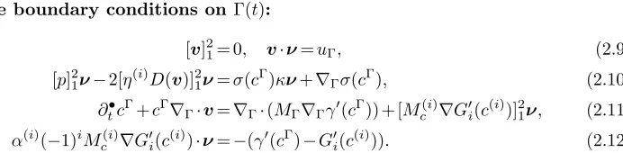
Free boundary conditions on Γ(t):
[v]21= 0, v·ν=uΓ, (2.9) [p]21ν−2[η
(i)
D(v)]21ν=σ(c Γ
)κν+∇Γσ(cΓ), (2.10)
∂t•cΓ+cΓ∇Γ·v=∇Γ·(MΓ∇Γγ′(cΓ)) + [Mc(i)∇G′i(c
(i))]2
1ν, (2.11)
α(i)(−1)iMc(i)∇G′i(c(i))·ν=−(γ′(cΓ)−G′i(c(i))). (2.12)
In this model, the surface tensionσ:R+→R+ is a (usually decreasing) function of the surfactant densitycΓ. The phenomenon known as Marangoni effect, where tan-gential stress at the phase boundary leads to flows along the interface, is incorporated into the model via the surface gradient of σ in the momentum jump free boundary condition.
2.4. Specific models
2.4.1. Fick’s law for fluxes By appropriate choice of the mobilities we obtain Fick’s law for the surfactant both in the bulk and on the surface. If we set
Mc(i)(c(i)) =Dc(i) 1
G′′i(c(i)), MΓ(c Γ) =D
Γ 1
γ′′(cΓ),
for constant Fickian diffusivitiesDc(i),DΓ>0. Then
Jc(i)=−D(ci)∇c(i), JΓ=−DΓ∇ΓcΓ.
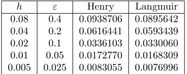
2.4.2. Instantaneous adsorption and local equilibrium We may assume that the process of adsorption of surfactant at the interface is instantaneous, i.e. fast compared to the timescale of convective and diffusive transport. This local equilib-rium corresponds to the case that the bulk chemical potentialG′(c) and the interface chemical potentialγ′(cΓ) are equal, i.e. we set α= 0 in (2.5) (we here only consider one of the bulk phases adjacent to the interface and, for simplicity, drop the upper index (i)). We obtain the following relation (also see [9, 10]):
γ′(cΓ) =G′(c) ⇐⇒ cΓ=g(c) := (γ′)−1(G′(c)), (2.13)
[image:10.612.90.436.98.183.2]where g:R+→R+ is strictly increasing. This function g plays the role of various adsorption isotherms which state the equilibrium relations between the two densities. Table 2.1 displays the functional forms for γ and G in order to obtain the ad-sorption isotherms of Henry, Langmuir, Freundlich, Volmer and Frumkin. The free energies are (variants of) ideal solutions. Here, cΓM is the maximum surfactant den-sity on the interface,K a constant relating the surface density to the bulk density in equilibrium, σ0 denotes the surface tension of a clean interface, B essentially is the sensitivity of the surface tension to surfactant,A in the Frumkin isotherm is known as surface interaction parameter while, in the Freundlich isotherm,Ac measures the
adsorbent capacity andN is the intensity of adsorption.
2.4.3. Insoluble surfactants Neglecting (2.8), (2.12), and the jump term in (2.11) gives a two-phase flow model with insoluble surfactant.
given by the indicator functions on Ω(i) and Γ respectively; see the Appendix for a precise definition. We now define
j1= 1
α(1)(γ
′(cΓ)−G′ 1(c
(1))), j 2=
1
α(2)(γ
′(cΓ)−G′ 2(c
(2))).
In the Appendix we show that
∂t(χΩ(1)c(1)) +∇·(χΩ(1)c(1)v−χΩ(1)Mc(1)∇G′1(c(1))) =δΓj1, (2.14)
∂t(χΩ(2)c(2)) +∇·(χΩ(2)c(1)v−χΩ(2)Mc(2)∇G′2(c(2))) =δΓj2, (2.15)
∂t(δΓcΓ) +∇·(δΓcΓv−MΓδΓ∇γ′(cΓ)) =−δΓ(j1+j2), (2.16)
interpreted in their distributional formulations are equivalent to
∂tc(1)+∇·(c(1)v−Mc(1)∇G′1(c
(1))) = 0, in Ω(1),
Mc(1)∇G′1(c(1))·ν=j1, on Γ,
∂tc(2)+∇·(c(2)v−Mc(2)∇G′2(c
(2))) = 0, in Ω(2),
−Mc(2)∇G′2(c(2))·ν=j2, on Γ,
and (2.11) respectively.
2.6. Non-dimensional evolution equations To derive equations in a di-mensionless form we pick a length scaleL, a time scaleT (or, equivalently, a scale for the velocity V=L/T), a scale Σ for the surface tension, and letCΓ=L−2,C=L−3
denote scales for the surfactant densities in the interface and in the bulk, respectively. The Reynolds number, as the ratio of advective to viscous forces, is defined as Re := (ρ(2)L2)/(η(2)T). The capillary number, as the ratio of viscous to surface tension forces, is defined as Ca = (η(2)L)/(TΣ). Scaling the pressure byT2/(ρ(2)L2) we arrive at the following dimensionless fluid equations:
∇∗·v∗= 0, (2.17)
∂t∗(ρ±v∗) +∇∗·
(
p∗I−2η ±
ReD(v∗) +ρ ±v
∗⊗v∗
)
= 0, (2.18)
[v∗]21= 0, v∗·ν=uΓ∗, (2.19)
[
p∗I−2η ± Re D(v∗)
]2
1
ν= 1
ReCa(σ∗κν+∇Γ∗σ∗), (2.20)
whereη+= 1,η−=η(1)/η(2),ρ+= 1,ρ−=ρ(1)/ρ(2). Let
γ∗=γ
Σ, Gi,∗=
GiL
Σ , M (i)
c,∗=Mc(i)ΣT L
3, M
Γ,∗=MΓΣT L2,
where γ∗,Gi,∗ denote the dimensionless free energies and M
(i)
c,∗,MΓ,∗ denote the
di-mensionless mobilities. The didi-mensionless surfactant equations are given by
∂t•
∗c
(i) ∗ −∇∗·
(
Mc,(i∗)∇∗G′i,∗(c
(i) ∗ )
)
= 0, (2.21)
∂•t
∗c
Γ
∗+cΓ∗∇Γ∗·v∗−∇Γ∗·
(
MΓ,∗∇Γ∗γ∗′(cΓ∗)
)
=
[
Mc,(i∗)∇∗G′i,∗(c
(i) ∗ )
]2
1
ν, (2.22)
α∗(i)(−1)iMc,(i∗)∇∗G′i(c
(i)
∗ )·ν=−(γ∗′(cΓ∗)−G′∗,i(c
(i)
where α(∗i)=α(i)/(TΣL4) is the dimensionless kinetic factor. If we consider the mo-bilities in Section 2.4.1, then we have the relation
Mc,(i∗)=
1 Pec,i
1
G′′i,∗(c(∗i))
, MΓ,∗=
1 PeΓ
1
γ∗′′(cΓ ∗)
,
where Pec,i=L2/(T D
(i)
c ), as the ratio of advection to diffusion of bulk surfactants,
is the bulk Peclet number and PeΓ=L2/(T DΓ) is the corresponding interface Peclet number. The dimensionless surfactant equations with Fickian diffusion read as
∂t•∗c(∗i)−∇∗· (
1 Pec,i∇∗
c(∗i) )
= 0, (2.24)
∂t•
∗c
Γ
∗+cΓ∗∇Γ∗·v∗−∇Γ∗·
(
1 PeΓ
∇Γ∗cΓ∗
)
=
[
1 Pec,i
∇∗c(∗i)
]2
1
ν, (2.25)
α(∗i)(−1)
i
Pec,i ∇∗
c(∗i)·ν=−(γ∗′(c∗Γ)−G′∗,i(c(∗i))). (2.26)
3. Phase field model
3.1. Model for two-phase fluid flow In this section we will derive a phase field model for two-phase flow with surfactant generalizing the work by Abels, Garcke, and Gr¨un on phase field modelling of two-phase flow [1]. We start by recapitulating their essential assumptions and governing equations.
For a test volumeV ⊂Ω, let ρdenote the total mass density of the mixture inV
and, for i= 1,2, denote by ρ(i),V
i the bulk density and the volume occupied by fluid
iin V, respectively. Let ui=Vi/V denote the volume fraction occupied by fluid iin
V. Assuming zero excess volume due to mixing, we have
u1+u2= 1. (3.1)
Then the total density ρcan be expressed as a function of the difference in volume fraction φ=u2−u1, which is a natural choice for the order parameter that distin-guishes the two fluids,
ρ=ρ(φ) =ρ
(2)(1 +φ) 2 +
ρ(1)(1−φ) 2 =
ρ(2)−ρ(1)
2 φ+
ρ(2)+ρ(1)
2 . (3.2)
As in [1, 26], we assume that the inertia and kinetic energy due to the motion of the fluid relative to the gross motion is negligible. Therefore we consider the mixture as a single fluid with velocityv. If one choosesv to be the volume averaged velocity then the prototype diffuse interface model for incompressible two-phase flow with different densities is
∇·v= 0, (3.3)
∂t(ρv) +∇·(ρv⊗v) =∇·T, (3.4)
∂tφ+∇·(φv) =−∇·Jφ, (3.5)
whereT is a tensor yet to be specified,Jφis a flux related to the mass fluxJ by
As a consequence of (3.5) we obtain the mass balance law
∂tρ+∇·(ρv) =−∇·J. (3.7)
Our goal is now to extend this model to the case where surfactants are present, distinguishing the cases of dynamic and instantaneous adsorption. We proceed as in the sharp interface setting by postulating appropriate mass balance equation(s) for the surfactant and deriving models from constitutive assumptions such that thermo-dynamic consistency is guaranteed.
3.2. Dynamic adsorption (Model A)
3.2.1. Mass balance equations We will use the distributional forms for the bulk and interfacial surfactant equations to derive the phase field surfactant equations. Since the sharp interface is replaced by an interfacial layer, we consider regularisations of χΩ(i) and δΓ that appear in (2.14),(2.15),(2.16). In the context of phase field models, many regularisations of the delta function are available from the literature [50, 19, 45], but it will turn out that the Ginzburg–Landau free energy density
ε
2|∇φ| 2
+1
εW(φ)
is a suitable regularisation for a multiple of δΓ, where ε is a measure of interfacial thickness and W(φ) is a potential of double-well or double-obstacle type [8] with equal minima at φ=±1 and symmetric about φ= 0. For example, one can choose
W(φ) =14(1−φ2)2 for a potential of double-well type or
W(φ) =1 2(1−φ
2) +I
[−1,1](φ), I[−1,1](φ) =
{
0, if |φ| ≤1,
∞, else,
for a potential of double-obstacle type. However, in the following derivation we as-sume a smooth potential for convenience. The potential termW(φ) prefers the order parameterφin its minima at±1 and the gradient term |∇φ|2 penalises large jumps in gradient. This leads to the development of regions where φ is close to±1 which are separated by a narrow interfacial layer. We define
δ(φ,∇φ) :=W
( ε
2|∇φ| 2
+1
εW(φ) )
,
where W is a calibration constant that depends on the choice of the potential W, chosen such that δ(φ,∇φ) regularisesδΓ; see [43]. In particular, for the two choices ofW discussed above, we set
1
W=
∫ ∞
−∞
2W(tanh(z/√2))dz= 2√2/3, for the double-well potential,
∫ π/2
−π/2
2W(sin(z))dz=π/2, for the double-obstacle potential. (3.8)
For the regularisation ofχΩ(2), we considerξ2(φ) to be a non-negative cut-off function
such thatξ2(1) = 1,ξ2(−1) = 0 andξ2varies smoothly across|φ|<1. For example, in some of the subsequent numerical experiments we used
ξ2(φ) =
1, φ≥1,
1 2(1 +
1 2φ(3−φ
Similarly,ξ1(φ) = 1−ξ2(φ) will be the regularisation ofχΩ(1).
Our ansatz for the case of dynamic adsorption of the surfactant to the interface is motivated by the distributional formulation in (2.14)-(2.16)
∂t(ξi(φ)c(i)) +∇·(ξi(φ)c(i)v) +∇·(ξi(φ)Jc(i)) =δ(φ,∇φ)ji, i= 1,2, (3.9)
∂t(δ(φ,∇φ)cΓ) +∇·(δ(φ,∇φ)cΓv) +∇·
(
δ(φ,∇φ)JΓ
)
=−δ(φ,∇φ)(j1+j2), (3.10)
where Jc(i) is the bulk surfactant flux, JΓ is the interfacial surfactant flux, and ji,
i= 1,2, denote the mass exchange between the bulk and the interfacial regions. In the above prototype model we allow the situation where there are surfactants present either in both bulk phases or in just one bulk phase. We denote the former as the two-sided model and the latter as the one-sided model. In the one-sided model, we set c(1)≡0, ξ
1(φ)≡0, j1≡0,Jc,1≡0, and we drop the subscripts so that equations (3.9),(3.10) are written as
∂t(ξ(φ)c) +∇·(ξ(φ)cv) +∇·(ξ(φ)Jc) =δ(φ,∇φ)j,
∂t
(
δ(φ,∇φ)cΓ )
+∇·(δ(φ,∇φ)cΓv) +∇·
(
δ(φ,∇φ)JΓ
)
=−δ(φ,∇φ)j.
Observe that, for a test volumeV(t) with external normalν, we have
d dt
( ∑
i=1,2
∫
V(t)
ξic(i)+
∫
V(t)
δcΓ )
=−
∫
∂V(t)
(ξ1Jc(1)+ξ2Jc(2)+δJΓ)·ν,
which is analogous to (2.2).
3.2.2. Energy inequality We introduce a Helmholtz free energy density
a(φ,∇φ,c(i),cΓ) which will play the role of the bulk and interfacial free energy density for the diffuse interface model. As in the sharp interface setting and in analogy to (2.3) the total energy in a test volumeV is the sum of the kinetic and free energy:
∫
V
e(v,φ,∇φ,c(i),cΓ) =
∫
V
ρ|v|
2
2 +
∫
V
a(φ,∇φ,c(i),cΓ), (3.11)
where
a(φ,∇φ,c,cΓ) =δ(φ,∇φ)γ(cΓ) +ξ1(φ)G1(c(1)) +ξ2(φ)G2(c(2)).
Since δ(φ,∇φ) approximatesδΓ we can consider the first term as an approximation of the surface free energy density. We assume that the free energy densities satisfy
γ′′>0,G′′i>0 and that the following dissipation law holds pointwise inV:
−D:=∂te+∇·(ve) +∇·Je≤0, (3.12)
whereJeis an energy flux that we will determine later.
From (3.7) and (3.4) we have
∂t
(
ρ|v|2
2
)
+∇·
(
ρ|v|2
2 v
)
=−|v2|2∇·J+ (∇·T)·v+ [(∇·J)v]·v
=−|v2|2∇·J+ (∇·T)·v+ [∇·(v⊗J)]·v−[(J·∇v)]·v
=∇·
(
−|v|2
2 J+T⊥v
)
−T:∇v+ [∇·(v⊗J)]·v
=∇·
(
−|v|2
2 J+ (T⊥+ [v⊗J]⊥)v
)
We use the identities
∂t•∇φ=∇∂t•φ−(∇v)⊥∇φ, ∂t•(ab) =a∂t•b+b∂•ta,
∂t•(δ(φ,∇φ)γ(cΓ)) =∂t•(δ)γ(cΓ) +γ′(cΓ)∂•t(cΓ)δ
=∂t•(δ)γ(cΓ) +γ′(cΓ)∂t•(δcΓ)−γ′(cΓ)cΓ∂t•(δ), ∂t•(ξi(φ)Gi(c(i))) =∂t•(ξi(φ)c(i))G′i(c
(i)) +∂•
t(ξi(φ))(Gi(c(i))−c(i)G′i(c
(i)))
to obtain after some lengthy calculations that
−D=∇·
(
Je−J|v|
2
2 +T⊥v+ (v⊗J)v
)
+∇·
(
−δγ′(cΓ)JΓ−
∑
i=1,2
ξiG′i(c
(i))J(i)
c +Wεσ∇φ∂•tφ
)
+∇·
(
Jφ
( ∑
i=1,2
ξ′i(φ)(Gi(c(i))−G′i(c
(i))c(i))−∇·(Wεσ∇φ) +W
ε σW
′(φ)))
+δJΓ·∇γ′(cΓ) +ξ1Jc(1)·∇G′1(c(1)) +ξ2Jc(2)·∇G′2(c(2))
−δj1(γ′(cΓ)−G′1(c(1)))−δj2(γ′(cΓ)−G′2(c(2)))
+Jφ·∇
( ∑
i=1,2
ξ′i(φ)(Gi(c(i))−G′i(c(i))c(i))−∇·(Wεσ∇φ) + W
ε σW
′(φ))
−(∇·v)
(
φ( ∑
i=1,2
ξi′(φ)(Gi(c(i))−G′i(c
(i))c(i))−∇·(Wεσ∇φ) +W
ε σW
′(φ)))
+ (∇·v)
(
δσ+ξ1(G1(c(1))−G′1(c
(1))c(1)) +ξ
2(G2(c(2))−G′2(c
(2))c(2)))
−∇v: (T+v⊗J+Wεσ∇φ⊗∇φ).
In the case where the surfactant is present in only one of the bulk phases, a similar calculation shows that we obtain the above form for−Dwithout any terms involving the subscript 1.
In any case, we chooseJeso that the divergence term cancels.
3.2.3. Constitutive assumptions We set
µ=−∇·(Wεσ(cΓ)∇φ)+W
ε σ(c
Γ)W′(φ) + ∑
i=1,2
ξ′i(φ)(Gi(c(i))−G′i(c(i))c(i))
and make the following constitutive assumptions:
JΓ=−MΓ(cΓ)∇γ′(cΓ), Jc(i)=−Mc(i)(c(i))∇G′i(c(i)),
ji=
1
α(i)
(
γ′(cΓ)−Gi′(c(i))),
Jφ=−m(φ)∇µ,
for some non-negative functionm(φ). We choose the tensorT to be
T=
(
σδ+∑
i=1,2
ξi(Gi(c(i))−G′i(c
(i))c(i))−φµ)I
wherepdenotes the unknown pressure,η(φ)>0 denotes the viscosity defined similar to (3.2), interpolating between two bulk viscosities η(1) and η(2). From (3.6) the volume diffuse fluxJ is given by
J=−ρ(2)−2ρ(1)m(φ)∇µ.
Since the interface thickness will be of orderε, it turns out that the term
∇·(σ(δ(φ,∇φ)I−Wε∇φ⊗∇φ))
scales withε−2, while the term
∇·(ξ1(G1(c(1))−G′1(c(1))c(1))I+ξ2(G2(c(2))−G′2(c(2))c(2))I−φµI)
scales with ε−1, the same order as the pressurep. Hence we absorb the latter term as part of the pressure and reuse the variablepas the rescaled pressure, leading to
T=σ(cΓ)(δ(φ,∇φ)I−Wε∇φ⊗∇φ)−pI+ 2η(φ)D(v)−v⊗J.
We remark that the term∇·(σδ(φ,∇φ)I) in the momentum equation is required to recover the surface gradient of the surface tension in the asymptotic analysis. It is present also in other diffuse interface models with Marangoni effects [48, 31, 39].
With the above assumptions we obtain the energy inequality
−D=−m(φ)|∇µ|2−∑
i=1,2
Mc(i)(c(i))ξi(φ)∇G′i(c
(i))2−2η(φ)|D(v)|2
−∑
i=1,2 1
α(i)δ(φ,∇φ)
γ′(cΓ)−G′i(c(i))
2
−MΓ(cΓ)δ(φ,∇φ)∇γ′(cΓ) 2
≤0,
and the diffuse interface model (denoted Model A) for the case of dynamic adsorption reads
∇·v= 0, (3.13)
∂t(ρv) +∇·(ρv⊗v) =∇·
(
−pI+ 2η(φ)D(v) +v⊗ρ(2)−2ρ(1)m(φ)∇µ )
(3.14)
+∇·(σ(cΓ)(δ(φ,∇φ)I−Wε∇φ⊗∇φ)),
∂t•φ=∇·(m(φ)∇µ), (3.15)
µ+∇·(Wεσ(cΓ)∇φ) =W
ε σ(c
Γ)W′(φ) + ∑
i=1,2
ξ′i(φ)(Gi(c(i))−G′i(c(i))c(i)), (3.16)
∂•t(ξi(φ)c(i)) =∇·(Mc(i)(c
(i))ξ
i(φ)∇G′i(c
(i))) (3.17)
+ 1
α(i)δ(φ,∇φ)(γ
′(cΓ)−G′
i(c
(i))), i= 1,2,
∂t•(δ(φ,∇φ)cΓ) =∇·
(
MΓ(cΓ)δ(φ,∇φ)∇γ′(cΓ)
)
(3.18)
−δ(φ,∇φ)∑
i=1,2 1
α(i)(γ
′(cΓ)−G′
i(c
3.3. Instantaneous adsorption, one-sided (Model B) To model instanta-neous adsorption, we assume that the surfactant is insoluble in one phase Ω(1). As in Section 2.4.2 we assume that the bulk surfactant in Ω(2) and the interface surfactant are in local thermodynamical equilibrium. This means that the bulk chemical poten-tialG′2(c(2)) and the interface chemical potentialγ′(cΓ) are equal. Hence we impose the constraint
γ′(cΓ) =G′2(c(2))
in order to replacecΓ. For this purpose, sinceγ′ is strictly monotone (recall thatγis strictly convex) we may set
g(c(2)) = (γ′)−1(G′2(c(2))) =cΓ.
We then consider one surfactant mass balance equation which we obtain by adding (3.9) fori= 2, (3.10), and settingj1= 0,
∂•t(ξ(φ)c+δ(φ,∇φ)g(c)) +∇·(ξ(φ)Jc+δ(φ,∇φ)JΓ) = 0, (3.19)
in place of (3.9) and (3.10) (for convenience, we drop the index 2 ofξ2,c(2),J (2)
c etc.).
The energy of the system is given by
e(v,φ,∇φ,c) =1 2ρ|v|
2
+δ(φ,∇φ)γ(g(c)) +ξ(φ)G(c),
and we set
µ=−∇·(Wεσ(g(c))∇φ) +W
ε σ(g(c))W
′(φ) +ξ′(φ)(G(c)−G′(c)c),
where
σ(g(c)) =γ(g(c))−γ′(g(c))g(c) =γ(g(c))−G′(c)g(c).
Then, a similar computation as in the previous model yields
−D=∇·(Je−J|v|
2
2 + (v⊗J)v−δγ′(g(c))JΓ−ξG′(c)Jc+Wεσ(g(c))∇φ∂•tφ)
+∇·
(
T⊥v+Jφµ
)
+Jφ·∇µ−∇v: (T+v⊗J+Wεσ(g(c))∇φ⊗∇φ)
+δJΓ·∇γ′(g(c)) +ξJc·∇G′(c).
We chooseJe,T,Jφ as in Model A. Furthermore, we assume that
Jc=−M(c)∇G′(c), JΓ=−MΓ(g(c))∇γ′(g(c)) =−MΓ(g(c))∇G′(c).
We then get the energy inequality
The diffuse interface model for this case (denoted Model B) is
∇·v= 0, (3.20)
∂t(ρv) +∇·(ρv⊗v) =∇·
(
−pI+ 2η(φ)D(v) +v⊗ρ(2)−2ρ(1)m(φ)∇µ )
(3.21)
+∇·(σ(g(c))(δ(φ,∇φ)I−Wε∇φ⊗∇φ)),
∂t•φ=∇·(m(φ)∇µ), (3.22)
µ+∇·(Wεσ(g(c))∇φ) =W
ε σ(g(c))W
′(φ) +ξ′(φ)(G(c)−G′(c)c), (3.23)
∂t•(ξ(φ)c+δ(φ,∇φ)g(c)) =∇·(M(c)ξ(φ)∇G′(c)) (3.24) +∇·(MΓ(g(c))δ(φ,∇φ)∇G′(c)).
3.4. Instantaneous adsorption, two-sided (Model C) We now derive an alternative model for instantaneous adsorption that is two-sided. Since we assume local thermodynamical equilibrium, the chemical potentials G′1(c(1)), G′
2(c(2)) and
γ′(cΓ) are equal on the interface. We therefore introduce a chemical potential, denoted byq, and consider this as an unknown field rather than the densities of the surfactants. Since the free energiesGi,γare strictly convex, their derivatives are strictly monotone
and we obtain a one-to-one correspondence between thec(i) andq, i.e.
c(1)= (G′1)−1(q), c(2)= (G′2)−1(q), cΓ= (γ′)−1(q).
We then also may write the surface tension as a function ofq,
˜
σ(q) =σ(cΓ(q)) =γ(cΓ(q))−cΓ(q)q.
Summing (3.9) for i= 1,2 and (3.10) we obtain the conservation of surfactants as follows:
∂t•(ξ1(φ)c(1)(q) +ξ2(φ)c(2)(q) +δ(φ,∇φ)cΓ(q))
=−∇·(ξ1(φ)Jc(1)+ξ2(φ)Jc(2)+δ(φ,∇φ)JΓ
) .
The energy density of the system is given by
e(φ,∇φ,v,q) =1 2ρ|v|
2
+ξ1(φ)G1(c(1)(q)) +ξ2(φ)G2(c(2)(q)) +δ(φ,∇φ)γ(cΓ(q)),
and similar computations as in the previous models yield
−D=∇·(Je−J|v|
2
2 + (v⊗J)v−δqJΓ−ξ1qJ (1)
c −ξ2qJc(2)+Wεσ˜(q)∇φ∂t•φ)
+∇·
(
T⊥v+Jφµ
)
+Jφ·∇µ−∇v: (T+v⊗J+Wε˜σ(q)∇φ⊗∇φ)
+δJΓ·∇q+ξ1(φ)Jc(1)·∇q+ξ2(φ)J
(2)
c ·∇q,
where
µ= ∑
i=1,2
ξ′i(φ)(Gi(c(i)(q))−qc(i)(q))−∇·(Wεσ˜(q)∇φ) +W
ε σ˜(q)W
′(φ).
ChoosingJe,T,Jφas before (but with thec(i)now as functions ofq), and setting