© Medwell Journals, 2019
Solving a Large-Scale Nonlinear System of Monotone Equations by using a
Projection Technique
Nabiha Kahtan Dreeb, Karrar Habeeb Hashim, Mohammed Maad Mahdi,
H.A. Wasi, Hasan Hadi Dwail, Mushtak A.K. Shiker and Hussein Ali Hussein
Department of Mathematics, College for Pure Science, University of Babylon, Hillah, Iraq
Abstract: In this study, we suggest a new projection algorithm for solving nonlinear systems of monotone equations. The projection methods are an efficient family of derivative free methods for solving nonlinear systems of monotone equation that is in each iteration, the current iterate is strictly separated from the solution set of the problem by an appropriate hyperplane that constructs by the new projection algorithm. Then the current iterate is projected onto this hyperplane to determine the new approximation. Under standard assumptions, the global convergence of the proposed algorithm are proved. The numerical experiments indicate the efficiency of the proposed algorithm.
Key words:Nonlinear system of equations, projection method, monotone strategy, global convergence,
experiments, assumptions
INTRODUCTION
The nonlinear systems and their solutions are of great importance in the various sciences which have included different fields and aspects. It is an important part of the sciences of mathematical and physics (since, most physical systems are nonlinear) as well as their importance in engineering, especially, mechanical engineering, electricity, management, economy, population growth, weather and other natural phenomena. The nonlinear systems are studied alongside the linear system because of the possibility of converting nonlinear problems into linear ones from many variables. Consider the following nonlinear system of equations:
(1)
F x 0
where, Fis a continuous and monotone function from Rn to Rn condition of monotony mean:
(2)
F x -F y
T
x-y 0, x, y R nThe solution of nonlinear system equations is one of the problem and difficulties in the mathematical and engineering applications that analyzing it by analytical methods is difficult. Therefore, we can only rely on iterative methods that use the iterative procedure to obtain approximate solutions. The Newton method may be one of the best numerical methods that use the iterative method to solve these systems and it is consider a smooth method to find approximate values of equations.
In recent years, many modifications have been made to the Newton method these suggested methods may be equivalent to (or better than) the Newton method to solve the nonlinear system of equations. The line search method and the trust region method are the most important two methods to solve these systems.
The important idea of the line search method is finding the step length in the specified direction but the trust region method always cares to find a neighborhood of the current step xk, so that, the new iterate falls within the trust region determined by its radius (Amini et al., 2016) also this technique is used to solve unconstrained optimization (Shiker and Sahib, 2018).
Some methods proved ineffective for solving large-scale nonlinear system of equations as Newton method and quasi-Newton methods (Hager and Zhang, 2005; Li, 2017; Hassan and Shiker, 2018) because they need to solve the Jacobian matrix or an approximation of it in each iterative.
This research focuses on solving the system of large-scale non-linear equations by a new projection technique. The simple idea of the projection technique is always interested in separating the present approximation from the result set of the problem (Eq. 1) by appropriate hyperplane that is built in each iterate and then projecting this approximation on the same hyperplane to obtain the new approximation (Koorapetse et al., 2019). Several researchers use conjugate gradient approaches combining with projection techniques for solving (Eq. 1) as well as optimization issues (Dai, 2002).
The first projection approach was suggested by Solodov and Svaiter (1998) and it showed the totally convergent of solving nonlinear problems. In this study, the new algorithm is used to solve the nonlinear systems, we proved its global convergence. Then we compare with two famous methods, SBM method by Yan et al. (2010) and DFPB1 by Ahookhosh et al. (2013), the new algorithm will be more efficient.
The framework: The projection technique is one of the ways that proved to be active in solving nonlinear problems and it is a suitable and applicable way to solve large-scale difficulties these methods use a series of repetitions to arrive to the next iterate:
(3)
k 1 k k k
x = x + d
Where:
αk = A step length dk = The step direction
These processes are called an iterative procedures (Ortega and Rheinboldt, 1970), so, the projection techniques are called iterative methods. The projection approaches are family of derivative free. To define these effective methods, we use the projection operator ΦΩ[.]. Let ΦΩ[.] be a mapping from Rn to Ω where Ω is non-empty closed convex set (Wang et al., 2003):
(4)
x arg min x-z , z
, x Rn
The projection operator has interesting features is non-expansive property:
(5)
x -
y x-y , x, y Rn
As a result produces:
(6)
x -y x-y , x, y
After a series of iterations, in every iteration, the present approximation xk is isolated from the result set of the problem by the hyperplane Hk that is construction by using a line search technique:
(7)
n T
k K k
H = x R /F z x-z = 0
where:
(8)
k k k k
z = x +a d
By Solodov and Svaiter (1998) suggestion, the following iterate xk+1 can be resolute by projection zk onto Hk where:
(9)
n T
K k k k
C = x R /F z x -z 0
The approximation that is best among all result of system (Eq. 1) can be determined by projection xk onto CK but xkóCk. Then the following approximation, xk+1 can be determined by:
k+1 C k k K
x = P x = arg min x-x | x C
So:
(10)
T k k k
k+1 k 2 k
k
F Z X -Z
x = x - F z
F Z
The suggested method, built on the projection free-derivatives method for the system of nonlinear equations, determine a direction dk, a new direction has foreword as:
(11)
kk
k k
-F x if k = 0 d =
- F x + otherwise
Where:
T k k
k T k k+1 k k k 1 k k k
s s
= , s = x -x , y = F x -F x
y s
With:
k 1 k
k 2
k
F x y =
F x
Generally, used the direction dk which satisfies:
(12)
2 T
k k k
F d -C F
(13)
T
K k k
F z x -z >0
where, C is appositive constant (Ahookhosh et al., 2013). By Shiker and Amini (2018), introduced a new line search strategy for separating hyperplane in projection technique, encourage us to take advantages of this line search which needs αk = {βθi: i = 0, 1, 2, ....} satisfies the condition:
(14)
T
k k k k k k k
-F x + d d F z
Algorithm 1 (NBM):
Input: An initial point x0εRn and the parameters θ, λ, g0 (0.2) and βε
(0.1).
Start Set k = 0 F0 = F (x0)
d0 = -F0
While ||FK||>g
Step 1: Compute ||FK||. If ||FK||#g stop
Set αk = β;
Find the minimum index ik0{1, 2, 3, ...} such that
-F(xk+αk dk)Tdk$θλkαk||F(zk)||
where λk = λ/1+||dk||2
While αk = θikαk
Set zk7xk+αkdk
End while
Step 2: If ||F(zk)||#g, stop. Otherwise compute xk+1 by Eq. 10.
Step 3: Compute dk by Eq. 11:
FK+17F (xk+1);
If FkT dk>-g||Fk||2
dk = -Fk
End if k7k+1 End while End
Remark (R1): Shiker and Amini (2018) from stage 3 of
algorithm 1, it is easy to note that the introduced direction satisfy the sufficient descent condition and for any k, FkTdk#-g||Fk||2.
Convergence possessions: In this part, we need some interesting lemmas and assumptions in showing the global convergence of algorithm 1.
Assumption (B1): The result set of (Eq. 1) is nonempty.
Assumption (B2): The mapping F (x) is Lipschitz
continuous on Rn such that there exists a positive constant M, i.e:
n||F x -F y || M||x-y||, x, y R
Assumption (B3): The mapping F (x) is monotone on Rn
such that:
T
nF x -F y x-y 0, x, y R
Lemma (L1): Zarantonello (1971) let the set ΩfRn be nonempty closed convex set and the projection operator ΦΩ(x) be the projection of x onto closed convex set Ω. For any x, y0Rn, the next statements hold:
C œi0Ω, +ΦΩ(x)-x, z-ΦΩ(x),$0
C +ΦΩ(x)-ΦΩ(y), x-y,$0 and the inquality is strict when ΦΩ(x)…ΦΩ(y)
C ||ΦΩ(x)-ΦΩ(y)||#||x-y||
Lemma (L2): Solodov and Svaiter (1998) assume the assumption B1, B2 and B3 hold and the sequence {xk} is generated via. algorithm1. For any x* such that F (x*) = 0 then:
(15)
* 2 * 2 2
k+1 k k+1 k
||x -x || ||x -x || -||x -x ||
And the sequence {xk} is bounded. Moreover, either the sequence {xk} is finite although, the last iterate is a solution of (Eq. 1) or the sequence {xk} is infinite and:
(16)
k k+1 k
lim||x -x || = 0
Proof: Let x*0Rn be any point such that F (x*) = 0 by monotonicity of F+F(y), x*-y,#0. The hyperplane H = {s0Rn/+F(y), s-y, = 0}, separates x
k from x*, it is easy to satisfy that xk+1 is the projection of xk onto the hyperplane H. Sine x* belongs to this hyperplane from properties of the projection operator (Zarantonello, 1971) we get:
* 2 2 * 2 *
k k k+1 k+1 k k+1 k+1 2
k * 2
k+1
||x -x || = ||x -x || +||x -x || +2 x -x ,x -x
F y ,x -y
+||x -x || ||F y ||
Lemma (L3): Solodov and Svaiter (1998) assume that the assumption B1, B2 and B3 holds and the sequences {xk} and {zk} are generated by algorithm 1 then:
(17)
c 2 k
k 2
k k
||F || min ,
M||d || + ||F z ||
Proof: By the line search rule (Eq. 14), if αk…β then k = θ-1α
k does not satisfy (Eq. 14) this mean that:
-1
T -1
k k k k k k k k k
-F x + d d < ||F z || ||F z ||
where, γk = 1/1+||dk||2. By the Lipchitz continuity of F and (Eq. 12) we get:
T T
2 T
k k k k k k k k
2
k k k k k k k k
C||F || -F d = F z -F x d -F z d
||F z -F x || ||d ||+ ||F z || = M||d || + ||F z ||
So:
2 k
k 2
k k
c||F || M||d || + ||F z ||
Theorem (T1): Assume that B2 and B3 hold and the sequence {xk} is generated by algorithm 1 then:
(18)
k k
lim||F || = 0
Proof: From Eq. 10 and Eq. 14 we get:
(19)
T Tk k k k k k
2 k+1 k
k k
2 2
k k k
2 2
k k k
|F z x -z | - F z d
||x -x || =
||F z || ||F z || ||F z ||
= 1+||d || ||F z || 1+||d ||
By lemma 3 from Ahookhosh et al. (2013), the sequence of direction {dk} that generated by algorithm 1 are bounded there is a constant N>0 such that:
(20)
k||F x || N
And result that for all k there exists a constant L>0 such that:
(21)
k
||d || L
By the Lipschitz continuity of F, it can be concluded that:
(22)
k k k k
k k k k
||F z || ||F z -F x ||+||F x || M z -x +N = M ||d ||+N
From (Eq. 19) together with (Eq. 21) gives:
2
2 k
k+1 k 2
||x -x || 1 L So: (23) 2 lim 2 lim k
k||x -x ||k+1 k k 1+L2 limk k||d ||0k
Now by using Cauchy Schwartz inequality along with (Eq. 12), we get:
2 T
k k k k k
C||F || -F d ||F || ||d ||
So:
(24)
k k
||d || C||F ||
For all k. Giving to this condition and (Eq. 23), it follows that:
(25)
k k
lim 0
On the other hand, multiplying (Eq. 17) by ||dk||2 result that:
(26)
2 2
2 2 k
k k k 2
k k
CL ||F || ||d || min ||d || ,
ML + M ||d ||+N
From (24) and (26) we have:
(27)
2 2
0||F ||k k||d ||k Where:
2 2 0 2 k k CL = min c ,ML + M ||d ||+N
The relation (23) and (27) conclude that limk64||Fk|| = 0.
Numerical experiment: In this study, we compare the
performance of the new algorithm (NBM) with tow famous algorithms:
SBM: This technique is taken from Yan et al. (2010) and it uses two modified HS approaches with the projection technique by Solodov and Svaiter (1998).
DFPB1: This technique is taken from Ahookhosh et al. (2013), it uses a three-term PRP-based conjugate gradient direction.
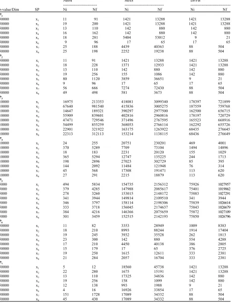
The performances of these approaches are compared with reference to the number of iterations Ni, the number of function evaluations Nf and CPU time. In order to compare these algorithms, some well-known test problems by Ahookhosh et al. (2013) and Yan et al. (2010) are used where the dimensions are confined between 5000-50000 for the taken primary points.
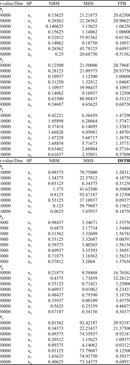
The tests were run on a PC with CPU 2.70 GHz and 4 GB RAM. All of the codes were written in MATLAB R2014 a programming environment. The running of the codes checks if the provided data for problems in all algorithms converges to the equal points. All of the algorithms terminate whenever ||Fk||#10-8 or ||F(zk)||#10-4 or the whole number of iterates surpasses 500000. In all of the algorithms, the parameters are stated as follows θ = 0.4, β = 0.9, λ = 0.1, 0 = 10-8. The numerical results of consecutively the algorithms are registered in Table 1 and 2. Table 1 contains Ni and Nf while Table 2 contains the numerical results of CPU time.
Table 1: Numerical results (Ni and Nf)
NBM MHS DFPB
--- ---
---p-value/Dim SP Ni Nf Ni Nf Ni Nf
P1
50000 x1 11 91 1421 13288 1421 13288
50000 x2 19 200 1421 13288 1421 13288
50000 x3 13 110 142 880 142 880
50000 x4 16 162 142 880 142 880
50000 x5 18 281 5404 53012 9 21
50000 x6 9 96 17 65 17 65
50000 x7 25 188 4439 40363 88 504
50000 x8 25 198 2252 19238 88 504
P2
50000 x1 11 91 1421 13288 1421 13288
50000 x2 18 228 1371 12933 1421 13288
50000 x3 13 110 142 880 142 880
50000 x4 19 256 155 1086 142 880
50000 x5 80 1120 3859 36651 9 21
50000 x6 9 96 17 65 17 65
50000 x7 56 666 7274 72430 88 504
50000 x8 49 498 581 3673 88 504
P3
10000 x1 16975 213353 418081 3099340 178397 721899
10000 x2 67640 981540 415836 3005275 187559 759768
10000 x3 14647 189321 390297 2977500 162500 656715
10000 x4 55909 839601 402816 2960816 178197 720729
10000 x5 47471 729546 371496 2767595 165523 668916
10000 x6 54499 855259 368053 2766114 162292 655726
10000 x7 22901 321922 163175 1263922 68435 276645
10000 x8 22313 312113 153214 1138115 68436 276649
P4
10000 x1 24 255 20751 230201 469 4001
10000 x2 370 5289 7709 73104 1494 14896
10000 x3 18 183 2231 20120 155 1029
10000 x4 365 5294 12747 135225 244 1713
10000 x5 198 2896 27023 302729 85 395
10000 x6 144 2092 11484 121948 76 314
10000 x7 45 568 17308 191471 113 620
10000 x8 27 291 2215 18879 113 620
P5
5000 x1 494 5834 154735 2156312 75926 1027957
5000 x2 379 4285 147988 2085617 75401 1019862
5000 x3 278 3260 153015 2148172 75883 1027291
5000 x4 341 3944 149814 2109510 341 3944
5000 x5 346 3797 158114 2198306 75839 1026614
5000 x6 333 3718 156045 2174637 75843 1026679
5000 x7 384 4216 146366 2075659 75872 1027109
5000 x8 301 3459 152515 2142193 75850 1026796
P6
50000 x1 11 82 3353 28949 1009 8383
50000 x2 18 210 8993 88244 1914 17404
50000 x3 19 245 3932 35528 262 1813
50000 x4 23 300 142 880 554 4288
50000 x5 17 210 4450 40138 386 2805
50000 x6 15 179 17 65 376 2725
50000 x7 19 250 1615 12611 333 2381
50000 x8 21 284 2057 16704 333 2381
P7
50000 x1 5 12 18560 45738 1421 13288
50000 x2 22 280 1675 15191 1421 13288
50000 x3 13 110 17325 34836 142 880
50000 x4 19 256 158 1099 142 880
50000 x5 12 138 993 1988 9 21
50000 x6 4 16 16926 33854 17 65
50000 x7 151 1728 17089 34332 88 504
Table 2: Numerical results (CPU time)
p-value/Dim SP NBM MHS FPB
P1
50000 x1 0.15625 21.21875 20.62500
50000 x2 0.26562 22.26562 20.90625
50000 x3 0.140625 1.15625 1.06250
50000 x4 0.15625 1.14062 1.00000
50000 x5 0.32812 55.01562 0.01562
50000 x6 0.14062 0.18750 0.10937
50000 x7 0.26562 43.78125 0.60937
50000 x8 0.25 20.68750 0.51562
P2
50000 x1 0.12500 21.50000 20.79687
50000 x2 0.28125 21.09375 20.93750
50000 x3 0.10937 1.12500 1.00000
50000 x4 0.31250 1.32812 1.04687
50000 x5 1.10937 39.98437 0.10937
50000 x6 0.14062 0.10937 0.12500
50000 x7 0.62500 80.98437 0.53125
50000 x8 0.54687 4.65625 0.68750
P3
10000 x1 0.42221 6.36439 1.47290
10000 x2 1.95898 6.28664 1.57473
10000 x3 0.37418 6.14095 1.33835
10000 x4 1.66826 6.05081 1.48701
10000 x5 1.47228 5.68717 1.36782
10000 x6 1.68854 5.71673 1.35753
10000 x7 0.63462 2.60884 0.57164
10000 x8 0.61637 2.35051 0.57096
p-value/Dim SP NBM MHS DFPB
P4
10000 x1 0.09375 70.75000 1.20312
10000 x2 1.34375 22.57812 4.18750
10000 x3 0.03125 6.34375 0.31250
10000 x4 1.375 41.62500 0.50000
10000 x5 0.8125 92.67187 0.12500
10000 x6 0.53125 37.10937 0.09375
10000 x7 0.125 58.79687 0.15625
10000 x8 0.0625 5.85937 0.18750
P5
5000 x1 0.98437 3.34671 1.55750
5000 x2 0.6875 3.17734 1.54468
5000 x3 0.51562 3.32609 1.56765
5000 x4 0.53125 3.32687 0.00593
5000 x5 0.59375 3.40265 1.56156
5000 x6 0.60937 3.35593 1.56953
5000 x7 0.71875 3.16562 1.56218
5000 x8 0.57812 3.2864 1.57656
P6
50000 x1 0.21875 0.58468 16.76562
50000 x2 0.4375 1.73859 32.28125
50000 x3 0.53125 0.71421 3.25000
50000 x4 0.60937 0.01062 8.23437
50000 x5 0.48437 0.79390 5.18750
50000 x6 0.35937 0.00109 5.43750
50000 x7 0.5625 0.25359 4.46875
50000 x8 0.67187 0.34156 4.34375
P7
50000 x1 0.01562 92.42187 20.92187
50000 x2 0.34375 22.23437 21.37500
50000 x3 0.09375 74.35937 0.92187
50000 x4 0.20312 1.15625 1.09375
50000 x5 0.09375 4.14062 0.03125
50000 x6 0.03125 73.79687 0.12500
50000 x7 1.65625 74.93750 0.59375
50000 x8 0.40625 73.34375 0.60937
CONCLUSION
The current research suggests a new projection technique for solving a system of large-scale nonlinear monotone equations. The projection-based algorithms belongs to the class of derivative-free function-value based approaches and it does not use any feature function and derivatives. Likewise, this method allows a simple globalization. The global convergence of the suggested algorithm is proved under standard assumptions. The numerical experiments indicated that the suggested algorithm is very efficient.
REFERENCES
Ahookhosh, M., K. Amini and S. Bahrami, 2013. Two derivative-free projection approaches for systems of large-scale nonlinear monotone equations. Numer. Algorithms, 64: 21-42.
Amini, K., M.A. Shiker and M. Kimiaei, 2016. A line search trust-region algorithm with nonmonotone adaptive radius for a system of nonlinear equations. 4OR, 14: 133-152.
Dai, Y.H., 2002. Convergence properties of the BFGS algoritm. SIAM. J. Optim., 13: 693-701.
Hager, W.W and H.C. Zhang, 2005. A new conjugate gradient method with guaranteed descent and efficient line search. SIAM J. Optimizat., 16: 170-192.
Hassan, Z.A.H. and M.A.K. Shiker, 2018. Using of generalized bayes theorem to evaluate the reliability of aircraft systems. J. Eng. Appl. Sci., 13: 10797-10801.
Koorapetse, M., P. Kaelo and E.R. Offen, 2019. A scaled derivative-free projection method for solving nonlinear monotone equations. Bull. Iran. Math. Soc., 45: 755-770.
Li, M., 2017. An liu-storey-type method for solving large-scale nonlinear monotone equations. Numer. Funct. Anal. Optim., 35: 310-322.
Ortega, J.M. and W.C. Rheinboldt, 1970. Iterative Solution of Nonlinear Equations in Several Variables. SIAM, Bangkok, Thailand, ISBN:9780898719468, Pages: 572.
Shiker, M.A. K. and K. Amini, 2018. A new projection-based algorithm for solving a large-scale nonlinear system of monotone equations. Croatian Oper. Res. Rev., 9: 63-73.
Solodov, M.V. and B.F. Svaiter, 1998. A Globally Convergent Inexact Newton Method for Systems of Monotone Equations. In: Reformulation: Nonsmooth, Piecewise Smooth, Semismooth and Smoothing Methods, Fukushima, M. and L. Qi (Eds.). Springer, Boston, Massachusetts, ISBN:978-1-4419-4805-2, pp: 355-369.
Wang, Y.J., N.H. Xiu and J.Z. Zhang, 2003. Modified extragradient method for variational inequalities and verification of solution existence. J. Optim. Theor. Appl., 119: 167-183.
Yan, Q.R., X.Z. Peng and D.H. Li, 2010. A globally convergent derivative-free method for solving large-scale nonlinear monotone equations. J. Computat. Applied Math., 234: 649-657.