A Thesis Submitted for the Degree of PhD at the University of Warwick
Permanent WRAP URL:
http://wrap.warwick.ac.uk/82141
Copyright and reuse:
This thesis is made available online and is protected by original copyright.
Please scroll down to view the document itself.
Please refer to the repository record for this item for information to help you to cite it.
Our policy information is available from the repository home page.
Approximation Algorithms for Packing and
Buffering Problems
by
Nicolaos Matsakis
Thesis
Submitted to the University of Warwick
for the degree of
Doctor of Philosophy
Department of Computer Science
Contents
Acknowledgments iii
Declarations iv
Abstract v
Chapter 1 Introduction 1
1.1 Our Contribution . . . 13
Chapter 2 Online Packing Linear Programs 19
2.1 Introduction . . . 19
2.2 The upper bound for deterministic online algorithms . . . 23
2.3 The upper bound for randomized online algorithms . . . 30
2.4 An optimal online algorithm for linear programs with two variables . 35
2.5 Open Problems . . . 38
Chapter 3 The COLORFUL BIN PACKINGproblem 40
3.1 Introduction . . . 40
3.2 An approximation algorithm for theCOLORFUL BIN PACKINGproblem 48
3.2.1 Preliminaries . . . 48
3.2.2 Analysis . . . 51
Chapter 4 Online Buffer Management 60
4.1 Introduction . . . 60
4.2 TheLQD algorithm . . . 64
4.2.1 Preliminaries . . . 64
4.2.2 Analysis . . . 76
4.2.3 The LQDalgorithm for three-port switches . . . 79
4.2.4 The LQDalgorithm for two-port switches . . . 87
Acknowledgments
First and foremost, I am indebted to Matthias Englert for his guidance as my
supervisor in Warwick. His help into teaching me how to arrange my ideas into
concrete mathematical proofs has been crucial.
I am, also, indebted to my current advisors Artur Czumaj and Ranko Lazi´c
and to my former advisor Maxim Sviridenko, for helping me to improve my research
potential. I would, also, like to thank my collaborator Marcin Mucha for discussing
with me some of the ideas I had on various research problems.
Finally, I was very fortunate to have made very good friends, during the
years that I have spent in Warwick. I would like to thank Ebrahim, Lehilton,
Luk´aˇs, Matthew, Michail and Raphael for all the good times we had and I wish to
Declarations
None of the work presented in this thesis has been submitted for a previous degree at
any university. All work was conducted during my period of study in the University
of Warwick.
Chapter 2 is based on joint work with Matthias Englert and Marcin Mucha
(Englert et al. [2014]), which was published in the proceedings of the 11th Latin
American Theoretical Informatics Symposium (LATIN 2014), held in Montevideo,
Uruguay, between March 31 and April 4 2014.
Chapter 3 is based on joint work with Matthias Englert.
Chapter 4 includes individual work (Matsakis [2016], to appear) which has
been accepted for publication by the Student Research Forum of the 42nd
Interna-tional Conference on Current Trends in Theory and Practice of Computer Science
Abstract
This thesis studies online and offline approximation algorithms for packing and buffering problems.
In the second chapter of this thesis, we study the problem of packing linear programs online. In this problem, the online algorithm may only increase the values of the variables of the linear program and his goal is to maximize the value of the objective function of it. The online algorithm has initially full knowledge of all parameters of the linear program, except for the right-hand sides of the constraints which are gradually revealed to him by the adversary. This online problem has been introduced by Ochel et al. [2012]. Our contribution (Englert et al. [2014]) is to provide improved upper bounds for the competitiveness of both deterministic and randomized online algorithms for this problem, as well as an optimal deterministic online algorithm for the special case of linear programs involving two variables.
In the third chapter we study the offline COLORFUL BIN PACKING prob-lem. This problem is a variant of the BIN PACKING problem, where each item is associated with a color and where there exists the additional restriction that two items packed consecutively into the same bin cannot share the same color. The COLORFUL BIN PACKING problem has been studied mainly from an online per-spective and has been introduced as a generalization of the BLACK AND WHITE BIN PACKING problem (Balogh et al. [2012]), i.e., the special case of this prob-lem for two colors. We provide (joint work with Matthias Englert) a 2-appoximate algorithm for the COLORFUL BIN PACKING problem.
In the fourth chapter we study the Longest Queue Drop (LQD) online algo-rithm for shared-memory switches with three and two output ports. The Longest Queue Drop algorithm is a well-known online algorithm used to direct the packet flow of shared-memory switches. According to LQD, when the buffer of the switch becomes full, a packet is preempted from the longest queue in the buffer to free buffer space for the newly arriving packet which is accepted. We show (Matsakis [2016], to appear) that the Longest Queue Drop algorithm is (3/2)-competitive for three-port switches, improving the previously best upper bound of 5/3 (Kobayashi et al. [2007]). Additionally, we show that this algorithm is exactly (4/3)-competitive for two-port switches, correcting a previously published result claiming a tight upper bound of 4M−4
3M−2 <4/3, whereM ∈Z
Chapter 1
Introduction
This thesis deals with several problems in the areas of online and offline computation.
Let us start by providing the informal definition of one of the problems considered
in this thesis: Assume that we are given a set of rectangular items, each of which has
a unit width and a height which is at most one. Suppose, also, that we are supplied
with an unlimited number of square bins of unit dimensions. We are asking what is
the minimum number of bins used, so that each item is packed into a bin and the
sum of the sizes of the packed items into each bin is at most one.
This problem is called BIN PACKING and its various settings have a wide
range of practical applications from the design of integrated circuits to the backup
file storage and the cargo shipping in the transport industry. Hence, it should
come as no surprise that BIN PACKING is one of the most well-studied problems
in the area of theoretical computer science, with relevant publications ranging over
a period of several decades (Ullman [1971]; Johnson [1973]; Karmarkar and Karp
[1982]; Simchi-Levi [1994]; Rothvoß [2013]; D´osa and Sgall [2013]).
Assuming that the conjectureP 6=N P is true, as most of the researchers in
the area believe, it is not possible to derive an algorithm which will run in polynomial
time in the size of the input to this problem, for any input toBIN PACKING,
exponential-time algorithms may require prohibitive running times even for
practi-cal input instances of every-day use, we need to look towards obtaining algorithms
that will run in polynomial time in the size of the input (or to be computationally
efficient algorithms, as we shall say) to BIN PACKING, relaxing our requirement of solving this problem exactly to solving it approximately, but within a reasonable
amount of time.
We emphasize on the fact, however, that any algorithm for BIN PACKING
is assumed to have complete information on the input instance of this problem a
priori, that is the sizes of all given items are known in advance and this information
can be used during the computation.
Let us, now, proceed towards giving a second example of a problem: Suppose
that tasks arrive one by one over time and each of them has to be assigned upon its
arrival to a processor, from a finite set of parallel processors of, possibly, different
processing speeds. The processing of the assigned tasks starts when the last arriving
task has been assigned to a processor and each task assignment is irrevocable, which
means each task has to be processed by the processor that it has been initially
assigned to. Unfortunately, we are provided with no information regarding the
processing time requirement of any task until this task arrives and we are unaware
of the number of remaining tasks to arrive until the last task arrives. Our objective
is to assign each task to a processor such that the time it takes until all processors
end their processing is minimized. This problem is one of the many variants of
LOAD BALANCING. The various settings of LOAD BALANCING have been, also,
extensively studied in the relevant literature (Graham [1969]; Azar et al. [1994];
Bartal et al. [1995]; Azar et al. [1995]; Albers [1999]).
In the case ofLOAD BALANCINGwe are provided with incomplete knowledge
on the input of the problem. An algorithm for this problem has no information
regarding the processing time requirement of any task and the number of remaining
given unlimited computational resources (contrary to our first example of the BIN
PACKING problem), an algorithm for LOAD BALANCING is restricted to perform
under a state of uncertainty regarding the sequence of arriving tasks.
It is, also, worth mentioning that since each task assignment is irrevocable,
the decision of an algorithm to assign any task to a processor, may have an
irre-versible impact on its overall performance. In other words, the task assignment that
an algorithm forLOAD BALANCINGoutputs, may not be one of those assignments
which minimize the time it takes for all processors to complete their processing,
for a given input of arriving tasks. We note that this may be the case even if the
given input sequence is comprised by relatively few tasks and, therefore, for an input
where a reasonable amount of time for the completion of the computation is not an
issue of concern.
The aforementioned computational efficiency and the lack of information
regarding the input instance of the problem are not the only restrictions that an
algorithm may be imposed with. We may recall, here, the space storage requirements
that an algorithm may be, also, imposed with. In this thesis, however, we shall only
deal with algorithms that are restricted to complete in time which is upper-bounded
by a polynomial in the size of the input to the given problem or algorithms that are
restricted to perform under a state of incomplete information regarding the input
instance.
The two described problems,BIN PACKINGandLOAD BALANCING, are two
examples of optimization problems. An optimization problem can be either a cost
minimization problem or a profit maximization problem.
For each inputI to a minimization problemP (belonging to a setI of legal
inputs toP), there exists a set of feasible outputs F(I) and for each feasible output
O∈F(I) there exists a positive real numberg(I, O), which is thecost. The function
for this given input. Finally, anoptimal algorithm forP is an algorithm which for any inputI ∈ I outputs an optimal solution.
In a similar way, but for the case of a maximization problemP0, there exists
an objective function (or profit function) that associates each legal input to the problemP0 and the derived output, with a positive real number, which is the profit.
The optimal solution to an input instance of P0 is a feasible output achieving the
largest value of the objective function, for the given input. Finally, an optimal
algorithm forP0 is an algorithm which for any legal input to this problem, outputs
an optimal solution.
An optimization problem, where the information on the input instance is
gradually received by the algorithm and the output of the algorithm has to be
produced in an online manner, is called online problem. This lack of information refers solely to the input instance and not to the parameters of the problem. For
example, in the case of the previously described variant of LOAD BALANCING,
the number of parallel processors and the processing speed of each of those are
considered to be parameters that are known in advance.
Even though the running times of algorithms are generally considered to be
an irrelevant issue for the area of online computation, we prefer obtaining online
algorithms (as we shall call the algorithms solving online problems) that are
compu-tationally efficient. In fact, it is quite interesting to mention that the great majority
of published online algorithms in the relevant literature happen to be
computation-ally efficient as well (Borodin and El-Yaniv [1998]; Fiat and Woeginger [1998]).
On the other hand, if complete information on the input is provided to the
algorithm a priori, then the optimization problem is called offline and this algo-rithm is calledoffline, as well. The analysis of offline approximation algorithms for NP-hard optimization problems deals with the subject of deriving computationally
efficient algorithms which will guarantee to produce solutions of a satisfactory
that will be considered preferable from exact algorithms that run in exponential
time in the size of the input to this problem.
Whilst some optimization problems can be viewed as being naturally offline
and others as having an online character, there exists a large number of problems
that have been studied from both an online and an offline aspect, due to their rich
variety of practical applications from both of these perspectives. For instance, the
offlineBIN PACKINGproblem has been extensively studied in the relevant literature,
as we have already mentioned. However, the onlineBIN PACKINGproblem has been,
also, studied to a great extent (Lee and Lee [1985]; Ramanan et al. [1989]; Seiden
[2002]; Balogh et al. [2015c]) as we shall see in Chapter 3.
Let us, now, concentrate solely on offline computation, for a while. The
study of offline approximation algorithms for NP-hard optimization problems started
to flourish around the early 1970’s, after the breakthrough papers of Cook [1971]
and Karp [1972] were published. However, approximation algorithms for NP-hard
problems had been derived before even the concept of NP-hardness was introduced;
we may recall here an approximation algorithm for theMINIMUM EDGE COLORING
problem which is due to Vizing [1964].
An immediate question that may arise is how two offline approximation
algo-rithms for the same NP-hard optimization problem are compared to each other, or
to rephrase this, how the quality of the offline approximation is being quantified. We
shall only deal with deterministic offline algorithms here without having to mention
this explicitly.
Hence, letting OPT denote an optimal algorithm for a cost minimization
offline problemP and assuming thatALG(I) denotes the cost of any algorithmALG
when provided with an inputI ∈ I forP, we have the next definition.
Definition 1.1. The approximation ratio of an offline algorithm A forP is defined as RA = supI{
A(I)
OPT(I)}, where I ranges over all legal inputs toP.
because no algorithm may give a cost function value smaller than the optimal one,
for the same input. Finally, we say that the offline algorithmAisα-approximate, if
it holdsα≥RA for an α≥1.
In the case of a profit maximization offline problem P0, we similarly obtain
the next definition, where we assume thatALG(I) denotes the profit of any algorithm
ALGwhen provided with a legal input I forP0 and OPT an optimal algorithm for
the same problem:
Definition 1.2. The approximation ratio of an offline algorithm Bfor P0 is defined
as R0B = infI{OPTB(I()I)}, where I ranges over all legal inputs to P0.
It holds 0< R0B ≤1 since the profit was defined as a positive real number and
because no algorithm may provide a profit function value greater than the optimal
one, for the same input. Finally, we say that Bis a β-approximate algorithm, if it
holdsβ ≤R0B for a positive β.
It is, sometimes, the case to study the performance of an approximation
algorithm for a cost minimization problem, solely for inputs for which the optimal
cost is very large. For this, we define theasymptoticapproximation ratio. Therefore, denoting as OPT(I) the optimal cost for a legal input I to a cost minimization
problem P and as A(I) the cost of an offline algorithm A for the same input, we
have the next definition:
Definition 1.3. The asymptotic approximation ratio of Afor the cost minimization problem P is defined as R∞
A = lim sup
n→∞ supI{
A(I)
OPT(I)|OPT(I) = n}, where I ranges over the set of all legal inputs to P.
The analysis of the performance of any algorithm, whether this is offline or
online, can be categorized as being average-case analysis or worst-case analysis. The
approximation ratio was just defined in terms of the latter approach, as it may be
Especially for the case of online computation, on which we shall concentrate
from now and until the end of this brief introduction, the worst-case analysis studies
the performance of the examined online algorithm towards the performance of an
optimal algorithm which is provided with the advantage of having complete
infor-mation of the input, in advance. Note that such an optimal offline algorithm, as we
shall simply refer to it from now, may not be a realizable algorithm, since complete
information about the input instance is usually an unrealistic scenario for practical
applications of online problems.
On the other hand, the average-case analysis works by first assuming a
dis-tribution of inputs to the examined online problem and then, based on this input
distribution, the expected performance of the online algorithm is obtained.
A disadvantage of the worst-case analysis is that the comparison with an
optimal offline algorithm which is provided with a power that may be unrealistic
could underestimate the performance of the online algorithm. On the other hand, an
undisputable disadvantage of the average-case analysis is the difficulty in obtaining
an input distribution representative of the one that the online algorithm is actually
faced with. Obviously, a non-representative input distribution may lead to an
er-roneous estimation of the actual algorithmic performance, an issue which is easily
bypassed by the worst-case analysis, which makes no probabilistic assumptions on
the input.
It is not in our scope to further discuss on the advantages and disadvantages
of these two approaches. We shall only emphasize on the fact that it is the worst-case
analysis that has become the predominant approach of examining the performance
of online algorithms and it is known as competitive analysis (Karlin et al. [1988]); however, the study of online algorithms in the framework of competitive analysis
had already been initiated several years before the influential publication of Karlin
et al. [1988].
to be the paper of Graham [1969], dealing with a simple greedy algorithm for the
LOAD BALANCING problem, when all processors are assumed to have the same
processing speed. The competitive analysis started to evolve significantly during
the 1980’s after the publication of the seminal paper of Yao [1980] about the online
BIN PACKING problem and, especially, after the publication of Sleator and Tarjan
[1985] about two of the most important online problems, thePAGINGand the LIST
UPDATE problem. Borodin and El-Yaniv [1998] and Fiat and Woeginger [1998]
provide excellent surveys regarding the evolution of the competitive analysis.
A question that, again, naturally arises is how the quality of an online
algo-rithmONLis measured in terms of the competitive analysis. For this, letcostALG(I)
denote the cost of any algorithm ALG for a cost minimization online problem P,
when provided with a legal inputI and letOPTdenote an optimal offline algorithm
forP. Then, we have the next definition.
Definition 1.4. The competitive ratio of ONL is defined as inf{c|costONL(I) ≤
c·costOPT(I)}, for all legal inputs I to P.
It holds c ≥ 1, since the cost was defined as a positive real number and
because no algorithm may give an objective function value smaller than the one
that an optimal offline algorithm outputs, for the same input. We say that the
online algorithmONLis ˆc-competitive for a ˆc≥1, if the competitive ratio ofONL is
equal to c ≤ ˆc. If ˆc = c, we say that ONL is an exactly c-competitive algorithm. Finally, if the infimum in the above definition is infinity, we shall say thatONL is a
non-competitive algorithm.
In the case of a profit maximization online problem P0, we can similarly
denote as prof itALG(I) the profit of any algorithm ALG for this problem, when
provided with a legal inputI and asOPTan optimal offline algorithm forP0. Then,
we have the next definition.
tosup{p|prof itONL0(I)≥p·prof itOPT(I)}, for all legal inputsI toP0.
It holds 0 < p ≤ 1, since the profit was defined as a positive real number
and because no algorithm may give a profit function value, greater than the one
that an optimal offline algorithm outputs for the same input. In a similar way
as for the case of a cost minimization problem, we say that the online algorithm
ONL0 is ˆp-competitive for a positive ˆp≤1 if the competitive ratio ofONL0 is equal to
p≥pˆ. If ˆp=p, then we shall say thatONL0 is an exactly p-competitive algorithm. Finally, if the supremum in the above definition is 0, we shall say that ONL0 is a
non-competitive algorithm.
We shall only employ competitive analysis on any result related to online
computation, throughout this thesis.
For the cases of those online problems where we want to study the
perfor-mance of an online algorithm for a cost minimization problem, only for inputs for
which the optimal cost is very large, we have the definition of theasymptotic com-petitive ratio. Hence, assuming thatP is a cost minimization online problem, that
OPTdenotes an optimal offline algorithm for this problem and ALG(I) the cost of
any algorithmALGfor an input I, we have the following definition:
Definition 1.6. The asymptotic competitive ratio of an online algorithm ONL for P is defined as CONL∞ = lim sup
n→∞ supI{
ONL(I)
OPT(I)|OPT(I) =n}, where I ranges over all legal inputs toP.
We may refer to the competitive ratio as established in Definition 1.4, as
absolutecompetitive ratio, in order to distinguish it from the asymptotic competitive ratio.
It is worth mentioning that an idea of time progression is inherent in the
online problems. To make this more perceivable, a sequence of requests is made
by the adversary which have to be answered (served) one at a time by the online
adversary continues in a repetitive manner until the last request has been served
and the online computation completes.
In the case of deterministic online algorithms, this usually leads us in
visu-alizing the online problem as a game between an online player and an adversary who has the power of generating the input sequence. The online player, who is
provided with no information on the remaining part of the input at any point in
time, runs the online algorithm and outputs a partial solution. The adversary who
controls the remaining part of the input, modifies it in such a way that the overall
ratio of the performance of the online algorithm to the performance of the optimal
offline algorithm, deteriorates for the side of the online player. Fairly enough, the
adversary is usually referred to asmalicious in the literature of online computation (Borodin and El-Yaniv [1998]; Fiat and Woeginger [1998]).
In the case of randomized online algorithms and in order to make a similar
discussion to that of the previous paragraph, we have to first define what kind of
information the adversary is given about the online algorithm. For this, we shall
distinguish between the following two different types of adversaries (Raghavan and
Snir [1989]; Ben-David et al. [1990]).
The first type of adversary fixes the request sequence based on the description
of the online algorithm. However, the sequence has to be fixed before the online
algorithm starts its computation. It follows that this model of adversary has no
information on any of the random choices made by the online algorithm. This
model of adversary is calledoblivious.
For this, let P denote a cost minimization online problem and OPT(σ) be
the cost of an optimal offline algorithm serving an input sequenceσ for P. Then,
assuming thatRALGis a randomized online algorithm for P, distributed over a set
{ALGy} of deterministic online algorithms forP, we obtain the next definition.
toP, where γ is an additive constant independent of the input.
We note that EY[ALGy(σ)] in Definition 1.7, denotes the expectation with
respect to the distributionY, over the set of deterministic online algorithms{ALGy}
which defines the randomized online algorithmRALG. Finally, since the online
prob-lemP is a cost minimization problem, we have c≥1, by the same reasoning as the
one which follows Definition 1.4.
Definition 1.7 can be easily modified to hold for the case of a profit
maxi-mization online problem P0. More specifically, assuming that OPT(σ) denotes the
profit of an optimal offline algorithm serving the input sequenceσ forP0, we have
the following definition.
Definition 1.8. The randomized online algorithm RALG0 (distributed over a set {ALGx} of deterministic online algorithms forP0) isp-competitive against an
obliv-ious adversary, if EX[ALGx(σ)] +δ ≥ p·OPT(σ) for any input sequence σ to P0,
where δ is an additive constant independent of the input.
By the same reasoning as the one which follows Definition 1.5, it holds that
0< p≤1. We note that EX[ALGx(σ)] denotes the expectation with respect to the
distributionX, over the set of deterministic online algorithms{ALGx} that defines
the randomized online algorithmRALG0.
The second type of adversary that is considered in the relevant literature, is
calledadaptive. Though we shall not deal with adaptive adversaries in this thesis, we proceed towards defining this model of adversary, for consistency.
We distinguish between two types of adaptive adversaries, theadaptive-online and theadaptive-offline adversary.
The adaptive-online adversary is aware of the random choices made so far by
the online algorithm, at any point in time. Based on this information, the
adaptive-online adversary serves immediately the current request and modifies the remaining
adaptive-online adversary has the same power as the oblivious adversary since the
behaviour of the deterministic algorithm is known in advance (Ben-David et al.
[1990]).
The adaptive-offline adversary, also, modifies the remaining part of the
se-quence based on the random choices made so far by the online algorithm but serves
it optimally when the online algorithm has completed its computation. It follows
that an adaptive-offline adversary is aware of any random choice made by the online
algorithm, contrary to the case of the adaptive-online adversary.
The cost (or profit, respectively) of an adaptive adversary for serving a
se-quence of requests is a random variable, since an adaptive adversary is aware of
random choices made by the online algorithm during its computation. This is an
important difference compared to the case of an oblivious adversary, who has to fix
the sequence in advance having no knowledge on any of the random choices made
by the online algorithm.
This complete lack of information regarding any random choice made by
the online algorithm is a source of weakness for an oblivious adversary. To state
this in a different way, randomization can be exploited to a greater extent by the
online player, when he plays against an oblivious adversary rather than against
an adaptive-online adversary. On the other side, the adaptive-offline adversary
is certainly stronger than the adaptive-online adversary; in fact, it can be shown
that randomization cannot be used against an adaptive-offline adversary (Ben-David
et al. [1990]).
Concluding, there exist online problems for which randomized online
algo-rithms against oblivious adversaries perform better in expectation, compared to the
optimal deterministic online algorithms that we have for these problems. TheLIST
UPDATEproblem, to which we referred to before, is one of these problems (Albers
1.1
Our Contribution
Before describing the results obtained in this thesis, we need to state some
defini-tions.
A linear program is an optimization problem which asks for either the
maxi-mization or the minimaxi-mization of an objective function ofd∈Z+variables, subject to
a set of inequalities or equalities, which are calledconstraints. The objective func-tion and all constraints have to be linear funcfunc-tions of the givendvariables. Since any
equality constraint can be substituted by inequality constraints, we usually assume
that all constraints of the linear program are inequalities.
A maximization linear program of d variables has the following standard
form:
max b0x0+. . .+bd−1xd−1
subject to A
x0 .. .
xd−1 ≤ c0 .. .
cm−1
x0, . . . , xd−1 ≥0
All components of the vectors b = (b0,. . ., bd−1) and c = (c0,. . ., cm−1), as well as all entries of the matrixAare assumed to be real numbers. A minimization
linear program has an analogous standard form, where the first m inequalities are
reversed and the objective is the minimization of the given linear function.
In case all components of the vectorsbandcas well as all entries of the matrix
Aare non-negative, then the maximization linear program is called aspacking linear program and the minimization linear program is called ascovering linear program. Apart from this and most importantly, there exists a systematic way to obtain a
linear program, where the newly obtained linear program is called as dual linear program and the initial linear program is called asprimal linear program.
Any solution of a linear program which does not violate a constraint, is called
feasible solution. Thefeasible region is the set of all feasible solutions. The optimal solution of the linear program is a point in the feasible region for which the value of
the objective function is maximized or minimized, depending on whether the linear
program is a maximization or, respectively, a minimization linear program. Finally,
a linear program isinfeasible if it has no feasible solution, that is the feasible region is empty.
Many NP-hard optimization problems can be formulated as integer linear
programs, that is linear programs with the additional constraint that variables may
take only integer values. As a consequence, many offline approximation algorithms
are based on linear programming, since even though solving an integer linear
pro-gram is, in general, an NP-hard problem, solving a linear propro-gram admits
computa-tionally efficient exact algorithms. Hence, taking the relaxation of an integer linear
program where the aforementioned restriction on the variable values is dropped,
can be used in obtaining computationally efficient approximation algorithms for a
great number of NP-hard optimization problems. For this, the primal-dual schema
that we previously referred to is widely used, due to some very useful properties
which hold for the feasible solutions of the dual linear program (Vazirani [2001];
Williamson and Shmoys [2011]).
Apart from this, quite recently there has been observed a research interest
into solving linear programs in an online manner, as well (Buchbinder and Naor
[2009b]). This was mainly in order to facilitate the development of improved online
algorithms for some central online programs, such as one of the most well-studied
and important problems in the area of online computation, the k-server problem
(Bansal et al. [2010, 2011]).
the problem that we describe in the following two paragraphs.
First of all, we suppose that we have a packing linear program in the standard
form that was described before. We assume that the vectorband all entries ofAare
initially revealed to the online algorithm by the adversary. However, the adversary
gradually reveals the components of the vector c to the online player, i.e., at any
point in timet a vector `t is revealed to the online player for which it has to hold
`t ≤ c component wise. The vector `t may be viewed as the current right-hand
side values of the linear program. The online player responds at the current point
in time, by increasing the values of variables of his choice whilst ensuring that a
feasible solution is maintained. The goal of the online player is to maximize the
value of the objective function, when no variable value can be further increased.
A parameter α >1, which is initially revealed to the online player, plays a
central role in this online problem, since the adversary is required to ensure at any
point in timetthat it holds (c−Ax)≤α·(`t−Ax), wherexis the vector denoting
the current online solution.
This problem is introduced by Ochel et al. [2012] as an application of lifetime
optimization in wireless sensor networks. As we shall see, the right-hand sides of
the constraints of the packing linear program may be viewed as lifetimes of batteries
that power sensors in wireless networks. Assuming that we can only estimate each
remaining battery lifetime within some fixed α > 1 approximation of its actual
remaining lifetime, the objective of an online algorithm is to choose amongst a set
of broadcasting scenarios, so that the number of sensor broadcasts is maximized,
until the point in time when the first battery becomes exhausted.
Ochel et al. give a Θ(lnα
α )-competitive deterministic algorithm for this online
problem and prove that the competitive ratio of any deterministic or randomized
online algorithm for it, isO(√1
α).
We improve the upper bound on the competitive ratio of any online
algo-rithm, whether deterministic or randomized, for this problem, toO(ln2α
provide an optimal deterministic Θ(√1
α)-competitive online algorithm for linear
pro-grams that involve two variables.
In Chapter 3 we turn our attention to another packing problem. More
specif-ically, we study a variant of the offlineBIN PACKINGproblem which is called
COL-ORFUL BIN PACKINGproblem. Recall from our previous discussion on this problem,
that the offlineBIN PACKING problem has been extensively studied in the relevant
literature; one of the reasons is that many of its different settings have a number of
practical applications.
Hence, in the COLORFUL BIN PACKING problem each item is additionally
associated with a color and two items packed consecutively into the same bin cannot
share the same color. This problem was introduced by Balogh et al. [2012] for
the special case of two colors, called BLACK AND WHITE BIN PACKING problem.
The COLORFUL BIN PACKING problem has been mainly studied from an online
perspective (D´osa and Epstein [2014]; B¨ohm et al. [2014]; Balogh et al. [2015b]).
A motivating application of theBLACK AND WHITE BIN PACKINGproblem
is the optimized distribution of advertisement breaks in television or radio station
programs (Balogh et al. [2012]). To see that, note that the bins may be viewed as
the program blocks (these usually correspond to one-hour intervals, for the case of
radio station programs), the white items correspond to the advertisement breaks
and the black items correspond to the actual broadcasted program. The goal is to
assign advertisement breaks into the program minimizing the program blocks used.
We provide a 2-approximate algorithm for the offlineCOLORFUL BIN
PACK-ING problem, which runs in time O(nlogn), wheren ∈Z+ denotes the number of
items of the input.
This thesis concludes with the study of an online buffering problem. First of
all, it should be acknowledged that the area of packet transmission management is
of transmission requests that is observed in networks, giving the related problems
an inherently online character. More specifically, due to the high volume of packet
transmissions, some packets have to be discarded; hence, the objective of an online
algorithm has to be the minimization of the number of lost packets when the
in-formation given in advance regarding the remaining sequence of arriving packets is
incomplete.
Therefore, in Chapter 4 we study the Longest Queue Drop (LQD) online
algorithm for memory switches with three and two output ports. A
shared-memory switch is a device equipped with a buffer and a number of input and output
ports. The switches are widely used in directing the packet flow of various networks
and the Longest Queue Drop algorithm is a well-known online algorithm used in
directing the packet flow of switches (Aiello et al. [2008]).
Each arriving packet to the switch is destined to a single output port of it
and can be either accepted or be irreversibly rejected by the switch, upon its arrival
time. Assuming that time is divided into time steps, one packet is transmitted by
each output port of the switch to which at least one packet stored in the buffer is
destined, at the current time step.
According to the Longest Queue Drop online algorithm, any arriving packet
is accepted by the buffer if there exists free buffer space at the time step of its arrival.
On the contrary, if the buffer is full at the time step when the packet arrives, a packet
destined to the output port to which the most packets currently stored in the buffer
are destined, is irrevocably rejected from the switch (or it ispreempted, as we shall say). The preempted packet releases buffer space for the arriving packet, which is
immediately accepted by the buffer. After all packet acceptances and preemptions
take place, at each time step, one packet is forwarded from the buffer to its destined
output port, so that it is transmitted.
We show thatLQDis 1.5-competitive for shared-memory switches equipped
(Kobayashi et al. [2007]) of 5/3, for three-port switches. We, also, show a tight
upper bound of 4/3 for the competitive ratio of LQD for shared-memory switches
equipped with two output ports. This corrects upon a previously published result
Chapter 2
Online Packing Linear Programs
2.1
Introduction
During the recent years there has been observed an interest into solving linear
pro-grams in an online manner. Without doubt, the influential paper of Buchbinder and
Naor [2009a] has been the most important work in this area. In this publication,
Buchbinder and Naor study a range of online problems via a primal-dual schema
that they introduce. Their techniques have triggered applications on subsequent
papers, dealing with a variety of central online problems, including one of the most
important problems in the field of online computation, thek-server problem (Bansal
et al. [2011]).
Let us proceed towards describing briefly one of the online problems that
have been studied by Buchbinder and Naor [2009a]. The introduced primal-dual
schema along with some of its applications on various online problems, is described
in detail by its authors in Buchbinder and Naor [2009b].
Buchbinder and Naor assume that incomplete information about the
max b0x0+. . .+bd−1xd−1
subject to A
x0 .. .
xd−1 ≤ c0 .. .
cm−1
x0, . . . , xd−1 ≥0
More specifically, all components of the vectorcare assumed to be initially revealed
to the online player by the adversary but the components of the vector b and the
entries of the matrixA are gradually revealed to the online player in the following
way: The adversary reveals all coefficients of a variable xj at a time of his choice,
i.e., assuming that time is divided into rounds, at roundj the coefficientbj and the
j-th column of the matrix A are revealed to the online player.
On the other side, the online player may increase the value of any variable
at any point in time but never decrease the value of any variable, ensuring that a
feasible online solution is always maintained. The goal of the online player is to
maximize the value of the objective functionbTx.
We focus on a related online problem which has been introduced by Ochel
et al. [2012]. The linear program is the packing linear program which has the
standard form described above.
We assume that the components of the vectorband the entries of the matrix
A (which we shall call as constraint matrix from now) are initially revealed to the online player, but the components of the vector c (which we shall call as capacity vector) are gradually revealed to the online player by the adversary, in a way that we describe in the next paragraph.
Time is assumed to be discrete. At timetthe adversary reveals to the online
sides of the constraints of the linear program. On the other side, the online player
responds att, by increasing the values of variables of his choice. The online player
may never decrease any variable value and has to additionally ensure that each of
the constraints of the linear program is satisfied, i.e., that a feasible online solution
is always maintained. The goal of the online player remains the same as in the
model of Buchbinder and Naor, that is the maximization of the objective function
value.
Finally, the adversary ensures that the following two conditions hold:
• Each component of the revealed vector`t lower-bounds the respective
compo-nent of the capacity vectorc= (c0, ..., cm−1) and
• Assuming thatxis the current online solution, it holds (c−Ax)≤α·(`t−Ax)
whereα >1 is a parameter which is initially revealed to the online player.
We shall denote asrevealed remaining slack attthe quantity (`t−Ax) and
astrue remaining slack att, the quantity (c−Ax).
We shall study the competitiveness of deterministic and randomized online
algorithms in dependence of the parameter α > 1, for the aforementioned online
problem.
The fact that no variable value may decrease is what makes this problem
interesting from an online perspective. This is because, otherwise, the online player
would be able to obtain full information about the underlying linear program and
hence identify the point of the feasible region which maximizes the value of the
objective function.
An interesting application of this online problem, as noted by Ochel et al.,
refers to the lifetime optimization of wireless sensor networks. A wireless sensor
network consists of a number of sensors each of which is powered by its own battery
and which broadcasts information wirelessly to neighbour sensors, within its range.
(√α,0)
(0,√α)
(α,0) (α,0)
x0
x1 x1
[image:29.595.137.512.101.280.2]x0
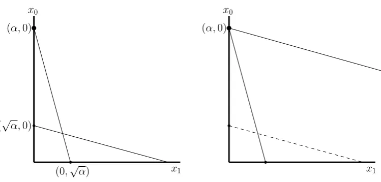
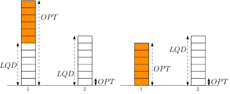
Figure 2.1: In the above example for linear programs with two variables, we assume that the objective function isx0+x1. The two constraints initially presented to the online algorithm arex0+√αx1≤αand √αx0+x1≤α(on the left). However the actual constraints of the linear program arex0+√αx1≤αand √αx0+x1 ≤α√α (on the right). The optimal point (α,0) is on the x0 axis, hence an optimal offline algorithm will only increase the value of variablex0 and leave the value ofx1 equal to 0.
network is defined as the time from the first broadcast performed anywhere in the
network, until the first battery becomes exhausted.
In this case and assuming that all entries of the matrixA are positive, each
component of the right-hand sides of the constraints of the linear program
corre-sponds to the lifetime of one battery powering a network sensor. We assume that
we are aware of the lower bounds of the remaining battery lifetimes, but the actual
remaining battery lifetimes are supposed to be within a fixed factor α > 1 of the
revealed battery lifetime values. Given this information, our objective is to choose
amongst a set of broadcasting scenarios so that the number of performed network
broadcasts is maximized, before a battery becomes exhausted.
Ochel at al. provide a Θ(lnα
α )-competitive deterministic online algorithm
for this problem and prove that any online algorithm, whether deterministic or
randomized, isO(√1
α)-competitive.
upper bound to O(d2α1/d
α ) for linear programs, having at least d variables. It is
important to note here that our upper bound is, also, dependent on the number of
variables of the linear program and not only on the parameterα.
Our second result (Englert et al. [2014]) is an upper bound of O(m2αα1/m)
on the competitive ratio of any randomized online algorithm against an oblivious
adversary for this problem, for linear programs that involve mdm! lnαe variables,
where there also exists a dependence between the achieved upper bound and the
number of variables of the linear program.
Both of the these upper bounds become O(ln2α/α) for a sufficiently large number of variables.
Finally, we give a simple deterministic Θ(√1
α)-competitive algorithm for
lin-ear programs that have d = 2 variables (Englert et al. [2014]). This algorithm is
optimal for the special case of linear programs involving exactly two variables since
its competitive ratio matches the upper bound ofO(√1
α) that has been established
by Ochel et al.
2.2
The upper bound for deterministic online algorithms
In the current section, we shall prove the next theorem.
Theorem 2.1. The competitive ratio of any deterministic online algorithm for the problem of packing linear programs with at leastd≥2 variables, is O(d2α1/d
α ).
Since the bound of Theorem 2.1 is minimized for a number of variables equal
tod= Θ(lnα), we have the next corollary.
Corollary 2.2. The competitive ratio of any deterministic online algorithm for the problem of packing linear programs, isO(ln2α
α ).
We proceed with the construction of the adversary to prove Theorem 2.1. As
to the online player by the adversary. Once the online player has increased a variable
so much that the revealed remaining slacks of some constraints become sufficiently
small, the adversary decides that these constraints are exactly those constraints for
which the revealed right-hand sides were already quite close to the true right-hand
sides, i.e., to the respective components of the capacity vectorc. As a consequence,
the value of this variable cannot be increased much further in the future and the
online algorithm is left, more or less, with a similarly constructed linear program,
but for the remaining variables.
Hence, the initial linear program presented to the online algorithm is the
following:
max
d−1 X
i=0
xi
∀permutationsπ :
d−1 X
i=0
αi/d·xπ(i)≤α
x0, x1, . . . , xd−1≥0
Our construction uses exactly d variables. Theorem 2.1 follows, since any
additional variables xd, xd+1, . . . can be made irrelevant by adding to the linear program constraints of the formxd+1≤0,xd+2≤0, etc.
The adversary maintains a set ofactive constraints and a set ofactive vari-ables. Initially all d! constraints and all d variables are considered to be active.
From the point in time when a constraint or a variable becomes inactive, this
con-straint or variable, respectively, will never become active until the online algorithm
terminates.
The adversary proceeds in d rounds, which are numbered downwards as
d−1, d−2, . . . ,0. The roundr ∈ {0, . . . , d−1}ends in the first point in time when
αr/d. At the end of roundreach of the next steps takes place in the following order:
• The adversary determines the index kr of the active variable which has the
maximum value among all variables that are currently active, breaking ties
arbitrarily.
• The adversary increases the right-hand side (i.e., the respective component
of `t) of all active constraints that do not correspond to permutations with
π(r) = kr, to α ·αr/d. Note that this does not violate the condition that
revealed remaining slacks always have to be an α-approximation of the true
remaining slacks, since all these constraints have a revealed remaining slack
which is at least equal toαr/d.
• The adversary removes from the set of active constraints all the constraints
that their right-hand side was increased in the previous step of the current
round.
• The adversary removes the variable with indexkr from the set of active
vari-ables and the current round completes.
Before continuing, we note that we may assume that the online algorithm
ends its computation after alldrounds are completed, i.e., when no variable is active
any more. This is because, for any online algorithm that terminates before round 0
is complete, there exists an other online algorithm that acts exactly as the former
online algorithm until the point in time that this former algorithm terminates and
which obtains at least the same online profit, since no variable value may decrease.
We start our proof with two easy observations. First of all, recall that at
roundr we increase the right-hand sides of all active constraints that do not
corre-spond to permutations for which it holds π(r) =kr and we, subsequently, remove
these constraints from the set of active constraints. Taking into consideration the
Observation 2.3. A permutation π corresponds to a constraint active in round r
if and only if it holds π(s) =ks for all s > r.
Now, letxr
i be the value of the variable xi at the end of round r, for i, r ∈
{0, . . . , d−1}. Since for non-negative numbers α0 ≥ α1 ≥ . . . and non-negative numbersbi, we have that the quantityPiαi·bπ(i)is maximized ifbπ(0)≥bπ(1) ≥. . ., we obtain the next observation.
Observation 2.4. Let r = 0, . . . , d−1 be a round. Also, let π be a permutation corresponding to a constraint active in roundr, such that it holds
xrπ(r)≥xrπ(r−1)≥. . .≥xrπ(0).
Note that such a permutation exists due to Observation 2.3. Then, the constraint corresponding toπ has the smallest revealed remaining slack among all permutations active in round r.
Now, for any round r = 0, . . . , d−1, let πr denote the permutation
corre-sponding to the constraint that causes roundrto end. According to Observation 2.4
we obtain:
xrπ
r(r)≥x
r
πr(r−1)≥. . .≥x
r
πr(0) (2.5)
and, therefore, we may assume from now, without loss of generality, that it holds
πr(r) =kr.
Lemma 2.6. For any round r < d−1 we have
xrπ
r(i)≥x
r+1
πr+1(i)
for anyi= 0, . . . , d−1.
Due to Observation 2.3, we haveπr(i) =πr+1(i) =ki for anyi > r+ 1 since
the constraints corresponding toπrandπr+1are both active in roundsd−1, . . . , r+1. Sinceπr(i) is, also, active in roundrand it holdsπr+1(r+1) =kr+1as already argued after (2.5), we haveπr(i) =πr+1(i) =kifori=r+ 1. Taking into consideration the
fact that variable values can only increase, this implies for i≥ r+ 1 that it holds
xr
πr(i)=x
r ki ≥x
r+1
ki =x
r+1
πr+1(i). This completes the proof for the case that i≥r+ 1.
Now, assume that i ≤ r. Since πr(i) = πr+1(i) = ki for i > r + 1, the
sequence πr+1(r+ 1), πr+1(r), . . . , πr+1(0) is a permutation of the sequence πr(r+
1), πr(r), . . . , πr(0). Therefore, the sets of variables {xπr+1(r+1), . . . , xπr+1(0)} and
{xπr(r+1), . . . , xπr(0)} are identical. Hence, since variable values can only increase,
the sequence
xrπr(r+1)≥xrπr(r)≥. . .≥xrπr(0)
is obtained from the sequence
xrπ+1
r+1(r+1)≥x
r+1
πr+1(r)≥. . .≥x
r+1
πr+1(0)
by increasing the values of one or more variables and rearranging the sequence so
that it becomes sorted. Hence, the claim follows for the case thati≤r, completing
the proof.
We can now show the next key lemma.
Lemma 2.7. For any round r∈ {0, . . . , d−1}andi≤r, it isxr
πr(i)≤(d−r)·α
1/d.
Proof. We shall use downward induction onr. The claim is clear forr=d−1, since during roundd−1 all constraints still have right-hand sides equal toα and for any
variablexi there is a constraint that contains this variable with a coefficient equal
toα1−1/d.
Consider, now, any round r < d−1. We can, easily, obtain the following
d−1 X
i=0
αi/d·xrπr(i) =
d−1 X
i=0
αi/d·xrπ+1
r+1(i)+
d−1 X
i=0
αi/d·xrπr(i)−xrπ+1
r+1(i)
(2.8)
The first sum of the right-hand side of (2.8) is lower-bounded byα−α(r+1)/d
by the definition of permutation πr+1. Moreover, by Lemma 2.6 we have xrπr(i) ≥
xrπ+1
r+1(i) for any i= 0, . . . , d−1. Therefore we have the next inequality:
d−1 X
i=0
αi/d·xrπr(i)≥α−α(r+1)/d+
d−1 X
i=0
αi/d·xrπr(i)−xrπ+1
r+1(i)
with all the terms in the sum of its right-hand side, being non-negative. Since the
constraint corresponding toπr is active and feasible in round r, the left-hand side
of the last inequality is upper-bounded by α. By ignoring all terms except the one
corresponding toi=r in the sum of its right-hand side we obtain:
xrπr(r) ≤xrπ+1
r+1(r)+
α(r+1)/d αr/d =x
r+1
πr+1(r)+α
1/d
≤(d−r)α1/d (2.9) where the last inequality of (2.9) follows from induction.
Overall, we havexr
πr(r)≤(d−r)α
1/d. By this and (2.5), we obtain the lemma
forxr
πr(i) when i < r.
Now, let us denote asx0i (where i= 0, . . . , d−1) the final value of variable
xi, that is the value of xi when the online algorithm terminates. Due to the next
lemma, we can upper-bound the online profit which equalskx0k
1, wherek.k1 denotes theL1-norm andx0 denotes the vector (x00, ..., x0d−1).
Lemma 2.10. It holds x0i =O(dα1/d) for any i= 0, . . . , d−1.
Proof. The last round performed is round r = 0, which means that there exists a constraint for which the right-hand side is set equal toα·α0/d=αat the end of this
to this constraint.
Note that no variable is active at the end of round 0 and each variable has
an indexkj =πj(j) =π(j) for some j≥0. We have:
d−1 X
i=0
αi/d·x0π(i) =
d−1 X
i=0
αi/d·xjπ
j(i)+
d−1 X
i=0
αi/d·x0π(i)−xjπ
j(i)
(2.11)
According to the definition ofπ, we obtain the next inequality as in the proof
of Lemma 2.7:
d−1 X
i=0
αi/d·xjπ
j(i)≥α−α
j/d (2.12)
Taking into consideration the fact that the sum in the left-hand side of (2.11)
is at most α, since the right-hand side of this constraint is not altered and stays
equal to α, we have from (2.11) and (2.12), similarly to the reasoning in the proof
of Lemma 2.7:
x0kj ≤xjk
j+
αj/d
αj/d ≤(d−j)α
1/d+ 1.
where we used Lemma 2.7 in order to upper-bound xjk
j in the last inequality. This
completes the proof.
In the next lemma, we bound the profit that an optimal offline algorithm
can achieve.
Lemma 2.13. An optimal offline algorithm can obtain a profit of α.
Proof. An offline algorithm can set the value of the variablexk0 equal toαand each
of the other variable values equal to 0. We shall now show that this is a feasible
solution.
For any i ≥ 1, consider any of the (d−1)! constraints in which xk0 has a
coefficient equal toαi/d. In other words, a constraint corresponding to a permutation
sinceπ(i) =k0 6=ki. Due to the strategy of the adversary, this means that, once the
constraint becomes inactive, the right-hand side increases to α·αi/d and therefore
the constraint is satisfied.
The constraints in which the coefficient of xk0 is 1 are clearly satisfied as
well, since the right-hand side of all constraints is at leastα.
By combining Lemmas 2.10 and 2.13 we obtain Theorem 2.1. This completes
the analysis for the competitive ratio upper bound for the case of deterministic online
algorithms.
2.3
The upper bound for randomized online algorithms
The upper bound on the competitive ratio of randomized online algorithms against
oblivious adversaries is based on the construction from Section 2.2. Recall that,
according to the adversary construction from this section, each round ends when
the revealed remaining slack of at least one active constraint drops below a certain
threshold value. Then, the adversary identifies the active variable having the
great-est value and increases appropriately the right-hand sides of specific constraints.
The identified variable becomes inactive from this point and on and, hence, its
value cannot be further increased much, until the online algorithm completes its
computation.
To obtain our upper bound on randomized algorithms, we shall use Yao’s
principle, which is an elegant and very useful tool in obtaining bounds for the
competitive ratio of any randomized online algorithm against oblivious adversaries.
Since an oblivious adversary is weaker than any adaptive adversary, as already
mentioned in Chapter 1, these bounds hold for randomized online algorithms against
any type of adversary.
The first application of Yao’s principle, related to theoretical computer
is, in fact, much older and can be traced back to the Minimax Theorem of von
Neumann [1928].
Assuming that P is a cost minimization online problem, letting {ALGn}
denote the set of deterministic online algorithms forP (wheren∈N) and assuming
that OPT is an optimal offline algorithm for P, then Yao’s principle states the
following:
Theorem 2.14. If Z is a probability distribution over a set of input instancesσx to
P and there exists ac≥1such that it holdsinfn∈NEZ[ALGn(σx)]≥c·EZ[OPT(σx)],
thenclower-bounds the competitive ratio of any randomized online algorithm against an oblivious adversary, for P.
For the case of a profit maximization online problemP0 and assuming that
{ALGl} (where l ∈ L) denotes the set of deterministic online algorithms for this
problem whilstOPTdenotes an optimal offline algorithm for it, Yao’s principle can
be stated as in the following:
Theorem 2.15. If Z is a probability distribution over a set of input instances σx
to P0 and there exists a positive p ≤ 1 such that it holds supl∈LEZ[ALGl(σx)] ≤ p·EZ[OPT(σx)], thenp upper-bounds the competitive ratio of any randomized online
algorithm against an oblivious adversary, for P0.
In simple words, Yao’s principle enables us instead of proving bounds for
randomized online algorithms, to construct an input distribution which, in
expec-tation, foils any deterministic online algorithm for the same online problem. Since
for the case of randomized algorithms, it is usually more difficult to bound the
ex-pected cost (or, respectively, profit) compared to the case of deterministic online
algorithms, Yao’s principle simplifies analyses substantially.
Now, let us turn to our problem of packing linear programs. The analysis of
the previous section involves a constant interaction between the online player and
by an update of the right-hand sides of specific constraints of the linear program,
by the adversary.
Recall from the introductory Chapter 1 that in order to define oblivious
adversaries, we need to allow the adversary to fix his complete behavior in advance;
it follows that we have to remove this interaction between the adversary and the
online player.
For this, the input will consist, as before, of a packing linear program, whose
constraints are given byAx≤c. Additionally, for each constrainti∈ {0, . . . , m−1},
the adversary specifies a monotonically increasing function `i(λi) of the left-hand
side of the constraint λi := (Ax)i. This function models the right-hand side of the
constraint in dependence of the current value of the left-hand side. This function
has to satisfy equality`i(λi) =ci forλi ≥ci and inequalityci−λi ≤α·(`i(λi)−λi)
forλi < ci.
Ifλi is the current value of the left-hand side of thei-th constraint, then the
online player is aware of all values of`i(z) for z≤λi but is not aware of any values
forz > λi.
Note that we only need basic threshold functions to construct the
determin-istic upper bound from the previous section. For this, we define functionsfj(λ), for
j∈ {0,1, . . . , d−1}, as
fj(λ) :=
α , λ < α−αj/d
α1+j/d , λ≥α−αj/d
The linear program is the same as the one in the previous section. The
monotonically increasing function assigned to a constraint that corresponds to
per-mutationπ, isfrifris the largest integer such thatπ(r)6=kr, wherekris the index
of the largest active variable at the end of roundr.
in order to apply Yao’s principle.
Now, in the construction of the adversary of the previous section, the order in
which the variables become inactive defines a permutationπoof the set{0, . . . , d−1}.
In other words, if the variable with index kr becomes inactive in round r we have
πo(r) = kr. Consider an adversary that acts in exactly the same way as before,
but he guesses the permutation πo and proceeds as if the variables would actually
become inactive in this order.
If the adversary guesses correctly, the construction works as intended and
the algorithm can only obtain a value of O(d2α1/d), while the optimal value is α.
If, however, the adversary chooses the permutation uniformly at random, then the
success probability is 1/(d!), that is with this probability, the same upper bound as
in the previous section is achieved. However, if the adversary guesses incorrectly the
algorithm can perform better than O(d2α1/d) and even obtain a value of α, while
the optimal value remainsα.
We are not going to analyze the average performance of an algorithm in the
setting described in the previous paragraph. Instead, we will increase the success
probability for the adversary from 1/(d!) to almost 1−1/α. This is done in a
similar way to the one that Ochel et al. provide their upper bound for randomized
online algorithms against oblivious adversaries. More specifically, we work as in the
following.
We assume that we have K adversaries with random πo sequences working
in parallel and require the online algorithm to beat all of them, for some sufficiently
largeK. Hence, suppose we want to haveK d-dimensional adversaries. We construct
a packing linear program with dK variables {x
i1,...,iK|0≤i1, . . . , iK ≤d−1}. The
objective function is the sum of all variables.
For the k-th adversary, we add d! constraints to the linear program. The
constraints have the same form as the ones in the previous section but instead of
xkj := X (i1,...,iK):ik=j
xi1,...,iK (2.16)
For each adversaryk∈ {1, . . . , K}, a permutationπkof the set{0, . . . , d−1}
is chosen independently and uniformly at random and the functionsfr are randomly
assigned to constraints based on this permutation, as described earlier.
For any adversaryk, the objective function is:
X
0≤i1,...,iK≤d−1
xi1,...,iK =
d−1 X
j=0
xkj (2.17)
Therefore, the objective function is also equal to minkPdj=0−1xkj.
We allow the online player to increase the value of xk
j directly instead of
increasing the values of the underlying xi1,...,iK variables. Note that, in reality, an
algorithm cannot increase thexk
j variables completely independently of each other,
since increasing one of the underlying xi1,...,iK variables always affects multiple x
k j
variables. However, allowing the online player to directly and individually increase
xk
j variables can only provide him with more power.
This completes the construction of an input that combines K adversaries
from the previous section, each of them independently guessing a random order in
which variables become inactive. The profit of the online algorithm against one of
the adversaries is bounded byO(d2α1/d) with probability 1
d! (that is, if the adversary guessed the correct permutation) and byα with probability (1− 1
d!).
The total profit of the online algorithm is bounded by the minimum profit
the algorithm achieves against any of theKadversaries, since the objective function
equals minkPdj=0−1xjk. Hence, by choosing K =dd! lnαe we get that the expected
overall profit of the online algorithm is bounded by:
1− 1
d! K
α+1−1− 1
d! K