University of Warwick institutional repository:
http://go.warwick.ac.uk/wrap
A Thesis Submitted for the Degree of PhD at the University of Warwick
http://go.warwick.ac.uk/wrap/60463
This thesis is made available online and is protected by original copyright.
Please scroll down to view the document itself.
T H E U N I V E R S I T Y O F
WARWICK
Library Declaration and Deposit Agreement
1. STUDENT DETAILS
Please complete the following:
2. THESIS DEPOSIT
2.1 I understand that under my registration at the University, I am required to deposit my thesis with the University in BOTH hard copy and in digital format. The digital version should normally be saved as a single pdf file.
2.2 The hard copy will be housed in the University Library. The digital version will be deposited in the University's Institutional Repository (WRAP). Unless otherwise indicated (see 2.3 below) this will be made openly accessible on the Internet and will be supplied to the British Library to be made available online via its Electronic Theses Online Service (EThOS) service.
[At present, theses submitted for a Master's degree by Research (MA, MSc, LLM, MS or MMedSci) are not being deposited in WRAP and not being made available via EthOS. This may change in future.]
2.3 In exceptional circumstances, the Chair of the Board of Graduate Studies may grant permission for an embargo to be placed on public access to the hard copy thesis for a limited period. It is also possible to apply separately for an embargo on the digital version. (Further information is available in the Guide to
Examinations for Higher Degrees by Research.)
2.4 If you are depositing a thesis for a Master's degree by Research, please complete section (a) below.
For all other research degrees, please complete both sections (a) and (b) below:
(a) Hard Copy
I hereby deposit a hard copy of my thesis in the University Library to be made publicly available to readers (please delete as appropriate) EITHER immediately OR after on embargo period of
• months/yeare as agreed by tho Chair of tho Board of Graduate Studies.
I agree that my thesis may be photocopied. YES /•WQ'(Please delete as appropriate)
(b) Digital Copy
I hereby deposit a digital copy of my thesis to be held in WRAP and made available via EThOS.
Please choose one of the following options:
EITHER My thesis can be made publicly available online. YES /( P l e a s e delete as appropriate) OR My thesis can be made publicly available only after [date] (Please give date)
OR My full thesis cannot be made publicly available online but I am submitting a separately identified additional, abridged version that can be made available online.
YES / NO (Please delete as appropriate)
YES-/ NO (Please delete as appropriate)
3. GRANTING OF NON-EXCLUSIVE RIGHTS
Whether I deposit my Work personally or through an assistant or other agent, I agree to the following:
Rights granted to the University of Warwick and the British Library and the user of the thesis through this
agreement are non-exclusive. I retain all rights in the thesis in its present version or future versions. I
agree that the institutional repository administrators and the British Library or their agents may, without
changing content, digitise and migrate the thesis to any medium or format for the purpose of future
preservation and accessibility.
4. DECLARATIONS
(a) I DECLARE THAT:
• I am the author and owner of the copyright in the thesis and/or I have the authority of the
authors and owners of the copyright in the thesis to make this agreement. Reproduction
of any part of this thesis for teaching or in academic or other forms of publication is
subject to the normal limitations on the use of copyrighted materials and to the proper and full acknowledgement of its source.
• The digital version of the thesis I am supplying is the same version as the final,
hard-bound copy submitted in completion of my degree, once any minor corrections have been
completed.
• I have exercised reasonable care to ensure that the thesis is original, and does not to the
best of my knowledge break any UK law or other Intellectual Property Right, or contain
any confidential material.
• I understand that, through the medium of the Internet, files will be available to automated
agents, and may be searched and copied by, for example, text mining and plagiarism
detection software.
(b) IF I HAVE AGREED (in Section 2 above) TO MAKE MY THESIS PUBLICLY AVAILABLE
DIGITALLY, I ALSO DECLARE THAT:
• I grant the University of Warwick and the British Library a licence to make available on the
Internet the thesis in digitised format through the Institutional Repository and through the
British Library via the EThOS service.
• If my thesis does include any substantial subsidiary material owned by third-party
copyright holders, I have sought and obtained permission to include it in any version of
my thesis available in digital format and that this permission encompasses the rights that I
have granted to the University of Warwick and to the British Library.
LEGAL INFRINGEMENTS
I understand that neither the University of Warwick nor the British Library have any obligation to take legal
action on behalf of myself, or other rights holders, in the event of infringement of intellectual property
rights, breach of contract or of any other right, in the thesis.
Please sign this agreement and return it to the Graduate School Office when you submit your thesis.
Analysis and optimisation of ground based
transiting exoplanet surveys
by
Simon Robert Walker
Thesis
Submitted to the University of Warwick
for the degree of
Doctor of Philosophy
Astronomy and Astrophysics
Contents
List of Tables v
List of Figures vi
Acknowledgments x
Declarations xi
Abstract xii
Abbreviations xiii
Chapter 1 Introduction 1
1.1 Extrasolar planets . . . 1
1.2 Detection . . . 2
1.2.1 Radial velocity . . . 3
1.2.2 Transits . . . 6
1.2.3 Microlensing . . . 9
1.2.4 Direct imaging . . . 11
1.2.5 Pulse timing . . . 13
1.2.6 Astrometry . . . 14
1.3 Planet characterisation . . . 14
1.4 Projects . . . 18
1.4.1 WASP . . . 18
1.4.2 Kepler . . . 21
1.4.3 HARPS . . . 24
1.5 Planetary formation . . . 25
1.5.1 Core accretion . . . 25
1.5.2 Gravitational collapse . . . 27
1.6.1 Disc migration . . . 28
1.6.2 Dynamical scattering . . . 31
1.7 Competing theories . . . 32
1.8 Overall properties of exoplanet populations . . . 34
1.9 Selection biases . . . 37
1.10 Instrument technology . . . 37
1.10.1 Charge Coupled Devices . . . 37
1.10.2 Calibration procedure . . . 38
1.10.3 Estimating the brightness of an object . . . 39
1.10.4 Sources of uncertainty . . . 40
1.11 Thesis structure . . . 42
Chapter 2 Quantifying the WASP selection effects 43 2.1 Motivation . . . 43
2.2 WASP project description . . . 47
2.2.1 Hardware . . . 47
2.2.2 Data reduction pipeline . . . 48
2.3 Calculating the selection effects . . . 51
2.3.1 Overview . . . 51
2.3.2 Simulation parameters . . . 52
2.3.3 Other parameters . . . 53
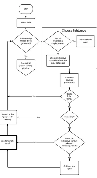
2.3.4 Lightcurve synthesis . . . 54
2.3.5 Testing the transit synthesis method . . . 57
2.3.6 Model rejection . . . 59
2.3.7 Implementation of the data modification process . . . 60
2.3.8 Testing and verification . . . 62
2.4 Computing the sensitivity map . . . 64
2.4.1 Acceptance . . . 66
2.4.2 Selection cuts . . . 67
2.4.3 Period matching . . . 70
2.5 Sensitivity maps . . . 71
2.5.1 Planet trends . . . 71
2.5.2 Shaping the sensitivity map . . . 73
2.5.3 Combining individual sensitivity measurements . . . 76
Chapter 3 Determining the underlying population of hot Jupiters
using the WASP survey 81
3.1 Modifications for analysing the full WASP stellar sample . . . 82
3.1.1 Composing a sample of stars . . . 82
3.1.2 Calculating unknown stellar parameters . . . 84
3.1.3 Analysis pipeline modifications . . . 86
3.2 Shaping the sensitivity map . . . 87
3.3 Sensitivity maps . . . 89
3.3.1 Incorporating probability of transit . . . 95
3.4 Comparing input systems to detections . . . 95
3.5 Constraining the underlying hot Jupiter population . . . 97
3.5.1 Joint constraint with Kepler . . . 99
3.5.2 A new model for the underlying period distribution . . . 105
3.5.3 Investigating the radius distribution . . . 110
3.6 Discussion . . . 112
Chapter 4 NGTS: Design and prototype 117 4.1 Introduction . . . 117
4.2 Achieving the targets . . . 120
4.2.1 Design . . . 120
4.2.2 Prototype testing . . . 123
4.3 La Palma prototype . . . 123
4.3.1 Aperture photometry implementation . . . 126
4.3.2 Removing trends . . . 133
4.3.3 Limitations . . . 134
4.4 Noise model . . . 135
4.5 Prototype results . . . 138
4.5.1 Precision . . . 138
4.5.2 Noise colour . . . 142
4.5.3 PSF sensitivity . . . 144
4.5.4 Blending . . . 147
4.6 Summary . . . 151
Chapter 5 NGTS final instrument and planet catch simulations 154 5.1 The NGTS project . . . 154
5.2 Reapplication of the noise analysis . . . 155
5.2.1 Updated noise model . . . 156
5.3 Camera testing . . . 162
5.3.1 Streak characterisation . . . 163
5.3.2 Dark current measurement . . . 165
5.4 Optimising the observing strategy . . . 167
5.4.1 Saturation levels . . . 168
5.4.2 Exposure time optimisation . . . 171
5.5 Planet catch . . . 173
5.6 Summary . . . 180
Chapter 6 Conclusions and future work 183 6.1 Determining the underlying population of hot Jupiters with the WASP project . . . 183
6.2 The Next Generation Transit Survey . . . 184
6.3 Future work . . . 185
List of Tables
2.1 Literature hot Jupiter occurrence rates. . . 46
2.2 Limb darkening coefficients for three example temperatures . . . 56
3.1 Parameter cuts used to restrict the WASP stellar sample. . . 84
3.2 Properties of the Kepler stellar and planetary sample. . . 100
3.3 Best fit parameters of the period model. Taken from Howard et al. [2012]. . . 101
3.4 Best fit parameters for the power law model with Gaussian excess calculated from minimising the least squares. . . 107
3.5 Best fit parameters for the model (Eq. 3.8). The previous values from Table 3.4 have been repeated for comparison. . . 109
3.6 Cash best fit radius parameters . . . 110
4.1 Comparison of detector features . . . 125
4.2 Sky background values for days since New Moon, for La Palma . . . 137
4.3 Coordinates of the fields used for the crowding analysis . . . 150
5.1 Comparison of NGTS detector features . . . 155
5.2 Saturation coefficients for a given exposure time . . . 170
5.3 Coordinates used for the NGTS planet catch simulations . . . 175
5.4 Coefficients used for the Kepler occurrence rate . . . 175
List of Figures
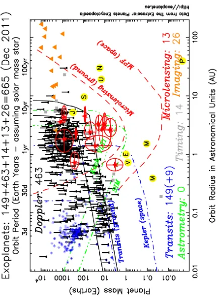
1.1 Orbital separation and planetary mass for the known exoplanets as
of December 2011. . . 4
1.2 Radial velocity examples . . . 5
1.3 Discovery transit data for HD 209458 b . . . 6
1.4 Transit geometry schematic . . . 8
1.5 Microlensing examples . . . 10
1.6 Image of Fomalhaut . . . 13
1.7 Rossiter-McLaughlin example . . . 16
1.8 Distribution of spin orbit alignments . . . 16
1.9 Examples of atmospheric characterisation . . . 17
1.10 The WASP-South instrument . . . 19
1.11 Transit of HD 209458 b from the WASP0 prototype . . . 20
1.12 Transit of WASP-1 b taken with the WASP instrument . . . 21
1.13 Examples of Kepler transits . . . 23
1.14 Simulations of a protoplanetary disk showing gravitational instability 28 1.15 Simulation of Type II migration . . . 30
1.16 Distribution of known planetary orbital periods . . . 34
1.17 Orbital eccentricity and metallicity measurements for known exoplanets 35 1.18 Mass-radius relations . . . 36
1.19 Analogy of a CCD . . . 38
1.20 Geometry of a photometric aperture with its annulus. . . 40
2.1 Hot Jupiter distributions . . . 45
2.2 Geometry of limb darkening . . . 55
2.3 Synthetic stellar profiles . . . 56
2.4 Demonstration of the transit removal and synthesis process . . . 58
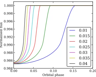
2.7 Examples of transit shapes . . . 64
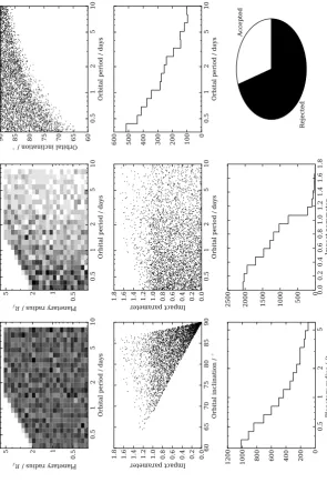
2.8 Statistics of the proposed synthetic systems . . . 65 2.9 ∆χ2 periodogram for planet WASP-12 b . . . . 67
2.10 Input period against recovered period for every accepted synthetic
object . . . 70 2.11 Sensitivity maps for WASP-12 b and WASP-7 b . . . 72
2.12 Sensitivity maps generated for the WASP stars ordered by V magnitude 74
2.13 Orion detection map . . . 75 2.14 Maps made from individual selection cuts . . . 77
2.15 Combined sensitivity map for the planet hosting stars . . . 78
2.16 One dimensional sensitivity profiles marginalised over the second axis 79
3.1 Dwarf probability used in the classification of stars for the WASP
reduced stellar input catalogue. . . 83
3.2 Distributions of the stellar parameters used to reduce the input sample 85 3.3 Distribution of the number of synthetic transiting systems inserted
per lightcurve. . . 88 3.4 oriondetection map . . . 89
3.5 Sensitivity maps made from each selection cut . . . 90
3.6 Sensitivity maps created from the two different WASP stellar samples 91 3.7 Ratio of the sensitivity maps made from the two stellar samples . . . 92
3.8 Histogram of values in the map ratio >0 . . . 92
3.9 Flattened sensitivity profile. . . 93 3.10 Sensitivity maps built up by splitting the magnitude range of study
into three . . . 94
3.11 Sensitivity map including the probability of transit . . . 96 3.12 Comparison of the proposed and best fit planetary radius . . . 97
3.13 Comparison of the input and detected impact parameters from the
analysis . . . 98 3.14 Correction factors calculated by inverting the WASP planets through
the sensitivity map. . . 99
3.15 Observed and underlying hot Jupiter distributions . . . 100 3.16 Confirmed WASP planet, and Howard et al. [2012] Kepler candidate
distributions . . . 102
3.18 Occurrence rate in planets per star showing the Kepler and WASP
results . . . 104
3.19 The occurrence rate in planets per star after increasing the bin reso-lution . . . 105
3.20 Howard et al. [2012] occurrence rate models for orbital period . . . . 106
3.21 Modelling the occurrence rate using the Howard et al. [2012] model . 107 3.22 Results for the new occurrence rate model for giant planets . . . 108
3.23 Fits to the occurrence rate of giant planets considering Poisson statistics109 3.24 Result of characterising the radius distribution . . . 111
3.25 Rotation rates for T Tauri stars in the Orion Nebula Cluster . . . . 113
3.26 Planetary mass against orbital period for planets Rp ≥8 R⊕. . . 113
3.27 Corrected Roche limit ratio distribution . . . 114
3.28 Radius for hot Jupiter planets withRp≥8R⊕. . . 115
4.1 Planet radius histogram for the known exoplanets . . . 118
4.2 Planet radii and host star radii for planets detected from the ground 119 4.3 Throughput of the NGTS instrument . . . 121
4.4 A complete NGTS unit, assembled at the Geneva Observatory. . . . 122
4.5 Weather quality for Paranal . . . 123
4.6 Computer generated renders of the NGTS facility . . . 124
4.7 Images of the NGTS prototype installed in La Palma . . . 125
4.8 Graphic representing the nights for which NGTS prototype data exists126 4.9 An example NGTS prototype image, taken on 2009-10-07 . . . 128
4.10 Example aperture used by the photometry pipeline . . . 128
4.11 QE quoted from the Andor brochure . . . 129
4.12 Histogram of the estimated zero points for the field of the night of 2009-10-07 . . . 130
4.13 Geometry of the light path length through the atmosphere, from Bir-ney et al. [2006]. . . 131
4.14 Extinction behaviour for a group of stars . . . 132
4.15 Extinction measurements from the Carlsberg Meridian Telescope . . 133
4.16 sysremcoefficients for 2009-11-19 . . . 134
4.17 Example lightcurve from 20010-02-04 . . . 136
4.18 Sky background measurement from the NGTS prototype . . . 137
4.19 Noise model for the NGTS prototype . . . 139
4.20 Properties of the NGTS prototype dataset . . . 140
4.22 Measured fractional noise values for the night of 2009-11-19 . . . 143
4.23 Binned median precision of bright stars . . . 144
4.24 Example data from a single lightcurve collected during 2009-10-07. . 145
4.25 Examples of the focus levels shown in Fig. 4.20 . . . 146
4.26 PRF responses . . . 148
4.27 NGTS yearly coverage . . . 149
4.28 Histogram of the fraction of objects which are un-blended . . . 150
4.29 Transits observed by the NGTS prototype . . . 152
5.1 Comparison of noise models for the prototype and Geneva instruments157 5.2 Binned noise models for NGTS for a range of stellar magnitudes . . 159
5.3 Binned noise models for NGTS for a range of exposure times . . . . 160
5.4 Fractional rms for the data collected at Geneva on 2012-08-17 . . . . 161
5.5 Binned fractional rms of stars with magnitudes 11≤I ≤8 . . . 162
5.6 Example streaks from on-sky data . . . 163
5.7 Example of the two sided CCD sensitivity . . . 165
5.8 Streak examples . . . 166
5.9 Illuminated region of the CCD tested at Leicester . . . 166
5.10 Median dark current values at different temperatures . . . 168
5.11 Schematic of a Gaussian centred at (0.3, 0.3), and a FWHM of 1.5 pixels . . . 169
5.12 Distribution of pixel flux fractions from a Monte Carlo simulation . . 170
5.13 Saturation behaviour with exposure time . . . 171
5.14 The calculated high precision region . . . 172
5.15 Analysis of optimising the exposure time . . . 174
5.16 Assumed period window function for the NGTS project. . . 176
5.17 Planet catch simulations in units of velocity semi major amplitude . 179 5.18 Planet catch simulation results in units of planet radius . . . 180
A.1 Sensitivity maps in order of Tef f. . . 188
A.2 Sensitivity maps in order of Metalicity. . . 189
A.3 Sensitivity maps in order of R?. . . 190
Acknowledgments
I’d like to thank my supervisor Dr. Peter Wheatley, without whom this thesis
definitely would not be possible. His support and assistance during the course of my
PhD were invaluable. Thanks to everyone in the Astronomy and Astrophysics group
at Warwick, who have provided a constant stream of support and entertainment.
I want to thank both the WASP and NGTS consortiums for making this work
possible, especially the members who I have worked directly with: Dr. Richard
West and Prof. Don Pollacco.
I’d like to thank my parents for both supporting me during both the happy
and stressful times, and for being wonderful. I would not be where I am today
without them. Without good office mates, a person may go slightly insane.
Alter-nativelywith good office mates a person may go slightly insane. Whichever is more
appropriate I’ve had fantastic office mates, and special thanks goes to Jon, Lieke,
Tom and Jo˜ao. In particular, without Jo˜ao I could not have achieved quite so much,
and would not have discovered some fantastic music. I’d like to thank my friends
and fellow year-mates Rachel, Matt, Steve and Pete for countless hours of laughter.
And finally I’d like to thank my girlfriend Zoe who has been wonderful, managed
Declarations
I declare that the work presented in this thesis is my own except where stated
oth-erwise, and was carried out entirely at the University of Warwick, during the period
October 2009 to May 2013, under the supervision of Dr. Peter Wheatley. Work
in Chapters 4 and 5 were carried out as a member of the NGTS consortium. The
research reported here has not been submitted, either wholly or in part, in this or
any other academic institution for admission to a higher degree.
Contributions based on this thesis are:
• National Astronomy Meeting, Manchester, UK, March 2012, Poster presenta-tion: Selection effects of the SuperWASP project.
• International Astronomical Union Symposium 299, Victoria, Canada, June 2013, Poster presentation: Determining the population and evolution of hot
Abstract
One of the most surprising aspects of the exoplanet population is the exis-tence of Jupiter sized planets orbiting close to their parent stars. It is currently uncertain how these planets reached such small separations, and they are thought to be markers for the dominant migration mechanism. The Wide Angle Search for Planets (WASP) project is ideally suited for studying these planets, as it has de-tected the largest number of hot Jupiters to date. I have inverted the observed sam-ple of WASP planets to calculate the underlying population of hot Jupiters through a quantitative study of the selection biases in the WASP project. To achieve this, I synthesised transiting systems and inserted them into WASP data to calculate the probability of detection. The observed population of WASP planets is then corrected through application of this probability to determine the underlying population. I find a clear pile up in the underlying population at orbital periods between 3 to 5 days, and apply a joint constraint with the underlying population measurement from the Kepler project to propose a new model for the underlying population of giant planets. I propose a model consisting of a rising power law win period with index 1.0±0.3, with a Gaussian excess at 3.7±0.1 days to model the period pile up. The observed period pile up places crucial constraints on models of hot Jupiter migration.
Abbreviations
WASP Wide Angle Search for Planets
NGTS Next Generation Transit Search
PSF Point Spread Function
PRF Pixel Response Function
CCD Charge Coupled Device
FWHM Full Width Half Maximum
ESO European Southern Observatory
RMS Root Mean Squared
ADU Analogue-to-Digital Unit
FOV Field Of View
RV Radial Velocity
KIC Kepler Input Catalogue
CTE Charge Transfer Efficiency
R Solar radius, 7.955×10⁵km
RJ Jupiter radius, 71 492 km
M Solar mass, 1.989×1030kg
MJ Jupiter mass, 1.898×1027kg
M⊕ Earth mass, 5.972×1024kg
Chapter 1
Introduction
1.1
Extrasolar planets
Planets that exist outside our Solar System and therefore do not orbit the Sun are classed as extra-solar planets, or exoplanets. Exoplanets had been predicted [e.g.
Newton, 1726, and before], but the first discovery of an exoplanet was in 1992 by Alex
Wolszczan and Dale Frail around the millisecond pulsar PSR1257+12 [Wolszczan & Frail, 1992]. Since then 986 exoplanets have been confirmed as of 2013/9/301.
With increasing numbers of exoplanets and exoplanetary systems comes a
greater understanding of their population and formation, but they are full of sur-prises. The first exoplanet detected around a Sun-like star 51 Peg, by Mayor &
Queloz [1995] was found to be a half Jupiter mass planet orbiting at a distance
seven times closer than Mercury to the Sun. This class of planet has no analogue in the Solar System and was a curious case.
The hot Jupiter class of planet that includes this example is loosely defined as planets with similar mass to Jupiter, orbiting their parent star in less than 10
days. These planets were first to be discovered due to their large radial velocity
signal and then large transit signature (see Section 1.2), and are strongly selected for in radial velocity and especially transit surveys.
The exoplanet sample now includes similar systems to 51 Peg b, but also
systems similar to the Solar System with multiple planets of different sizes, some orbiting in resonance with each other. Improved instrumentation has enabled the
detection of near-Earth sized planets (e.g. CoRoT-7 b, [Queloz et al., 2009]) at
increasing orbital periods. The huge diversity of the exoplanet population and in some cases the lack of similarity with the Solar System is extremely interesting, and
1
requires development of theories of planetary system formation to encompass both
singular hot Jupiter systems and multi-planet systems observed.
As well as studying the population, individual systems are analysed to
ascer-tain properties of the planet and its composition. With high-precision space
tele-scopes the planetary atmospheres are probed, determining the atmospheric chem-ical composition, enabling the search for dis-equilibrium chemistry and potential
biomarkers. Combining detection techniques allows for planetary density
measure-ments to be made, resulting in some planets which are more dense, and some planets that are less dense thana priori assumptions suggest.
In the following section the methods used to detect exoplanets are described.
The detection techniques often complement each other providing more information than each individual technique alone. These same techniques may also be used for
planet characterisation, and some uses of the detection techniques beyond inferring
the presence of the planet are described in Section 1.3. Some example projects of exoplanet surveys involved in the detection or characterisation of exoplanets are
described in Section 1.4. We use the observed population of exoplanets as evidence
of the formation and subsequent evolution of planets. The two primary theories for the formation of planets out of a disk of material orbiting a young star are given in
Section 1.5. The existence of hot Jupiters at distances much closer than is possible to form such large planets is compelling evidence that planets undergo migration form
their initial formation location to their observed positions. Possible mechanisms
for this process are described in Section 1.6, and a discussion of the corresponding evidence for possible formation and migration methods is given in Section 1.7. With
a statistical sample of exoplanets the population can be studied, where common
properties or behaviours can be determined. This is discussed in Section 1.8 with a corresponding caution about studying the observed population as biases exist. These
biases are due to the sensitivities exhibited by the various detection techniques, and
may cause incorrect conclusions to be drawn about population (Section 1.9). The process of performing astronomical observations, technologies used and uncertainties
therein are described in Section 1.10.
1.2
Detection
Multiple methods exist for detecting exoplanets. Different detection methods have
different regions of this parameter space where they are sensitive to detecting plan-ets. In this section some of the different detection techniques are described.
planet mass, and shows the detection limits for various detection methods.
1.2.1 Radial velocity
A body orbiting a star causes a reflex motion in the star around the centre of mass of the system which, depending on the masses and orientations involved, may be
detectable with a high-precision spectrograph.
Light from a moving object changes frequency due to the Doppler effect. The projection of this motion along the line of sight to the object causes blue and red
shifting of the light received. In the classical form the radial velocityvr is observed to be
vr≈
∆λ λem
c (1.1)
where ∆λ is the change in wavelength observed from rest frame observations λem,
andc is the speed of light.
This signal is detected through observing an object with a high-resolution spectrograph. Multiple spectra are taken of the star and radial velocity signals
are measured from the time-varying spectra. The presence of a massive body in the
system displaces the measured spectral lines from their rest wavelength in a periodic manner. To increase the precision of the radial velocity measurement, the spectral
lines are typically cross correlated with a template spectral line. This is possible
because each line is displaced by the same amount.
The eccentricityeand argument of periastronωare measured from the shape
of the radial velocity signal. A circular orbit causes a sinusoidal signal, whereas
elliptical orbits cause deviations from sinusoidal behaviour, and this deviation can be modelled through varying the ellipticity and argument of periastron. Another
key feature of the radial velocity signal is the semi-amplitude defining maximum radial velocity signal observed. The measured semi-amplitude of the periodic signal
K? along with the independently determined eccentricity and orbital period allow
the calculation of the mass ratio of the planetary system, with an uncertainty by an unknown factor due to the system inclination. The velocity semi-major amplitude
is given by
K? =
2πG P
1/3
mpsini (M?+mp)2/3
1
√
1−e2 (1.2)
[Cumming et al., 1999] where mp and M? are the masses of the planet and star,
measure-Figure
1.1:
Orbital
separation
and
planetary
mass
for
the
kno
wn
exoplanets
as
of
Decem
b
er
2011.
P
oin
ts
mark
the
detections
and
are
coloured
b
y
the
detection
tec
hnique
used
to
disco
v
er
them.
Li
nes
mark
the
p
re
d
icte
d
sensitivit
y
limits
for
the
detection
tec
hniques.
Image
courtesy
of
Keith
[image:21.595.78.519.120.711.2](a) (b)
Figure 1.2: Left: discovery data for 51 Peg b [Mayor & Queloz, 1995]. Right: ex-ample radial velocity measurements with best fit solution for HD 100777 b. The top panel shows the measured radial velocity profile, the bottom panel shows the residuals to the best fitting solution. Image from Naef et al. [2007].
ments alone, so planetary systems which are only detectable by the radial velocity
signal do not have a unique mass value, only the projected mass mpsini is
avail-able. Figure 1.2a shows the discovery data for 51 Peg b showing smooth sinusoidal variations characteristic of a massive planet on a circular orbit. Figure 1.2b shows
an example dataset collected by HARPS for the star HD 100777 around which a
planet with mass 1.16 times the mass of Jupiter (MJ = 1.90×1027kg) orbits on a 384-day orbit. The deviation from a sinusoidal shape implies an eccentric orbit;
from Keplerian modelling the eccentricity was measured to bee= 0.36±0.02 [Naef et al., 2007].
The velocity semi-amplitude is proportional to mp/P1/3 (from Eq. 1.2,
as-suming mp M?) so the radial velocity technique excels at finding large mass planets in short period orbits around their host stars. The technique does not re-quire a full period to be observed and so is also successful at detecting massive
planets relatively far from their host star, as shown in Fig. 1.1 by the large
popu-lation of planets with masses mp &100 M⊕ (M⊕ = 5.97×1024kg) at separations
a ∼ 1 AU (AU = 1.496×10¹¹m). Eccentricities e & 0.6 also pose difficulties for detecting radial velocity signals at shorter periods due to the sparse sampling of
Figure 1.3: Discovery transit data for HD 209458 b consisting of two epochs of observations overlaid in time since the mid-transit point [Charbonneau et al., 2000].
true planets may have been missed.
1.2.2 Transits
Light from a star is attenuated when a planet crosses its disk. This decrease in
flux may be observed and the presence of the planet inferred. Figure 1.3 shows the transit data for the first exoplanet detected using this method: HD 209458 b. The
maximum loss of light from a transit is
δtra ≈
Rp R?
2
1−Ip
I?
(1.3)
[Seager, 2011] where Rp is the planetary radius, R? is the stellar radius, Ip is the
flux emitted by the planet andI? the flux emitted by the star. Limb darking on the
star causes a non-uniformity across the stellar disk and changes the shape of the transit. As the deviation from normal stellar background is proportional to the ratio
of the object areas the transit signal is typically small, with even the largest planets
only causing a transit signal of a few percent. For example Jupiter crossing the Sun creates a transit signal ofδtra = (RJ/R)2 = 1.045% where R = 7.00×10⁵km.
Similarly when the planet passes behind the star a secondary eclipse occurs
with observable depth
δocc≈
Rp R?
2
Ip I?
The deviation from predicted secondary eclipse timing provides a tight constraint
on the eccentricity of the planetary orbit [Perryman, 2011].
Observing a transit requires a close alignment between the orbital plane of
the planetary system and the line of sight. Transits can only be detected within a
narrow region of orbital inclinationsi≥icwhere
sinic≥
(Rp+R?)
a (1.5)
[Seager, 2011]. A lightcurve of a transiting system provides information about the
objects contained. The orbital period of the system is measured from the time
between transit events, from which the orbital separationais calculated by substi-tuting Kepler’s third law [Haswell, 2010]:
a3
P2 =
G(M?+mp)
4π2 (1.6)
Generallymp M?, so given an estimate of the stellar mass M? (e.g. from stellar spectroscopy, or asteroseismology) the separation can be determined [Haswell, 2010]:
a≈ GM?
P 2π
2!1/3
(1.7)
Figure 1.4 illustrates the geometry of the transiting system, with impact
parameterbshowing that the planet is not passing across the centre of the star, but
is offset by projected distanceb in units of stellar radii. There are four observable quantities which characterise the duration and profile of the transit: the orbital
period P given by the spacing between transits, the transit depthδtra, the interval
between first and fourth contacts Ttot, and the interval between the second and third contacts Tf ull [Perryman, 2011]. These observables are used in the following
geometric equations [Seager, 2011]:
∆F =
Rp R?
2
(1.8)
b2 = (1−
√
δtra)2−(Tf ull/Ttot)2(1 +
√
δtra)2 1−(Tf ull/Ttot)2
(1.9)
R?
a =
π
2δtra1/4
q
Ttot2 −Tf ull2 P
1 +esinω
√
1−e2
, (1.10)
Figure 1.4: Illustration of a transit showing the geometry discussed in Section 1.2.2. Above is a schematic diagram of the transiting system seen as the planet crosses the disk of the star. Below is an idealised transit lightcurve across a uniform brightness stellar disk. Specific contact points are labelled. From Seager [2011].
With an independent estimate of the stellar radius (e.g. from stellar models) the
planetary radius can be directly obtained from Eq. 1.8. Recent development in
Bayesian techniques allow the direct estimation of the orbital eccentricity from the transiting lightcurve by using prior constraints on the host star density and studying
the posterior eccentricity distribution [Dawson & Johnson, 2012].
The transit detection process starts with searching the lightcurve of a star for a repeated box-like feature. Various algorithms for detecting transits exist [Enoch
et al., 2012], the box-least-squares (BLS) algorithm [Kov´acs et al., 2002] is the
most common and was developed to perform this and uses a grid search in orbital period, transit depth and epoch and compares the generated box feature with the
lightcurve to calculate goodness of fit. If a significant transit-like signal is found then
the planet is commonly confirmed with the radial velocity technique, providing both an independent confirmation of the validity of the system and with the full set of
system parameters solved, the candidate planet can be confirmed as a real planet or
false positive. Common false positives which give transit-like signals include shallow eclipsing binary stars, where a grazing transit can produce a∼1% repeated dip; an eclipsing binary nearby to the target star, which injects a transit-like signal into the lightcurve; or sunspots on the target star which also cause dips in flux though these
The significance of a transit-like signal is dominated by the noise level of the
lightcurve. Projects built to search for transiting planets are designed to produce the highest precision lightcurves possible. The probability that a planet will cross
the disk of a star along the line of sight from the observer is given as
p= R?
a (1.11)
calculated from the solid angle on the sphere swept out by the planet’s shadow [Per-ryman, 2011] and is generally very small even for hot Jupiters (e.g. a planet orbiting
at 0.1 AU around a 1R star has a transit probability of 4.7%) so transiting
exo-planet surveys typically aim to observe as many stars as possible simultaneously.
1.2.3 Microlensing
Under General Relativity the presence of mass deforms light travel paths through
spacetime. Similar to optical systems when an object passes behind a gravitational lens the received image is distorted and magnified. The gravitational lens in this
case is a massive object such as a star. The characteristic length scale for this
distortion is the Einstein radiusRE such that
RE =
2RS
DLDLS DS
1/2
(1.12)
whereRS is the Schwartzchild radius
RS = 2GML/c2 (1.13)
and the D terms the distances from the observer to the lens (DL), the observer
to the source DS and the distance from the lens to the source DLS. This radius characterises the Einstein ring around the lens star (see Fig. 1.5a for a schematic
of the geometry.) A lens star passing in front of a background star will cause
magnification and distortion of the background star, provided the projected angular separation between the two objects is small. The distortion causes a deviation in
the source image path, a secondary image of the source to appear on the opposite
side of the Einstein ring (I− in Fig. 1.5a) and for both images to appear distorted
from their original shape. Magnification occurs because the flux from each image
is the product of the (constant) source brightness, and solid angle subtended by
(a)
©2006Nature Publishing Group
limits on the frequency of Jupiter-mass planets have been placed over
an orbital range of 1–10AU, down toM%planets15–17for the most
common stars of our galaxy.
On 11 July 2005, the OGLE Early Warning System18
announced the microlensing event OGLE-2005-BLG-390 (right ascension
a¼17 h 54 min 19.2 s, declinationd¼2308220
3800
, J2000) with a relatively bright clump giant as a source star. Subsequently, PLANET, OGLE and MOA monitored it with their different telescopes. After
peaking at a maximum magnification ofAmax¼3.0 on 31 July 2005,
a short-duration deviation from a single lens light curve was detected on 9 August 2005 by PLANET. As described below, this deviation was due to a low-mass planet orbiting the lens star.
From analysis of colour-magnitude diagrams, we derive the following reddening-corrected colours and magnitudes for the
source star: (V2I)0¼0.85,I0¼14.25 and (V2K)0¼1.9. We
used the surface brightness relation20linking the emerging flux
per solid angle of a light-emitting body to its colour, calibrated by interferometric observations, to derive an angular radius of
5.25^0.73mas, which corresponds to a source radius of
9.6^1.3R((whereR(is the radius of the Sun) if the source star
is at a distance of 8.5 kpc. The source star colours indicate that it is a 5,200 K giant, which corresponds to a G4 III spectral type.
Figure 1 shows our photometric data for microlensing event OGLE-2005-BLG-390 and the best planetary binary lens model.
The best-fit model hasx2
¼562.26 for 650 data points, seven lens
parameters, and 12 flux normalization parameters, for a total of 631 degrees of freedom. Model length parameters in Table 1 are expressed
in units of the Einstein ring radiusRE(typically,2AUfor a Galactic
Bulge system), the size of the ring image that would be seen in the case of perfect lens–source alignment. In modelling the light curve,
we adopted linear limb darkening laws21withG
I¼0.538 and
GR¼0.626, appropriate for this G4 III giant source star, to describe
Figure 1|The observed light curve of the OGLE-2005-BLG-390 microlensing event and best-fit model plotted as a function of time.Error bars are 1j. The data set consists of 650 data points from PLANET Danish (ESO La Silla, red points), PLANET Perth (blue), PLANET Canopus (Hobart, cyan), RoboNet Faulkes North (Hawaii, green), OGLE (Las Campanas, black), MOA (Mt John Observatory, brown). This photometric monitoring was done in the I band (with the exception of the Faulkes R-band data and the MOA custom red passband) and real-time data reduction was performed with the different OGLE, PLANET and MOA data reduction pipelines. Danish and Perth data were finally reduced by the image subtraction technique19with the OGLE pipeline. The top left inset
shows the OGLE light curve extending over the previous 4 years, whereas the top right one shows a zoom of the planetary deviation, covering a time interval of 1.5 days. The solid curve is the best binary lens model described in the text withq¼7.6^0.7£1025, and a projected separation of
d¼1.610^0.008RE. The dashed grey curve is the best binary source
model that is rejected by the data, and the dashed orange line is the best single lens model.
Figure 2|Bayesian probability densities for the properties of the planet and its host star.a, The masses of the lens star and its planet (M*andMp
respectively),b, their distance from the observer (DL),c, the
three-dimensional separation or semi-major axisaof an assumed circular planetary orbit; andd, the orbital periodQof the planet. (Ina,Mrefrefers to
M%on the upper x axis andM(on the lower x axis.) The bold, curved line in
each panel is the cumulative distribution, with the percentiles listed on the right. The dashed vertical lines indicate the medians, and the shading indicates the central 68.3% confidence intervals, while dots and arrows on the abscissa mark the expectation value and standard deviation. All estimates follow from a bayesian analysis assuming a standard model for the disk and bulge population of the Milky Way, the stellar mass function of
ref. 23, and a gaussian prior distribution forDS¼1.05^0.25RGC(where
RGC¼7.62^0.32 kpc for the Galactic Centre distance). The medians of
these distributions yield a 5:5þ5:5
22:7M%planetary companion at a separation
of 2:6þ1:5
20:6 AUfrom a 0:22þ200::2111M(Galactic Bulge M-dwarf at a distance of
6.6^1.0 kpc from the Sun. The median planetary period is 9þ9
23years. The
logarithmic means of these probability distributions (which obey Kepler’s third law) are a separation of 2.9AU, a period of 10.4 years, and masses of 0.22M(and 5.5M%for the star and planet, respectively. In each plot, the
independent variable for the probability density is listed within square brackets. The distribution of the planet–star mass ratio was taken to be independent of the stellar mass, and a uniform prior distribution was assumed for the planet–star separation distribution.
LETTERS NATURE|Vol 439|26 January 2006
438
(b)
Figure 1.5: Left: geometry of the microlensing system, projected into the sky plane of the observer and reference frame of the lens objectL. The source objectS travels across the system along the source track causing the images I+ and I− to appear.
The images rotate whilst remaining on opposite sides ofLas marked by the diagonal dashed line. Image adapted from Paczynski [1996]. Right: microlensing lightcurve for OGLE-2005-BLG-390L b a 5.5 M⊕ planet [Beaulieu et al., 2006]. Inset: the
microlensing signal caused by the presence of the planet.
behind the lens along the observers line of sight. At this point the magnification of
the source is formally infinite but the alignment is never perfect as the two objects
are not points. The magnification can be large, the largest to date is a magnification of 3000±1100 times [Dong et al., 2006].
A third body such as a planet orbiting the central lens will distort the caustic
region to contain a region behind the planet, where the particular shape is deter-mined by the orbital separation of the lens star and its planet. As the planet orbits,
this region coincides with the background star to create divergence from smooth
magnification profile of the background star, and adds a feature to the otherwise smooth magnification event. Figure 1.5b shows the lightcurve for
OGLE-2005-BLG-390L where the inset shows the effect of the orbiting planet, a 5.5 M⊕ planet. The
overall smooth shape shown in the main figure is caused by the background star passing behind the lens, and the imperfection is caused as the position of the planet
during its orbit causes a caustic region to fall on the path of the background star
inducing extra magnification.
Microlensing events are rare, and occur only once per target star, so projects
provide a constant monitoring of the galactic bulge where the galactic stellar density
a microlensing event is detectable. Sumi et al. [2011] report the detection of 10
possible rogue planet events with 6 confirmed by the OGLE project and quote an abundance rate of these objects as 1.81.7
−0.8 planets per star.
1.2.4 Direct imaging
Repeated high angular resolution images of a star are taken. Planets in the
sys-tem may be detected, either through reflected light from the host star or directly detecting thermal emission from the planet. For reflected light of wavelengthλthe
planet/star flux ratio can be written
fp(α, λ) f?(λ)
=p(λ)
Rp a
2
g(α) (1.14)
wherep(λ) is the geometric albedo andg(α) is a phase dependant function ofα, the
angle between observer and star subtended at the planet [Perryman, 2011].
The planet can be approximated with a blackbody and so emits a thermal spectrum given by the Planck function
Bλ(T) = 2hc2
λ5
1
e
hc λkB T −1
(1.15)
whereBλ(T) is spectral radiance in units of W sr−1m−3 at wavelength λ, andh is
Planck’s constant,cis the speed of light,kB is Boltzmann’s constant,T is the tem-perature of the blackbody. The wavelength of maximum emission from a blackbody
is related to the temperature of the body by Wien’s displacement law
λmaxT = 2.897×10⁻³m K (1.16)
and is derived from Eq. 1.15. This relation shows that the peak emission of a cooler
body is at longer wavelength. The planetary effective temperature is lower than the stellar effective temperature so the flux ratio between planet and star is maximised
at longer wavelengths.
Combining the two effects increases the contrast ratio between planet and star, but this ratio is small as the star is typically many orders of magnitude brighter
than the planet even at favourable wavelengths, for example the Jupiter/Sun flux
ratio is ∼10−9. To reduce the stellar flux and increase the contrast ratio further, coronograph masks are employed to block the light from the central star. A physical
mask is inserted into the optical path which minimises the stellar flux, and
central mask.
Planets can only be detected through direct imaging at large separations as the glare from the star masks the flux from the planet. Atmospheric refraction and
seeing limit the minimum separation a planet is detectable. To reduce the extent
of the stellar glare a high angular resolution is required, making the planet visible. Adaptive optics, or taking observations from space e.g. the Hubble Space Telescope
(HST) are used for direct imaging observations to minimise or negate the effects of
the atmospheric refraction and seeing. The wavefront from a bright reference star or synthetic laser guide star is sampled at timescales on the order 1 ms, and correction
actuators apply the inverse wavefront to a deformable mirror in the camera system.
By correcting for atmospheric turbulence the angular resolution can be increased to the diffraction limit of the telescope. The angular resolution is approximated by
R≈1.22λ
D (1.17)
whereDis the diameter of the telescope aperture. By using large aperture telescopes
the angular resolution can be increased further.
Images are plagued with speckle noise due to random intensity patterns by
the interference of incoming wavefronts. This interference is caused by atmospheric
effects and instrumental imperfections, adding noise which does not reduce with increasing exposure time. To reduce the speckle noise a technique called angular
difference imaging is employed. The speckle noise is correlated between exposures, with a slowly changing intensity pattern in the image plane. This orientation of
this pattern is fixed with the rotation of the telescope. By rotating the telescope
between exposures the speckle noise is averaged but any background objects such as planets remain visible, but their positions offset. The images are then stacked in
the original orientation to reduce speckle noise.
To reject false positive objects such as background objects multi-epoch mea-surements are made. The presence of a planet is inferred from common proper
motion objects, and the orbit is estimated from the residual small positional shifts
between the host star and planet.
Fomalhaut b was detected in 2008 through the direct imaging method (see
Fig. 1.6). It orbits at a distance of 113 AU from its host star and has a mass
constrained to<3MJ in a system with a clear dust ring. The mass limit is inferred through modelling of the stability of the dust ring with the presence of Fomalhaut b,
a larger mass would disrupt the dust ring. A debate is ongoing as to the validity
Figure 1.6: Image of Fomalhaut using coronographic observations from the HST showing the dust ring and (inset) locations of Fomalhaut b in two epochs. Image courtesy of NASA.
wavelengths where a young planet would emit the most flux, but a re-analysis of the data confirms the presence of Fomalhaut b [Galicher et al., 2013]. HR 8799 is
a star hosting a debris disk and four planets with massmp >5 MJ and wide orbits (>10 AU) [Marois et al., 2010]. The planets are co-planar and pose questions for
planet formation theorists: did they formin situ or form closer in and migrate out
together?
Direct imaging can detect planets at much larger separations than other
tech-niques, and directly measures the light from the planet’s surface allowing analysis
of the atmospheric composition.
1.2.5 Pulse timing
Millisecond pulsars are old (∼ 109 yr) rapidly rotating neutron stars in a binary system, where accretion from the secondary spins up the rotation of the primary
until its rotational period is 1ms or shorter [Wolszczan & Frail, 1992]. The rotation of the primary star coupled with the change in period are predictable to a very high
accuracy. Observing these systems provides a highly sensitive way of identifying perturbing elements in the orbit. The first exoplanetary system discovered was
found around the millisecond pulsar PSR1257+12 and contains two planets of mass
changes in the orbital period of the pulsar corresponding to radial velocities of
1 m s−1 from the two planets. Since the discovery a third massive body has been suggested [Wolszczan et al., 2000] to explain a further 25.3 day periodicity. Twelve
planets around variable stars have been detected2, five of which orbit a pulsar while
the rest orbit pulsating stars, or stellar systems in which the presence of a planet has been inferred from deviations from a periodic signal. For example the eclipsing
white dwarf binary NN Ser [e.g. Beuermann et al., 2010; Marsh et al., 2014] in which
the planet was detected detected through transit timing variations of the eclipses. Since variable objects have a high sensitivity to perturbing bodies, and therefore
the low sample size suggests that they are rare.
1.2.6 Astrometry
This technique relies on the reflex motion of a star due to the presence of a
mas-sive body, similar to the radial velocity technique but observes the stellar motion
projected on the plane of the sky. This method has not yielded any new plan-ets to date as the positional change due to this perturbation is on the order 1µas
to 1 mas [Perryman, 2011] but astrometric signals of known planets have been
de-tected [e.g. Benedict et al., 2006]. The ESA mission GAIA [Perryman et al., 2001] is expected to detect around 2500 planets with semi-major axes of 3 - 4 AU, provided
the target astrometric precision of 12µas is achieved[Casertano et al., 2008].
1.3
Planet characterisation
The transit method coupled with radial velocity measurements allow the radius and
mass of the planet to be determined, giving constraints on the density of exoplanets. This proves that hot Jupiters are gas giants and do not have a rocky composition.
Many planets have been discovered which are inflated beyond expected values (E.g.
WASP-57 b, HAT-P-32 b. This is thought to be due to irradiation from the host star, or tidal heating as the planetary orbit is circularised. Over-dense planets have
also been detected, for example HAT-P-20 b, suggesting a high metal content [Bakos
et al., 2011]. The densities of planets can be compared to compositional models [e.g. Fortney et al., 2007; Seager et al., 2007] and the likely internal composition
deter-mined.
Asteroseismology is a method to determine pulsation and oscillation modes of stars providing information about the internal structure of stars. This information
2
applies further observational constraints on the stellar structure, types and
proper-ties of many stars. When applied to exoplanet host stars, these constraints allow high precision measurements of the exoplanet properties, as the stellar parameters
are known to a high precision. This technique has been applied to data obtained by
Kepler to constrain properties of more than 500 main-sequence and sub-giant stars, test theories of stellar evolution which improves our understanding of exoplanetary
host stars [Chaplin et al., 2011].
Transiting planets allow the study of the Rossiter-McLaughlin effect of plan-etary systems to determine the projection of the orbital misalignment between the
planet’s orbit and the stellar spin axis onto the sky. It is a deviation from expected
behaviour of the radial velocity profile of an orbiting planet only visible in transiting planets. An example is shown in Fig. 1.7. The stellar disk is split by the stellar
rotation axis into one half approaching and one half receding. As the planet occults
the disk the ratio of these areas changes, causing a deviation from the bulk radial velocity caused by the planet. The observed profile depends on whether the area
obscured is approaching or receding relative to the star’s bulk motion, the projected
stellar rotation ratevsini, and the mutual inclination of stellar spin axis and planet planetary orbitφ[Queloz et al., 2000].
The orientation of the planetary orbital rotation axis relative to the stellar spin axis can be inferred through the measurement of the Rossiter-McLaughlin
ef-fect, and has consequences for theories of planet formation. Figure 1.8 shows the
measurements of the absolute projected spin orbit alignment angle |λ| for planets where this property has been estimated. A strong peak at|λ|= 0 is visible showing that the bulk of the measured planets have an aligned orbit, but large tails of the
distribution suggest that a significant fraction of stars have misaligned planets. A smaller peak is arguably apparent at |λ|= 180 indicating that a subset of planets are in retrograde orbits, orbiting opposite to the rotation direction of their host star.
Transmission spectroscopy is the method of determining the atmospheric composition for a planet by observing the transit at multiple wavelengths. During
the transit of a planet across the disk of a star the planet blocks a fraction of the light,
but the planet is not an opaque disk. The composition of the planetary atmosphere partially absorbs the flux corresponding to the excitation energy of the molecules
in the atmosphere or scattering from dust or clouds, leading to a varying opacity
with wavelength. At the wavelength of strong molecular absorption the atmosphere appears more opaque and the effective silhouette appears larger causing a different
transit depth to be measured. The planet can be treated as an opaque disk with a
Figure 1.7: Radial velocity measurements for WASP-25 b showing (left) the full orbit and (right) the radial velocity measurements during and around the transit at phase 0. Black points represent data taken from CORALIE and blue points from HARPS. The right figure shows the characteristic defect of the radial velocity profile caused by the Rossiter-McLaughlin effect. From [Brown et al., 2012].
0
90
180
Spin orbit alignment / degrees
0
5
10
15
20
25
30
35
N
[image:33.595.228.415.506.673.2]104 105
Wavelength [A] 0.153
0.154 0.155 0.156 0.157 0.158 0.159
Radius ratio
Scale Height
Cloud deck
Settling dust
Rayleigh at 1300 K
(a)
(b)
Figure 1.9: Left: transmission spectroscopy of HD 189733 b. Coloured lines show an atmospheric prediction. A comparison haze-free model is shown in grey [Pont et al., 2013]. Right: Spitzer measurements of the planet to star flux ratio for HD 209458 b, with predicted emission spectrum from Burrows et al. [2006]. Repro-duced from Knutson et al. [2008].
given by
H= kBT
µmg
(1.18)
whereT is the temperature,µmis the mean molecular mass,gis the surface gravity of the planet andkB is Boltzmann’s constant. The extra decrease in flux from just
the atmosphere is given as
∆δtra≈2NHδtra
H Rp
(1.19)
whereNH is the depth of the atmosphere in scale heights, typically of order unity
[Sea-ger, 2011].
Emission spectroscopyis a complementary technique where the light from the
planet is directly detected and characterised. Just before the planet passes behind
the star, the day side of the planet is visible, and when the planet is completely occulted by the star during the secondary eclipse only the stellar flux is observed.
The difference in these provides a measure of the thermal emission and associated
spectral features of the planet, and also the reflected emission especially in the optical. The secondary eclipse depth is typically very small (∼10−3−10−4 for hot Jupiters depending on the wavelength). By assuming the star and planet are both blackbody radiators the secondary eclipse depth is derived from Eq. 1.4:
δocc(λ) =δtra
Bλ(Tp) Bλ(T?)
whereBλ(T) is the Planck function (Eq. 1.15). By integrating Eq. 1.20 accounting
for the spectral sensitivity of the observing instrument and the spectral energy distribution of the star, the brightness temperature of the planet is estimated.
Hot Jupiters are excellent candidates for atmospheric characterisation. The
low surface gravity and high temperatures lead to a larger atmospheric scale height (Eq. 1.18) leading to a larger ∆δtra, and the short periods facilitates easier
organisa-tion of observaorganisa-tions. The two most often studied planets for atmospheric work are
HD 209458 b and HD 189733 b as they are both hot Jupiters with large atmospheric scale heights orbiting bright stars. Figure 1.9 shows two results from studying
plan-etary atmospheres. The first (Fig. 1.9a) suggests that the transmission spectrum
of HD 189733 b is dominated by Rayleigh scattering over the whole visible and near-infrared indicating a cloud with grain sizes increasing linearly with pressure
and an opaque cloud deck [Pont et al., 2013]. A similar analysis was performed for
HD 209458 b and found no such haze feature [D´esert et al., 2008] suggesting that the two most studied hot Jupiters are remarkably different in their atmospheric
compo-sition. Figure 1.9b shows the emission spectrum for HD 209458 b. Knutson et al.
[2008] infer that the atmosphere does not follow traditional models of hot Jupiter atmospheres [e.g. Seager et al., 2005], and that a temperature inversion layer high
in the atmosphere is required to explain the observed excess emission at 5.8µm.
1.4
Projects
In this section some major planet detection projects are introduced. I discuss WASP,
the most successful ground based transiting survey, Kepler the most successful space-based transiting survey and HARPS a likely follow up instrument for the Next
Generation Transit Survey (NGTS, discussed in Chapters 4 and 5).
1.4.1 WASP
The Wide Angle Search for Planets (WASP) project is a UK led initiative to find
transiting exoplanets from the ground suitable for spectroscopic confirmation. It
consists of two sites, one in the Northern hemisphere on Roque de los Muchachos on La Palma, and one in the Southern hemisphere at the South African Astronomical
Observatory (SAAO). These two sites cover declinations ranging from−90 degrees to 60 degrees, a huge fraction of the sky. Each site houses eight telescopes each with a field of view of 60 square degrees [Pollacco et al., 2006]. The South African
instrument is shown in Fig. 1.10. Over 37 million stars have been observed with
Figure 1.11: Observations of HD 209458 b from the WASP0 prototype.
unpublished. The planets discovered orbit bright (9 ≤ V ≤ 13) solar-type stars which are observable using ground based spectroscopy and high precision photom-etry, validating the planets discovered.
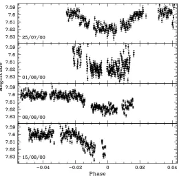
A prototype instrument was installed on La Palma from June - August
2000 [Kane et al., 2004] and observed the Pegasus field. The known transiting planet HD 209458 b was observed to transit as shown in Fig. 1.11 proving that the
instrument could detect transiting planets.
The final instruments are similar in design with f/1.8 200 mm telephoto lenses, 4 megapixel CCDs with 13.5µm pixels, and a wide spectral response (400 nm
- 700 nm) to maximise the light collected. Figure 1.12 shows the phase folded
lightcurve of the first WASP planet, WASP-1 b. WASP is ideal for detecting hot Jupiters as the large sky area observed maximises the chances of finding these
rare objects. The project has produced the lowest density planets detected from
the ground (WASP-31 b and WASP-57 b at 0.132 g cm−3 and 0.12 g cm−3 respec-tively), the hottest planets detected from the ground (WASP-33 b and WASP-12 b
discov-Figure 1.12: Phase folded lightcurve of WASP-1 b. Crosses denote 2004 season WASP photometry, and filled circles show the Volunteer Observatory light curve of 2006 October 1 [Collier Cameron et al., 2007b].
ery (WASP-17 b at 1.93+0−0..0521 RJ).3 Brown et al. [2011a] study WASP-18 b and WASP-19 b and constrain the stellar and planetary tidal quality factorsQ0s and Q0p
through Monte Carlo fitting and propose that WASP-19 b may have a remaining
lifetime of 0.0067+1−0..10730061 Gyr suggesting rapid infall. The large errorbars for this result are due to large uncertainties on the stellar age estimation.
The project excels at detecting hot Jupiters due to their large size and
rela-tively deep transit depth, but the project’s strengths are the large number of stel-lar targets observed and the brightness of the targets. WASP planets are often
good candidates for atmospheric studies as they transit frequently, typically orbit
bright host stars, and often have large atmospheric scale heights (WASP-17 b and WASP-39 b in particular). These hot Jupiters are rare [e.g. Howard et al., 2012]
but relatively easy to detect. By observing a large stellar sample, the population of
these unusual objects can be understood allowing WASP to lead the analysis of hot Jupiter populations, provided the selection effects can be understood (Chapters 2
and 3).
1.4.2 Kepler
The Kepler mission was designed to determine the frequency of Earth-sized planets
in and near the habitable zone of Sun-like stars [Borucki et al., 2010]. The other
scientific goals include determining the radius and semi-major axis distributions of the planets and to estimate and characterise the multi-planet systems [Borucki et al.,
2009]. By observing from space the mission is not hindered by observing through the
Earth’s atmosphere allowing for much higher precision measurements of the stellar
flux and detecting smaller transit depths than is possible from the ground. The
target precision was such that the transit of an Earth-sized planet around a 12th magnitude G2 star would be detected at 4σ [Borucki et al., 2010]. The spacecraft
was launched on March 6 2009 into an Earth-trailing orbit continuously observing
a sample of 150000 stars for transit events.
To date 136 confirmed or validated planets have been discovered, with over
3500 candidate planets awaiting validation. The planet candidate hosting stars
that are typically observed with Kepler are too faint to perform radial velocity analysis of, so statistical vetting is used to argue the validity of the planet candidates
detected. Planets are often validated through BLENDER estimation of the false
positive chance [Torres et al., 2004, 2005]. Multi-planet systems are often confirmed through dynamical estimation of the masses in the system based on orbital solutions
constrained by the observed transit timing variations (TTVs) where differences in
the mid-points of the transits allows the presence of another massive body in the system to be inferred. This method requires co-planarity of the systems which places
constraints on planetary migration methods.
The Kepler mission has found a wealth of interesting individual planets, from sub-Earth sized planets (e.g. Kepler-37 b, Kepler-62 c and Kepler-42 d) to the most
dense planet to date Kepler-68 c. The extremely high precision of the photometric measurements allows the detection of very small planets, especially around the later
type stars available in the Kepler field of view. Though the Kepler instrument
was designed to search for small planets, the project has detected Jupiter class planets with exquisite photometric quality (e.g. Kepler-12 b [Fortney et al., 2011],
Kepler-17 b [D´esert et al., 2011]). Example Kepler lightcurves for a hot Jupiter and
super Earth are shown in Fig 1.13. In the case of Kepler-17 b the starspots and high stellar rotation rate allow a limit to be placed on the orbital obliquity of<15◦.
Kepler has shown that multi-planet systems are common and are in stable
coplanar orbits [Lissauer et al., 2011]. The distribution of observed period ratios shows that the vast majority of candidate pairs are neither in or near low-order
mean motion resonances, though a non-negligible sample are, especially near the 2:1
resonance. Resonant orbits of multi-planet systems are thought to be an indicator of smooth disk migration, and the co-planarity supports this.
Kepler has discovered planets in binary star systems, both wide binaries and
close binaries where the planet orbits both stars. Kepler-16 b was discovered around an M1III detached binary. The orbital solution of the three body system allowed


![Figure 2.5: Initial test results for only varying the planetary radius of WASP-12 b.Black circles indicate tested values, the dashed vertical line represents the literatureradius value of 1.736±0.092 RJ [Chan et al., 2011], the grey region representing theuncertainty.](https://thumb-us.123doks.com/thumbv2/123dok_us/9614295.464180/76.595.188.455.110.313/initial-planetary-indicate-vertical-represents-literatureradius-representing-theuncertainty.webp)