MASTER THESIS
APPLIED
MATHEMATICS
C
HAIRM
ULTISCALEM
ODELING ANDS
IMULATIONDirect Numerical Simulation of Bubble-Wall Interactions
Author
S.R. Ephrati
s1422197
Supervisor
Prof.Dr.Ir. B.J. Geurts
Graduation committee
Prof.Dr.Ir. B.J. Geurts
Prof.Dr.-Ing. J. Fröhlich
Dr. M. Schlottbom
This master thesis concludes my graduation project and with it my time as a student. It closes off an enjoyable six years at the University of Twente during which I have left the lovely Friesland behind and have made the remote Enschede my home. Student life has allowed me to develop myself in a lot of ways to become the person I am today, to experience many exciting moments and activities, and to make many new friends with whom I have had a lot of fun over the years.
I would like to take this opportunity to thank several people. First of all I want to thank my supervisor prof. Geurts, who made it possible for me to go abroad during my internship and offered me this interesting subject to work on during my final year. During my final project I have often been amazed by the ability to untangle my thoughts and keep me busy for an entire week just by having a simple ten minute discussion.
I also want to thank prof. Fröhlich and Benjamin Krull for hosting me in Dresden and making me feel welcome in the Fluid Mechanics group. I have enjoyed the couple of months I spent in the group as well as the many discussions about serious and a little less serious subjects (mostly regarding cyclists and linguistic differences between German and Dutch). All in all, I look back at my time in Dresden with a very positive feeling.
I would also like to express my gratitude to Paolo Cifani, the developer of the TBFsolver. We have had quite some contact at the start of the project, when I had to learn how to use the pro-gram. Thank you for the quick responses to the (very) many e-mails I sent, and the time you have taken to explain me how to use the TBFsolver.
Needless to say I would like to thank my parents, without whom I would not have been able to study in the first place. You have invested a lot of time and effort in me, probably without even understanding what it actually is that I have been studying. Special thanks also go to my good friends David, Frank, Sander, Rico and Mike, with whom I have enjoyed many cups of coffee and many beers over the years.
The motion of a bubble impacting on a solid wall is studied numerically using the open-source code TBFsolver for the simulations of multiphase flows. This code employs Direct Numerical Simulation (DNS) using a volume of fluid (VOF) approach, and has already been tested for sit-uations involving a single bubble as well as a vast number of bubbles. An extensive study is performed for a single bubble hitting a wall head-on and under an angle of 45 degrees. Bubble movement and deformation suggest that the small-scale processes that occur during bubble-wall interactions are captured well by the solver. Geometric quantities along with the energy dissipation near the bubble are compared to an existing bubble collision model.
Preface i
Abstract iii
1 Introduction 1
1.1 Multiphase flows and the importance of DNS . . . 1
1.2 Goal and structure of this study . . . 1
1.3 Criteria for the comparison of multiphase flow solvers . . . 2
1.4 Variables and notation . . . 2
2 Description of the TBFsolver 3 3 Bubble-wall interactions 5 3.1 Introduction . . . 5
3.2 Recreating the case of Heitkam et al. . . 6
3.3 Testing the assumptions of Heitkam et al. . . 10
3.4 Results 45 degree case . . . 13
3.5 Results 0 degree case . . . 18
3.6 Concluding remarks . . . 21
4 Lubrication theory 23 4.1 Nondimensionalization of the Navier-Stokes equations . . . 23
4.2 Simplification of nondimensionalised Navier-Stokes equations . . . 25
4.3 Finding the lubrication pressure . . . 28
4.4 Lubrication pressure in one-dimension . . . 29
4.5 Application to explicitly defined interfaces . . . 32
4.6 Application to the case of Heitkam et al. . . 35
4.7 Application of lubrication theory to the TBFsolver . . . 39
4.8 Concluding remarks . . . 40
5 Conclusions 41 6 Discussion and recommendations 43 Bibliography 45 A Nomenclature 47 A.1 Variables and vectors . . . 47
1.1
Multiphase flows and the importance of DNS
This master thesis deals with numerical simulations of multiphase flows, where multiple fluid phases are present. These flows occur in many industrial situations and play an important role in many applications, such as vaporization and combustion of dense sprays, or heat exchangers and cooling systems in industrial plants. A good understanding of these flows can be crucial for safety reasons in applications as cooling systems. Multiphase flows also occur in natural situations or situations closer to everyday life. Think of the formation of rain drops or bubbles in carbonated soft drinks.
A typical example which is often considered is that of bubbles of air dispersed in liquid water. In this situation the continuous phase, the phase that occupies a connected region of space, is water, and the dispersed phase, which occupies disconnected regions of space, is air. The si-multaneous existence of multiple phases increases the complexity of the flow and introduces smaller time and length scales. For example, a thin liquid film remains between a bubble and an obstacle during an interaction, with a typical thickness many times smaller than the bubble radius.
Interactions between between bubbles and obstacles frequently occur in multiphase flows when a large number of bubbles is present. These obstacles can be other bubbles, or the walls of the container or channel in which the bubbles move. This emphasizes the relevance of having a ad-equate knowledge of how these interactions take place and what their influence is on the flow.
The presence of multiphase flows in many practical applications stresses the importance of having a good understanding of the behaviour of these flows and the processes that take place within them. It is for this purpose that numerical simulations are used. Numerical simulations allow for control over a lot of variables, which might not always be the case in practical exper-iments. However, numerical simulations are built on mathematical methods which are subject to errors and it is for this reason that one should properly assess the credibility of the results. One of the numerical methods used for simulating multiphase flows is direct numerical simu-lation (DNS). This method aims to computationally resolve the flow down to the smallest scales without the use of models to account for certain physical processes. Simply put, this means that a proper DNS of a multiphase flow yields the exact solution of the governing equations.
1.2
Goal and structure of this study
This study revolves around the TBFsolver, a program developed to simulate multiphase flows. The goal is to investigate bubble-wall interactions and compare the findings to existing collision models. The motivation for this is twofold. Firstly, extensively studying bubble-wall interac-tions with the TBFsolver grants new insights into these interacinterac-tions and how the solver deals with these situations. Secondly, the strengths and weaknesses of existing collision models can be identified by comparing the results to DNS data. This in turn might result in improvements for the methods and for identifying the range of application in which the models can be used.
from an existing collision model. A theoretical approach to bubble-wall interactions is consid-ered in section 4 by using lubrication theory and these results are subsequently compared to the data obtained from the TBFsolver. The thesis closes with the conclusions in section 5 and a discussion in section 6.
1.3
Criteria for the comparison of multiphase flow solvers
Several criteria are kept in mind when comparing the numerical methods, of which the most important ones are listed below.
• Stability
• Accuracy, which includes accurate flow computations and bubble deformations, and con-vergence rate of numerical solutions. both qualitatively and quantitatively
• Computational cost
Other points of interest are the effort required to add additional functionality to the solver and change the built-in functions and the ease with which relevant quantities can be calculated.
1.4
Variables and notation
Physical parameters are used throughout this thesis. These parameters can be viewed as if they are divided by the corresponding physical SI unit, therefore no units have been used in this report. This has been done because our interest lies not in the particular choice of physical parameters, but rather in the dimensionless numbers following from those parameters.
Vectors are denoted using bold characters. For example, we writeu = (u, v, w)to denote the velocity vector with componentsu, vandw. The reader is referred to appendix A for a list of variables and dimensionless numbers.
The TBFsolver is the numerical code with which the simulation data throughout this report is obtained. A brief description of the governing equations and numerical algorithm are pro-vided for completeness. The description closely follows along the lines of Cifani [6], for a full description the reader is referred to Cifani [6] and Cifani et al. [5].
Governing equations
The numerical technique used in the TBFsolver is the volume of fluid (VOF) method. The mathematical model for multiphase flows follows the one-fluid formulation, i.e., a single set of equations is solved on the entire domain and material properties and interfacial terms are accounted for using a marker function f. Each bubble is given a marker functionfi which
equals 1 in cells where the bubble fully occupies the cell, 0 where the fluid occupies the cell, and a value between 0 and 1 indicates that the cell contains a bubble interface. The value of the marker function is also referred to as the volume fraction. GivenN bubbles, the marker functions are advected via
∂fi
∂t +u· ∇fi= 0 fori= 1, . . . , N. (1)
The nondimensionalized incompressible Navier-Stokes equations and incompressible continu-ity equation are used to describe the flow:
ρ
∂u
∂t +∇ ·(uu)
=−∇p+ 1
Fr2ρˆg+
1
Re∇ ·(2µD) +
1
Weknδ(n) (2)
∇ ·u= 0 (3)
Hereuis the velocity,tis the time,pis the pressure,ρthe density,µthe viscosity,kis the cur-vature,ˆgis the normalized gravity vector,Dthe deformation tensor, andnis the normal vector to the interface. The dimensionless numbers are the Froude number Fr=U/√gL, the Reynolds number Re=U Lρ1/µ1, and the Weber number We=LU2ρ1/σ. HereLandU denote a charac-teristic length and a characcharac-teristic velocity, respectively. The subscript 1 denotes the continuous phase.
The Froude number is defined as the ratio between inertial forces and gravitational forces. The Reynolds number gives the ratio between inertial forces and viscous forces. A small Reynolds number indicates that viscous forces dominate and generally occurs in laminar flow, whereas a large Reynolds number characterizes turbulent flow. The Weber number is a measure of the importance of the inertia of the flow compared to the surface tension. Strong bubble deforma-tion is typical for high Weber numbers.
The density and viscosity at a certain point follow from the marker functions and the properties of the continuous and dispersed phases. For instance, a cell with volume fraction valuecwould have a density and a viscosity of
ρ=ρ1(1−c) +ρ2c, (4)
Discretization of surface tension and interface curvature
The continuous surface force (CSF) method [4] is used to model the surface tension term. This method replaces the delta functionδ(n)nby a smooth term, which is computationally easier but also suffers from spurious currents. These spurious currents are unphysical velocities gen-erated by the discretisation of the surface tension.
Reducing spurious currents can effectively be done by accurately computing the curvature of the interface [9]. The TBFsolver uses a height function method for this purpose. This method constructs a local height function from the volume fraction in the computational cells and dif-ferentiates this function to obtain the curvature. The reader is referred to Cummins et al. [7] for a detailed description of this method.
Spatial discretization
A three-dimensional Cartesian grid is used to discretize the domain. A uniform grid in all di-rections is chosen throughout this report. The TBFsolver currently offers both collocated and staggered arrangement of the variables. However, a staggered arrangement was the only avail-able option at the time at which most of the tests in this report were performed. The velocity components are then defined on the cell edges, the pressure and the volume fraction field are defined at the cell centers. This arrangement ensures a strong coupling between pressure and velocity [5].
The spatial discretization of the convective term in equation (2) is based on the finite volume approach. Additionally, the QUICK interpolation scheme [15] is implemented in the TBFsolver and has been used for the simulations in this report. This scheme avoids the presence of un-physical oscillations that occur for increasing Reynolds numbers [16]. A second order finite difference scheme is employed for the diffusive term.
Temporal discretization
A third-order Runge-Kutta scheme is used to discretize the convection and diffusion terms of the Navier-Stokes equations, a Crank-Nicolson scheme is employed for the surface tension term. The time integration follows a fractional step approach, in which each time step is com-posed of three stages ts. Here we have that s = 0 corresponds to time steptn and s = 3
corresponds to the new time steptn+1. The following actions are performed per stagets.
• The marker functions are advected and the bubble interface is reconstructed, yieldingfat
ts+1.
• A provisional velocityu∗ is obtained, based on the velocities of the previous stages and the material properties of the previous and the current time step.
• The pressure in the new time step is calculated by solving a Poisson equation, using the provisional velocity.
3.1
Introduction
It is very likely that bubbles interact with each other or with walls when considering a turbulent flow with a large number of bubbles. The bubble seems to be in contact with the obstacle during such interactions, though this is not the case. A thin liquid film, a ‘lamella’, remains inbetween the objects, which causes a bounce when the thickness remains above a certain threshold. Rup-ture of the film results in coalescence in the case of a bubble-bubble interaction [19]. In this section we will only consider bouncing as the outcome of the interactions, since bubble coales-cence is not included in the TBFsolver.
The presence of the liquid film between the bubble and the obstacle introduces small length scales into the flow. For example, bubble coalescence takes place when the thickness of the film reaches a molecular interaction range [20], which typically is of the order of102Å (10−8meter) [17]. Fully resolving these newly introduced length scales requires a very fine grid, which is practically infeasible even when simulating a single bubble. Hence it is desirable to introduce a model which captures the small-scale processes and eliminates the need for a very fine grid. This requires knowledge of the processes taking place during interactions in order to argue which of those processes can be neglected or approximated without severely deteriorating the quality of the solution.
The topic of this section is a rising bubble which at some point hits a wall. This problem is strongly related to the problem considered by Heitkam et al. [12]. This paper presents results of bubble-wall interactions using physical experiments as well as numerical experiments, and subsequently propose a collision model for small bubbles.
The first numerical experiment performed in this section considers three cases of a bubble in-teracting with a wall due to gravity and is similar to the physical experiment performed in the mentioned paper. This experiment demonstrates that a meaningful bubble-wall interaction is taking place at all and shows that the choice of parameters allows for a good comparison with the results of Heitkam et al.
The model of Heitkam et al. results in physical behaviour whilst requiring low computational effort. It is interesting to see how the physical model compares to results of simulations with the TBFsolver providing detailed resolutions of the bubble-wall interactions, and at which points the proposed model differs from the results of the TBFsolver. Moreover, the assumptions on which the model is based can be tested and possibly improved. This comparison is performed in the second numerical experiment, which consists of a detailed study of one of the cases of the first experiment.
3.2
Recreating the case of Heitkam et al.
Problem description and goal
The goal of this numerical experiment is to replicate the physical experiment performed in the reference paper. This has two main motivations. Firstly, it is important to know whether situ-ations such as those considered by Heitkam et al. can be recreated properly by the TBFsolver. Secondly, successfully recreating the physical experiment allows us to continue studying the case in more detail and to extensively test the proposed model. Recreating the physical exper-iment is not trivial, since not all required dimensionless variables are stated in the reference paper and the parameter choice influences the stability of the simulation.
Three different cases are simulated using the TBFsolver, with a set of parameters based on the information provided in the paper of Heitkam et al. The results are compared and subsequently a single set of parameters is chosen for further comparison in the next section.
Numerical setup
The initial configuration is shown in figure 1. This figure shows a two-dimensional slice of the domain parallel to thexy-plane.
The domain is a cuboid tank with a solid top and bottom, and periodic boundaries on the side. An inclined wall at the top of the domain is achieved by changing the direction of gravity, i.e. by changing the value ofα. The value ofαequals the angle the direction of gravity makes with they-axis, withα= 90◦corresponding to gravity being parallel to thex-axis.
The bubble is initially spherical with radiusR = 0.5and is placed such that the distance be-tween the center of mass of the bubble and the top wall equals11.3Rin the direction of gravity, equal to the initial position of the bubble in the numerical experiment performed in the refer-ence paper. This distance is denoted byLcin figure 1. The entire domain is a cube with a length
of12.8Rin each direction. A grid with 128 cells in each dimension is employed, corresponding to 10 grid cells per bubble radius. This is denoted byR/hin table 1 and the chosen grid is suffi-ciently fine to properly resolve the shape of a deforming bubble [6].
The parameters used for the cases are given in table 1. The density and viscosity ratios are equal to those of air and water, where water represents the continuous phase and air the dispersed phase. The Eötvös number and the Reynolds number are given in the reference paper, but the latter is an output parameter rather than an input parameter. For this reason the Galilei number is used, which can be determined a priori. This number represents how quickly the bubble will accelerate due to the density differences of the phases. The value of the Galilei number is varied throughout the test cases by varying the viscosities. The Eötvös number gives the ratio between gravitational forces and surface tension forces and serves as a measure of how easily a bubble deforms. A higher value of the Eötvös number indicates that the bubble is not easily deformed.
Table 1: Numerical simulation setup and material properties.
Test case R ρ1 ρ2 µ1 µ2 g σ R/h ∆t
R
12.8R
12
.
8
R
L
c
g
α
1 2
y
[image:15.595.187.380.98.294.2]x
Figure 1: Initial configuration. The bold numbers indicate the phases.
The following dimensionless numbers are used to describe the test cases.
• Density ratioρ1/ρ2;
• Viscosity ratioµ1/µ2;
• Eötvös numberEo = (ρ1−ρ2)gL2/σ;
• Galilei numberGa =ρ1 p
|ρ2/ρ1−1|gL3/µ1.
The characteristic lengthLis chosen as the bubble diameter. The values of these dimensionless numbers for the considered cases are given in table 2.
Table 2: Dimensionless numbers corresponding to the variables in table 1.
Test case ρ1/ρ2 µ1/µ2 Ga Eo
3.1 845 48 145 0.48
3.2 845 48 130 0.48
3.3 845 48 140 0.48
Quantities of interest
Several quantities of interest are used for verifying whether the obtained data is genuinely DNS data, in the sense of fully resolving all dynamically relevant scales, and for testing the assump-tions made by Heitkam et al. In the definiassump-tions belowΩ2(t) is the domain occupied by the dispersed phase a timet, with|Ω2|being the corresponding volume.
• Bubble movement
– Center of mass:x¯(t) =|Ω2|−1RΩ
2(t)xdx.
[image:15.595.206.388.487.537.2]i) u¯t(t) =|Ω2|−1RΩ
2(t)uxdx, the velocity tangent to the wall,
ii) u¯n(t) =|Ω2|−1RΩ
2(t)uydx, the velocity normal to the wall,
iii) u¯ = sin(α)¯ux+ cos(α)¯uy, the velocity parallel to the direction of gravity.
• Bubble deformation
– Bubble diameter: d(t) = (d1(t), d2(t), d3(t)), wheredi(t) = maxx,y∈Ω2(t)|xi −yi|,
i= 1,2,3.
– Contact area with the wall, expressed as the radiusRa of the circle with the same
area. The definition is discussed in section 3.3.
• Energy dissipation inside the fluid:ε= 2µ1
ρ1S
2
ij; S =
1
2 ∇u+∇u
T .
The center of mass is calculated as the averaged integral of the position over the volume occu-pied by the bubble. The bubble velocity is calculated similarly using the velocity rather than the position. Integration is performed numerically using the trapezoidal rule. The diameter essen-tially is the maximum distance occupied by the dispersed phase in each spatial dimension. We are especially interested in the diameter increase during the collision process, for comparison with the model of Heitkam et al.
Determining whether the flow is fully resolved is interpreted here based on the normal distance between the bubble and the wall. We assume that the flow between the bubble and the wall can be properly resolved as long as this distance equals four grid cells.
The bubble movement is of importance, if the corresponding quantities have not converged we can assume the overall solution has not converged. Moreover, the lamella thickness is consid-ered an important quantity, but properly measuring this quantity might not be possible because of it being smaller than the grid size.
The energy dissipation is calculated in multiple regions in the fluid, directly related to the bub-ble. The regions we consider are the entire fluid, the control volume and the fluid lamella, as shown in figure 2. The control volume is defined as the area between the bubble and the wall. Note that figure 2 exaggerates the thickness of the lamella for illustrational purposes; the actual lamella is many times thinner. Moreover, the control volume includes the lamella when the bubble is in the vicinity of the wall.
R
Lamella Control volume
Results
Figure 3 shows the bubble trajectories for the considered test cases. The trajectories are calcu-lated by following the center of mass during the simulation. The dashed lines represent the bounds given by the experimental data presented in the reference paper. The blue line is the result of the collision model of Heitkam et al., this data was taken directly from the paper. The experimental data consists of measurements at different points in time, which have been performed for multiple bubbles seperately. No trajectories have been reconstructed using this data, rather the entire set of measurements has been displayed. The experimental bounds have been deduced from this set by drawing upper and lower bounds which contain most of the measurements and suggest that that a single major bouncing event takes place.
Figure 3: Trajectories for the different cases compared to the data from Heitkam et al.
Interpretation of the bubble trajectories
Figure 3 shows that the results of the TBFsolver fit within the experimental bounds, as desired. In addition, it is clear that the results of the TBFsolver and the numerical results of Heitkam et al. differ strongly. The main cause is probably the rebound of the bubble after the initial contact with the wall. The simulation results from the TBFsolver suggest that a bouncing event takes place, whereas the numerical results of Heitkam et al. show the bubble interacting with the wall and sliding along the wall afterwards. Moreover, the initial rebound in the simulations of the TBFsolver results in several consecutive interactions with the wall, where each subsequent interaction yields a smaller bouncing event.
3.3
Testing the assumptions of Heitkam et al.
Problem description and goal
We have shown before that the experimental results of the case of Heitkam et al. can be recre-ated using the TBFsolver. The goal now becomes to test some of the assumptions made by Heitkam et al. by using grid refinement for several cases.
The original approach was to use simple, inexpensive test cases which progressively get phys-ically more relevant and harder to calculate. The idea behind this is that the fluid lamella that appears during a bubble-wall interaction is easier to fully resolve in non-physical test cases, so DNS data can be obtained. Results have shown that fully resolving this lamella with the TBFsolver is only possible when a situation without gravity is considered. However, these sit-uations differ too much from the physically relevant cases and are therefore not considered useful.
Instead, the applied approach makes use of one of the situations used in the previous sub-section. It is known that parts of the flow will not be properly resolved during a part of the bubble-wall interaction for this case. Nonetheless, the results can be compared for the parts of the simulation where the flow is fully resolved, i.e., where the smallest length scales of the flow are well resolved on the grid. Even though this means that no DNS data is obtained for the entire domain and the entire duration, we will still consider values of geometrical quantities of interest in order to test the assumptions made in the Heitkam paper.
Summarizing, by performing said simulations we hope to achieve the following goals.
• Obtain DNS data during the approach of the bubble to the wall and reliable data during the bubble-wall interaction.
• Use the data to find in which areas the simulation performed with the TBFsolver is not DNS and investigate how this influences the results of the simulations of the bubble-wall interaction.
• Use the obtained data to test and possibly improve the assumptions made in the reference paper.
Implementation of boundary conditions at the wall in the TBFsolver
The TBFsolver employs a contact-angle model to allow for physically relevant bubble-wall in-teractions [6]. This model is based on the work of Afkhami and Bussmann [2], and is briefly explained here for completeness.
The contact angle describes how the bubble interface should be reconstructed near the wall, more specifically, it describes towards which direction the interface normal should point for certain cells near the wall. The direction of the interface normal is uniquely determined by the contact angle in two-dimensional cases and is explained here. The idea for three dimensions is slightly more extensive but follows along the same lines.
The contact angle in two dimensions determines the interface normal as follows.
• A contact angle of90◦means that the interface normal and the wall normal are perpen-dicular to each other, and therefore the bubble makes contact with the wall at an angle of
90◦.
• A contact angle of180◦ indicates that the interface normal and the wall normal point directly towards eachother, which results in the presence of a film of fluid between the bubble and the wall.
As stated by Cifani [6], the choice of the contact angle only slightly affects the mean properties of the flow in turbulent channel bubbly flows, since it only affects the shape of the bubble in close proximity to the wall. However, a contact angle of180◦is implemented in the TBFsolver as a standard boundary condition choice for the volume fraction field to allow for physically relevant bubble-wall interactions. This is also the boundary condition which has been used throughout the simulations in this section.
Definition of the fluid lamella
A thin film of fluid remains between the bubble and the wall during bubble-wall interactions. This film is experimentally shown to be approximately 30 to 100 times smaller than the bubble radius for some instances [19]. It should be noted that these values are measured for smaller viscosity ratios than the case considered in this report, but still provide us with an estimate of the thickness. We therefore assume that the lamella is contained within the first layer of cells adjacent to the wall on the coarsest considered grid (R/h = 10) and the first refinement (R/h= 20).
Calculating the quantities of interest
An important quantity is the fluid lamella thickness. It is assumed that the interface near the wall is locally tangent to the wall, which means that the distance between the bubble and these cells is(1−c)∆xif the cell has a nonzero volume fractionc. This is also in agreement with the boundary condition employed by the TBFsolver, and is assumed to give a good approximation of the local lamella thickness. Furthermore, the volume fraction in each cell is readily available from the TBFsolver.
It is unclear how to calculate the other quantities of interest which are related to the fluid lamella exactly. However, approximations for these quantities can be made and the results on different grids can be compared.
There are two problems we need to overcome when calculating the quantities of interest related to the fluid lamella. Firstly, it is unclear at which distance from the wall the bubble should be considered in contact with the wall, since it is known that fluid is always present between the bubble and the wall. In addition, it is unknown which distance between the bubble and the wall should exactly be considered as the fluid lamella when calculating the dissipation. Sec-ondly, the flow in the fluid can not be calculated exactly in computational cells that contain the bubble interface. We elaborate on these points below.
we consider the bubble to be in contact with the wall, if the value of the volume fraction field is above a certain threshold value in a computational cell adjacent to the wall. We will denote this value bycth. Note that a volume fraction ofcthin a cell adjacent to the wall implies that the local distance between the bubble and the wall is(1−cth)∆x. Clearly, the contact area is dependent on the value ofcth and hence it is best to compare the results for multiple value of
cth.
When comparing the results on different grids, the value ofcthshould be chosen per grid such that it agrees with the grid refinement. For example, if on a certain grid the value ofcth is known, the value used on a grid with a coarsening of a factor two in the wall-normal direction is0.5 + 0.5cth. This idea is sketched in figure 4.
0.7
[image:20.595.216.416.233.350.2]0.85
Figure 4: The same distance between the bubble and the wall on different grids can be compared by using the right values of the volume fraction field. This example shows that a valuecth= 0.7 on the fine grid (left cell) corresponds to a value of0.85on the coarse grid (right cell).
A computational cell that contains the bubble interface is, by definition, partially filled with liquid and partially filled with gas. Hence the density and the viscosity in this cell are averaged based on the volume fraction field, as stated in equations (4) and (5). This causes the TBFsolver to regard the contents of this cell as a mixture of both phases when calculating the flow inside the cell. Thus it is impossible to find out how the flow behaves in each phase separately. Calcu-lating the dissipation in the fluid is therefore not trivial in cells that contain the interface. This becomes a problem when calculating the dissipation in the lamella. As stated before, the calculation of any quantity related to the lamella should be seen an approximation and for that reason the dissipation in the lamella is calculated considering multiple values of cth as the lamella. This grants an outline of the qualitative development of the dissipation inside the lamella over time, and provides an estimate for the actual dissipation taking place.
Assumptions in the Heitkam paper used for comparison
Not only is it interesting to compare the results of the TBFsolver with those of the model of Heitkam et al, the results can also be used to test some of the assumptions on which the model is built. The following assumptions in the reference paper can be tested against the data obtained with the TBFsolver:
• The fluid lamella thicknessh0. The proposed model usesh0 = q
3 8
p
• The relation between the bubble deformation ∆ and the contact area radius Ra. The
amount the sphere is deformed by the wall is represented by∆, given by
∆ =R−yc+h0. (6)
Note thatyc denotes they-coordinate of the center of mass of the bubble and equals the
minimal distance between wall and the center of mass and the bubble. The used relation between∆andRais
Ra
R =−30.0 +
r
900.0 + 0.424∆
R. (7)
• Energy dissipation in the fluid lamella. The model proposes thath0 remains constant throughout the collision process, which results in no dissipation inside the lamella but only near its rim.
Grid refinement study
We consider two cases of bubble-wall interactions. The first one is as performed by Heitkam et al., where the bubble approaches the wall under and angle of 45 degrees. The second case considers the same material properties but the bubble approaches the wall head-on. The di-mensionless numbers for these cases are given in table 3, these are the same parameters as used for test case 4.1, displayed in table 1. A1283grid and a2563grid are employed for both cases, a finer grid was not possible due to time limitations.
Table 3: Dimensionless numbers for case of Heitkam et al.
ρ1/ρ2 µ1/µ2 Ga Eo
845 48 145 0.48
3.4
Results 45 degree case
Figure 5: Bubble trajectory.
Figure 6:y-center of mass over time.
Figure 7: Velocity normal to the wall. Figure 8: Velocity tangential to the wall.
Comparison with the model assumptions
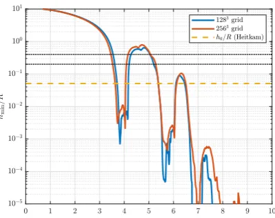
Figure 9 shows the minimal distance between the bubble and the wall. The dotted black lines are four times the grid sizes for both considered grids, the dashed yellow line represents the lamella thickness as expected from the Heitkam paper based on the bubble Reynolds number obtained from the TBFsolver. It is notable that the results of the TBFsolver on both grids show very little difference until the minimum distance is less than 0.5% of the bubble radius. The minimum thickness at this point exhibits relatively large fluctuations, which might be due to numerical inaccuracies. These observations lead us to conclude that the lamella thickness is not constant throughout the collision process. The variable lamella thickness in turn implies that energy dissipation does take place in the lamella.
[image:22.595.330.522.294.449.2]on the fine grid results in larger velocity gradients than on the coarse grid, which in turn yield a larger energy dissipation.
Figure 11 provides the energy dissipation in the control volume over time. The results on the used grids show the same developments. Approximately two-thirds of the overall dissipation in the fluid is taking place in the control volume during the initial contact. The remainder likely takes place in the wake of the bubble, which becomes more apparent after the initial contact when the wake starts to interact with the wall.
Figure 9: Minimum distance between the bubble and the wall.
Figure 10: Energy dissipation in the entire fluid region.
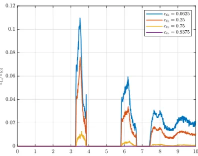
The energy dissipation in the lamella for the2563grid is given in figure 12. Even though it is not clear at which value ofcththe lamella is defined, it becomes clear from the figure that a sig-nificant fraction of the energy dissipation takes places between the bubble and the wall. This is likely caused by the sharp velocity gradient near the wall due to the no-slip boundart condition at the wall. The decrease of the dissipation in the lamella during the second contact with the wall is caused by the decrease of the wall-normal velocity compared to the initial contact.
Figure 11: Energy dissipation in the control volume as a fraction of the total dissipation.
Figure 12: Energy dissipation in the lamella as a fraction of the total dissipation on the2563 grid, for different values ofcth.
0 0.5 1 1.5 2 2.5 3 3.5 4 y/R
4.5 5 5.5 6 6.5 7 7.5 8
x/R
(a)t= 3.2
0 0.5 1 1.5 2 2.5 3 3.5 4 y/R
4.5 5 5.5 6 6.5 7 7.5 8
x/R
(b)t= 3.4
0 0.5 1 1.5 2 2.5 3 3.5 4 y/R
4.5 5 5.5 6 6.5 7 7.5 8
x/R
(c)t= 3.6
0 0.5 1 1.5 2 2.5 3 3.5 4 y/R
4.5 5 5.5 6 6.5 7 7.5 8
x/R
(d)t= 3.8
0 0.5 1 1.5 2 2.5 3 3.5 4 y/R
4.5 5 5.5 6 6.5 7 7.5 8
x/R
(e)t= 4.0
0 0.5 1 1.5 2 2.5 3 3.5 4 y /R
4.5 5 5.5 6 6.5 7 7.5 8
x/R 0 0.5 1 1.5 2 2.5 3
[image:24.595.327.526.98.255.2](f)t= 4.2
Figure 13: Energy dissipation in the vicinity of the bubble at different times on the1283grid. Note that the bubble has been translated to the center of the domain to obtain a clearer picture. The values range from 0 (blue) to 3 (red), values beyond this range are clipped.
0 0.5 1 1.5 2 2.5 3 3.5 4 y /R
4.5 5 5.5 6 6.5 7 7.5 8
x/R
(a)t= 3.2
0 0.5 1 1.5 2 2.5 3 3.5 4 y /R
4.5 5 5.5 6 6.5 7 7.5 8
x/R
(b)t= 3.4
0 0.5 1 1.5 2 2.5 3 3.5 4 y /R
4.5 5 5.5 6 6.5 7 7.5 8
x/R
(c)t= 3.6
0 0.5 1 1.5 2 2.5 3 3.5 4 y /R
4.5 5 5.5 6 6.5 7 7.5 8
x/R
(d)t= 3.8
0 0.5 1 1.5 2 2.5 3 3.5 4 y /R
4.5 5 5.5 6 6.5 7 7.5 8
x/R
(e)t= 4.0
0 0.5 1 1.5 2 2.5 3 3.5 4 y /R
4.5 5 5.5 6 6.5 7 7.5 8
x/R 0 0.5 1 1.5 2 2.5 3
(f)t= 4.2
Figure 14: Energy dissipation in the vicinity of the bubble at different times on the2563grid. The values range from 0 (blue) to 3 (red), values beyond this range are clipped.
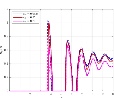
The contact areaRa with the wall over time is shown in figure 15, where several values ofcth are considered. The dashed lines represent the contact area based on the corresponding value ofcth on the coarse grid. The different values ofcth yield the same behaviour, with a slight increase of the amplitude ofRafor smaller values ofcth.
[image:24.595.110.307.100.255.2]reference paper. The proposed relation between∆andRais given by the dashed yellow line,
which clearly does not agree with the results from the TBFsolver. The relation between the vari-ables can be approximated by a square root function such asRa/R= 1.25
p
∆/R, depicted by the dashed purple line. This function is chosen for illustrational purposes and is not assumed to be the best approximating function.
It is unclear the cause is of the discrepancy between the prediction of Heitkam et al. of the relation between∆ andRa and the actual results. It seems as if the cause is a scaling issue.
[image:25.595.291.487.222.380.2]However, this should not be the case since equation (7) gives the relation between the nondi-mensionalized quantities∆/RaandRa/R.
Figure 15: Contact area radiusRafor different
values ofcth. The dashed lines represent the corresponding values ofcthon the1283grid.
[image:25.595.71.270.223.379.2]3.5
Results 0 degree case
[image:26.595.326.524.175.330.2]The development of the center of mass and the velocity of the bubble is shown in figures 17 and 18. Similar to the results of the 45 degree case, the bubble rises slightly faster on the fine grid than on the coarse grid.
Figure 17:y-center of mass over time. Figure 18: Velocity normal to the wall.
Comparison with the model assumptions
Figure 19 shows that the minimum distance between the bubble and the wall shows similar behaviour on both grids. The minimum distance during the collision process becomes smaller as the bubble Reynolds at the initial moment of the collision decreases. This is also observed when comparing these results to those of the 45 degree case (figure 9); the latter shows shows a smaller minimum distance at the first bubble-wall interaction.
A cross-section of the bubble shape near the wall is shown in figure 20. Note that the distance from the wall is expressed in the grid size of the2563grid in this figure, as to clearly show the dimpled shape of the lamella and the change over time.
The differences in the total dissipation on both grids are best seen in the peaks that occur when the bubble hits the wall, as shown in figure 21. The dissipation before the initial collision is equal to that of the 45 degree case, which is to be expected since the bubble moves freely and at the same velocity this period. The peak in the energy dissipation is between almost twice as large compared to the 45 degree case. This is caused by the larger approach velocity of the bubble, which results in larger fluid displacement in the lamella, which in turn yields a larger energy dissipation rate during the collision.
This effect can also be observed in figures 23 and 24, which both show higher peaks during the initial collision than their 45 degree counterparts.
[image:26.595.112.305.175.330.2]Figure 19: Minimum distance between the bubble and the wall.
[image:27.595.74.274.98.256.2]Figure 20: Shape of the bubble near the wall at different times. The dashed lines represent the results of1283 grid, the solid lines repre-sent those of the2563grid.
Figure 21: Energy dissipation in the entire fluid region.
Figure 22: Energy dissipation in the lamella plotted againstcthat fixed times.
Figure 23: Energy dissipation in the control volume as a fraction of the total dissipation.
Figure 24: Energy dissipation in the lamella as a fraction of the total dissipation on the2563 grid, for different values ofcth.
0 0.5 1 1.5 2 2.5 3 3.5 4 y /R
4.5 5 5.5 6 6.5 7 7.5 8
x/R
(a)t= 3.2
0 0.5 1 1.5 2 2.5 3 3.5 4 y /R
4.5 5 5.5 6 6.5 7 7.5 8
x/R
(b)t= 3.4
0 0.5 1 1.5 2 2.5 3 3.5 4 y /R
4.5 5 5.5 6 6.5 7 7.5 8
x/R
(c)t= 3.6
0 0.5 1 1.5 2 2.5 3 3.5 4 y /R
4.5 5 5.5 6 6.5 7 7.5 8
x/R
(d)t= 3.8
0 0.5 1 1.5 2 2.5 3 3.5 4 y /R
4.5 5 5.5 6 6.5 7 7.5 8
x/R
(e)t= 4.0
0 0.5 1 1.5 2 2.5 3 3.5 4 y /R
4.5 5 5.5 6 6.5 7 7.5 8
x/R 0 0.5 1 1.5 2 2.5 3
(f)t= 4.2
Figure 25: Energy dissipation in the vicinity of the bubble at different times on the1283grid. The values range from 0 (blue) to 3 (red), values beyond this range are clipped.
0 0.5 1 1.5 2 2.5 3 3.5 4 y /R
4.5 5 5.5 6 6.5 7 7.5 8
x/R
(a)t= 3.2
0 0.5 1 1.5 2 2.5 3 3.5 4 y /R
4.5 5 5.5 6 6.5 7 7.5 8
x/R
(b)t= 3.4
0 0.5 1 1.5 2 2.5 3 3.5 4 y /R
4.5 5 5.5 6 6.5 7 7.5 8
x/R
(c)t= 3.6
0 0.5 1 1.5 2 2.5 3 3.5 4 y /R
4.5 5 5.5 6 6.5 7 7.5 8
x/R
(d)t= 3.8
0 0.5 1 1.5 2 2.5 3 3.5 4 y /R
4.5 5 5.5 6 6.5 7 7.5 8
x/R
(e)t= 4.0
0 0.5 1 1.5 2 2.5 3 3.5 4 y /R
4.5 5 5.5 6 6.5 7 7.5 8
x/R 0 0.5 1 1.5 2 2.5 3
(f)t= 4.2
Figure 26: Energy dissipation in the vicinity of the bubble at different times on the2563grid. The values range from 0 (blue) to 3 (red), values beyond this range are clipped.
The contact area with the wall for different values ofcth is shown in figure 27. The obtained values on the different grids are in good agreement, especially compared to the 45 degree case. It is assumed that the disagreement in the 45 degree case is caused by the tangential movement of the bubble, which results in a larger grid dependency.
As with the 45 degree case, the proposed relation betweenRaand∆does not at all agree with
the data obtained from the TBFsolver. This is depicted in figure 28. The line given byRa/R=
the results.
Figure 27: Contact area radiusRafor different
values ofcth. The dashed lines represent the corresponding values ofcthon the1283grid.
Figure 28: Relation between the contact area
Ra/Rand the deformation∆/R.
3.6
Concluding remarks
In this section several tests regarding bubble-wall interactions are performed. The parameters in these test were specifically chosen such that the results could be compared to those in made for the model proposed by Heitkam et al. and some of the assumptions could be tested.
With the obtained data of the TBFsolver, we found the following results:
• The bubble movement and velocity on the coarse and fine grids were in strong agreement, even after the initial bubble-wall interaction.
• The minimum distance between the bubble and the wall showed the same behaviour on the coarse and the fine grids, even for values smaller than the grid size. Moreover, the value of the minimum distance during the collision becomes smaller for small normal bubble velocity.
• The energy dissipation in the fluid significantly increases during the bubble-wall inter-action. This effect is more pronounced for the 0 degree case than for the 45 degree case. The majority of the dissipation during the collision takes place in the control volume as defined earlier.
Regarding the assumptions made by Heitkam et al., we conclude the following:
• The lamella thickness is not constant during the collision. The average thickness is not determined, since it is unclear at what point the space between the bubble and the wall is actually considered as the lamella. However, the minimum distance between the bubble and the wall is not constant during the collision process.
[image:29.595.290.488.122.281.2]take place in the lamella for the 45 degree case, and up to twenty five percent for the 0 degree case.
The fluid film between the bubble and the wall possesses a useful property in the asymptotic aspect ratio between the wall-normal and the wall-tangential length scales. The difference in magnitude between these scales can be exploited to obtain an approximation of the Navier-Stokes equations, where viscosity is dominant [14]. The flow inside the fluid lamella can be reconstructed from these viscous flow equations. Lubrication theory describes the mathematics and analysis behind this approximation. Essential in this field is the Reynolds equation, which provides an expression for the pressure distribution.
Lubrication theory is traditionally used in many applications within mechanical engineering and is sometimes used for biomedical purposes as well. An example for the latter is the mod-eling of human joints, such as ankle joints [21]. Applications in mechanical engineering usually include lubrication for bearings. Oftentimes fixed shapes such as solid spheres (Davis et al. [8], Gu et al. [11], Goddard et al. [10]) or cylinders [22] are used, or the effects of surface roughness are included [3]. More general forms such as stated by Kundu et al. [14] often assume the flow is contained within two (nearly) parallel surfaces, which implies a negligible curvature. Simu-lation results in section 3 show that the curvature of the bubble interface at the lamella is clearly visible on the length scales of the lamella thickness and can therefore not be neglected.
This section deals with the derivation of the lubrication equations and the application of these equations to a bubble-wall interaction. This application requires the inclusion of the curvature. The Navier-Stokes equations are first simplified using the asymptotic aspect ratio of the length scales. Expressions for the velocity field are subsequently obtained, which in turn are used to achieve a description of the pressure distribution in the form of the Reynolds equation. The flow in the lamella can then be reconstructed by using a numerical approximation of the solu-tion to the Reynolds equasolu-tion.
This section is structured as follows. Nondimensionalization and simplification of the Navier-Stokes equations is described in sections 4.1 and 4.2, respectively. The general problem of find-ing the lubrication pressure is discussed in section 4.3 and a method for findfind-ing this pressure in a one-dimensional case is presented in section 4.4. This method is applied to explicitly defined bubble interfaces in section 4.5, to provide an example of a reconstructed flow for a given bub-ble interface. Subsequently, lubrication theory is applied to the results obtained in the previous section, this is shown in section 4.6. The possibilities of implementing lubrication theory in the TBFsolver are discussed in section 4.7. Concluding remarks are collected in section 4.8.
4.1
Nondimensionalization of the Navier-Stokes equations
Equations and scalings
The continuity equation and Navier-Stokes equations for incrompressible flows form the start-ing point for the analysis. These equations are given by
∇ ·u= 0, (8)
ρ
∂u
∂t +u· ∇u
=−∇p+µ∇2u+ρg.
We fully write down these equations, because the scalings are dependent on the direction under consideration: ∂u ∂x+ ∂v ∂y + ∂w
∂z = 0, (10)
ρ
∂u
∂t +u
∂u
∂x+v
∂u
∂y +w
∂u ∂z
=−∂p
∂x +µ
∂2u
∂x2 +
∂2u
∂y2 +
∂2u
∂z2
, (11)
ρ
∂v
∂t +u
∂v
∂x+v
∂v
∂y +w
∂v ∂z
=−∂p
∂y +µ
∂2v
∂x2+
∂2v
∂y2 +
∂2v
∂z2
, (12)
ρ
∂w
∂t +u
∂w
∂x +v
∂w
∂y +w
∂w ∂z
=−∂p
∂z +µ
∂2w
∂x2 +
∂2w
∂y2 +
∂2w
∂z2
. (13)
Using the scalings
x=Rx,˜ y=Ry,˜ z=H0z,˜
u=Uu,˜ v=U˜v, w=Ww,˜
∇=R∇˜, t= (R/U)˜t, p= (µU R/H02)˜p.
HereRis the bubble radius,H0 is the distance between the bubble interface and the wall. U denotes the flow velocity tangent to the wall, whereasW denotes the flow velocity normal to the wall. We omit the tildes from now on.
R
H0
x
z y
Figure 29: Sketch of the geometry.
Nondimensional form
Starting with the continuity equation, we obtain
U R ∂u ∂x + ∂v ∂y + W H0 ∂w
∂z = 0. (14)
Adding a term(U/R)∂w/∂zallows us to substitute equation (10) into (14). Subsequently sub-tracting the same term to keep the equation correct yieldsU =W R
H0, this is based on Manica
Using the film Reynolds numberRef = (ρH0W)/µwe obtain the nondimensionalized Navier-Stokes equations, given by
Ref
∂u
∂t +u
∂u
∂x+v
∂u
∂y +w
∂u ∂z
=−∂p
∂x +
H2
0
R2
∂2u
∂x2 +
∂2u
∂y2
+∂
2u
∂z2, (15)
Ref
∂v
∂t +u
∂v
∂x +v
∂v
∂y +w
∂v ∂z
=−∂p
∂y +
H02
R2
∂2v
∂x2+
∂2v
∂y2
+∂
2v
∂z2, (16)
Ref
∂w
∂t +u
∂w
∂x +v
∂w
∂y +w
∂w ∂z
=−R
2 H2 0 ∂p ∂z + H2 0 R2
∂2w
∂x2 +
∂2w
∂y2
+∂
2w
∂z2. (17)
4.2
Simplification of nondimensionalised Navier-Stokes equations
We are only interested in the situation where the bubble is near the wall, that is, whenH0/Ris small. Neglecting the termsH0/Ryields
Ref
∂u
∂t +u
∂u
∂x+v
∂u
∂y +w
∂u ∂z
=−∂p
∂x+
∂2u
∂z2, (18)
Ref
∂v
∂t +u
∂v
∂x +v
∂v
∂y +w
∂v ∂z
=−∂p
∂y+
∂2v
∂z2, (19)
∂p
∂z = 0. (20)
Recall thatRef =ρW H0/µandU H0=W Rand thereforeRefis small too, which in turn results
in
∂p
∂x =
∂2u
∂z2, (21)
∂p
∂y =
∂2v
∂z2, (22)
∂p
∂z = 0. (23)
All variables up to this point have been scaled, scaling back to the original variables gives us the following equations. Keep in mind that these involve the ‘physical’ variables:
∂p
∂x =µ
∂2u
∂z2, (24)
∂p
∂y =µ
∂2v
∂z2, (25)
∂p
∂z = 0. (26)
Flow inside the fluid film
Assume a bubble-wall interaction, with velocityug = (ug, vg, wg)at the bubble interface. We
distance between the bubble and the wall at(x, y), where we takez= 0at the wall. Integrating the equations above and applying the boundary conditions gives us
u(x, y, z) = 1
2µ ∂p
∂x z
2
−h(x, y)z
+ ug
h(x, y)z, (27)
v(x, y, z) = 1
2µ ∂p
∂y z
2−h(x, y)z + vg
h(x, y)z. (28)
The expression forwfollows from equations (27) and (28) and the continuity equation. For this reason the desired partial derivatives ofuandvare calculated as
∂u
∂x =
1 2µ
∂2p
∂x2 z
2−hz
− 1
2µ ∂p ∂x
∂h
∂xz−
∂h ∂x
ug
h2z, (29)
∂v
∂y =
1 2µ
∂2p
∂y2 z
2−hz
− 1
2µ ∂p ∂y
∂h
∂yz−
∂h ∂y
vg
h2z. (30)
Inserting these results into the continuity equation yields an expression for∂w/∂z. Integrating overzand applying the boundary conditionw|z=0= 0gives
w(x, y, z) =− 1
6µ
∂2p
∂x2 +
∂2p
∂y2
z3+ 1
4µ ∂ ∂x h∂p ∂x + ∂ ∂y h∂p ∂y z2 +1 2 ∂h ∂x ug
h2 +
∂h ∂y
vg
h2
z2. (31)
Fluid film evolution and wall-normal velocity in the case of negligible curvature
Equation (31) can be simplified when we assume the local fluid film thickness variation is small. This assumption means∂h/∂xand∂h/∂yare small, i.e., that the curvature of the bubble inter-face is small, which reduces the equation to
w(x, y, z) =− 1
6µ
∂2p
∂x2 +
∂2p
∂y2
z3+ h
4µ
∂2p
∂x2 +
∂2p
∂y2
z2. (32)
Applying the boundary conditionw|z=h=∂h/∂tgives
∂h
∂t =
h3
12µ
∂2p
∂x2 +
∂2p
∂y2
. (33)
Equation (33) allows us to express the wall-normal velocity in terms of the approach speed of the bubble. For this purpose we defineα(x, y, z) :=z/h(x, y), which will simply denoted byα, and write
w(α) = h
3
12µ
∂2p
∂x2 3α
2−2α3 = ∂h
∂t 3α
2−2α3
. (34)
This expression agrees with the boundary conditionw|z=h/2=d(h/2)/dt[23].
Fluid film evolution and wall-normal velocity
in the area near the wall. The change of volume occupied by the bubble can be expressed by the movement of the interface,∂h/∂t. The change of volume occupied by the fluid equals the outflow over the boundaries of the domain. This is mathematically expressed as
Z
x
Z
y
∂h
∂t dydx+
Z x Z y Z z ∂u ∂x+ ∂v
∂ydzdydx= 0, (35)
where the last volume integral resulted from the divergence theorem. In turn, this yields
∂h
∂t +
Z h(x,y) 0
∂u
∂xdz+
Z h(x,y) 0
∂v
∂ydz= 0. (36)
The two integrals can be rewritten using Leibniz’s rule:
Z b(x)
a(x)
∂
∂xf(x, t)dt=
d dx
Z b(x)
a(x)
f(x, t)dt
!
−f(x, b(x))· d
dxb(x) +f(x, a(x))·
d
dxa(x), (37)
after which we obtain
∂h
∂t +
∂ ∂x
Z h(x,y) 0
udz
! + ∂
∂y
Z h(x,y) 0
vdz
!
−ug
∂h
∂x −vg
∂h
∂y = 0. (38)
The integrals can be evaluated by simply using the expressions for u, equation (27), and v, equation (28), as found before:
Z h(x,y) 0
udz=− 1
12µ ∂p
∂xh(x, y)
3+1
2ugh(x, y), (39) Z h(x,y)
0
vdz=− 1
12µ ∂p
∂yh(x, y)
3+1
2vgh(x, y). (40)
Now the derivatives of these integrals are calculated and are given by
∂ ∂x
Z h(x,y) 0
udz=− 1
12µ
∂2p
∂x2h(x, y)
3+ 3∂p
∂xh(x, y)
2∂h
∂x
+1
2ug
∂h
∂x, (41)
∂ ∂y
Z h(x,y) 0
vdz=− 1
12µ
∂2p
∂y2h(x, y)
3+ 3∂p
∂yh(x, y)
2∂h
∂y
+1
2vg
∂h
∂y. (42)
We substitute these terms into (38) and rewrite the formulation to obtain a partial differential equation forh. Note thath(x, y)is simply written ashfor the sake of readability. The equation is given by
∂h ∂t + ∂h ∂x − 1 4µ ∂p ∂xh
2−1 2ug
+∂h ∂y − 1 4µ ∂p ∂yh
2−1 2vg
− h
3
12µ
∂2p
∂x2 +
∂2p
∂y2
= 0. (43)
When ∂h
∂t =wg, which is the case when the approach volume of the interface equals the
wall-normal velocity of the bubble, the Reynolds equation for constant density is obtained:
∂ ∂x h3 12µ ∂p ∂x + ∂ ∂y h3 12µ ∂p ∂y
=wg−
ug 2 ∂h ∂x − vg 2 ∂h
4.3
Finding the lubrication pressure
Finding the pressure in the gap between the bubble and the wall, the lubrication pressure, is the main problem of interest. This pressure can be used to either find the velocity profile in the gap using equations (27), (28) and (32), or to derive a certain resistance force that acts on the interface of the bubble similar to Zhang and Law [23].
Assume∂h/∂tand hare known. Then either the Poisson equation (33) can be solved for p
when the curvature is assumed to be small, or a solution to the Reynolds equation (44) can be found when the curvature is to be included. The advantage of using the Poisson equation (33) is that finding an analytic solution might be easier. However, neglecting the curvature effects only leads to accurate solutions in a limited number of situations.
Below it is argued that the Reynolds equation should be used for finding the pressure in the gap. Solving this equation can be done using regular methods for solving discrete Poisson equations, such as multigrid methods or methods involving the fast Fourier transform.
Domain and boundary conditions
The natural question that arises is what boundary conditions should be applied for the pressure. This depends on the domain in which the equation is solved. A pressure difference between the bubble and the liquid exists when the curvature of the interface is nonzero, as stated by the Young-Laplace equation. It would therefore be sensible to define a rectangular or square area around the bubble where the equation should be solved. A rectangular shape matches the spatial discretization used in the TBFsolver and can be chosen such that it encompasses all cells near the boundary for which0< c <1for the volume fraction.
The edges of the rectangular domain could consist of cells with a small value ofc, i.e., the value ofhis relatively large in these cells. This results in a small value of the lubrication pressure. In other words, at the edges of the domain it can be assumed thatp = 0. This choice coincides with that of Skotheim and Mahadevan [22].
Incorporatingug
Since we are interested in the velocity of the bubble interface inx,y, andzdirections, it would be logical to use the change in the volume fraction field for this case rather than the velocity field. Moreover, the volume fraction field is advected before the velocity in the current time step is calculated and the advected volume fraction field is used for calculating the velocity. An intuitive approach would be to defineugbased on the change of the center of mass of the
bubble. This approach basically states that∂h/∂tcan be replaced bywg, which turns equation
4.4
Lubrication pressure in one-dimension
We will now consider equation (44) reduced to one dimension with no movement tangential to the wall. After fully writing the derivative we obtain
h3
12µ
d2p
dx2 + 1 4µ
dh
dxh
2dp
dx =wg. (45)
For now it is assumed that the wall-normal velocity is equal for the entire bubble, which means
wgis independent ofx.
Analytic solution
When we definef(x) := 12h3µ andg(x) := wg
f(x), the equation as shown below is obtained. The notation of ddx is replaced by a prime0for readability, yielding
p00(x) +f
0(x)
f(x)p
0(x) =g(x).
(46)
From this point the following method for solving nonhomogeneous second order differential equations with non-constant coefficients is employed.
1. Substituteq(x)forp0(x)to obtain a first order differential equation.
2. Calculate the integrating factorγ(x) = expRff0((xx))dx. 3. Calculateq(x) =
Rγ(x)g(x)
dx γ(x) . 4. Integrateq(x)to obtainp(x) =R
q(x)dx.
Applying step 1 is straightforward and is not explicitly shown. The derivation ofγ(x)for step 2 yields
γ(x) = exp
Z f0(x)
f(x) dx
= exp
3
Z h0(x)
h(x) dx
= exp (3 [log(h(x)) + ˜c1]) =c1h3(x), (47)
wherec1is a constant. Recall thatg(x) =wg/f(x) = 12wgµ/h3(x)and therefore we obtainq(x)
as
q(x) =
R
γ(x)g(x)dx
γ(x) =
R
12c1wgµdx
c1h3(x)
= 12wgµx+ ˜c2
h3(x) . (48)
Finally, the pressure results from applying step 4,
p(x) =
Z
q(x)dx= 12wgµ
Z x+c 2
h3(x) dx. (49)
Unfortunately,h(x)is usually not known and if it is known, the termh3(x)would likely be very complex and impractical to work with. Equation (49) does provide some information about the pressure distribution in the one-dimensional case, namely:
• The pressure scales linearly with the approach speedwgand the viscosityµ.
Numerical method
Since the analytic solution can generally not be further evaluated than the form in (49), a nu-merical solution is used to investigate the behaviour of the function.
The domain on which the function is solved is[0,1]. The problem can be seen as axisymmetrical when the boundary conditions ofpandhare chosen properly. For this reason the left boundary, atx= 0, requiresp0(x) = 0andh0(x) = 0, which corresponds tox= 0being the radial center of the bubble interface. The lubrication pressure is assumed to be zero atx= 1, which is the case when the distance between the bubble and the wall is large.
A Gauss-Seidel solver is used to iteratively approximate equation (45). The domain is divided intoN intervals, withN+ 1interval boundaries at which the pressure will be calculated. The distance between the bubble and the wallh(x)and the spatial derivatives ofh(x)andp(x)are also defined on the interval boundaries. The derivatives are calculated using a standard central finite difference scheme.
Given the approximated solution at iterationkand at interval boundaries 1 toi−1, the solution at iterationk+ 1at interval boundaryican be calculated. Subsequently the solution at iteration
k+ 1is calculated at interval boundaryi+ 1, and so on until a solution has been calculated on the entire domain at iterationk+ 1. Applying this algorithm for the entire domain is called a sweep. Note that the superscriptskandk+1denote the iteration number, the other superscripts denote a power. The scheme is given by
fik= 12µwg
h3
i
−3
dh
dx
i
dp
dx
i
1
hi
, (50)
Lpki = p
k
i+1−2pki +p k+1
i−1
(∆x)2 , (51)
rik=fik−Lpki, (52)
dki = −(∆x)
2rk i
2 , (53)
pki+1=pki +dki. (54)
In order to properly incorporate the boundary conditionp(1) = 0, the interface shapeh(x)is de-fined using the desired shape forx≤xs. Here0< xs<1has a chosen value. Using a Dirichlet
boundary condition rather than a Neumann boundary condition on the right boundary is also desirable since applying the latter on both boundaries results in a non-unique solution. This is the consequence of the termc2in the integral in equation (49). The actual value of the pressure at the right boundary is dependent on the ambient pressure, but can be assumed to be zero without loss of generality.
An ellipsoidal shape is chosen forx > xsash(x)should be large at the right boundary. This
shape is desirable since the value ofh(1)can the be varied easily and an appropriate choice of
h(x)will lead to a continuous derivativeh0(x).
The numerical scheme (50-54) suffers from instabilities when curvature is present in the in-terface shape andnx is not sufficiently large at the same time. This is most likely caused by
inaccurate values ofh0(x)whenn
xis small, since no instabilities occur whenh(x)is constant.
In general, no instabilities have been found whennx≥100.
The introduction ofxsgrants us the opportunity to circumvent this problem. By definingh(x)
and choosingxssuch that the desired shape is obtained within the interval[0, xs]makes it
Validation of the numerical method
The numerical scheme (50-54) is validated by comparing the outcomes to the analytic solution (49). For this purpose we takeh(x) =hminconstant over the entire domain and fixµat1and
wgat−1, the latter means an approach velocity of 1. The pressure is then easily calculated and
after applying the boundary conditionsp0(0) = 0andp(1) = 0becomesp(x) = 6(1−x2)/h3 min.
The domain is divided into 150 equally sized intervals for this particular case and a total of
2.5×10⁵Gauss-Seidel sweeps are performed for each value ofh
[image:39.595.98.466.278.417.2]min. The results usinghmin= 1 are shown in figure 30. It clearly shows that the numerically calculcated pressure distribution approximates the analytical solution well, and consequently the derivative of the pressure. Figure 31 shows the maximum value of the pressure for different values ofhmin. The numerical results coincide with the analytic solution, which indicates that the algorithm works as desired.
Figure 30: Pressure and first spatial derivative forhmin= 1.
Figure 31: Numerical and analytic maximum pressure values for different values ofhmin.
Reconstruction of the flow velocity in the lamella
Given a pressure distribution for the axisymmetrical case, the flow in the lamella can be recon-structed using the one-dimensional counterpart of equations (27) and (31):
u(x, z) = 1
2µp
0(x) z2−h(x)z
, (55)
w(x, z) =− 1
6µp
00(x)z3+ 1 4µ(h
0(x)p0(x) +h(x)p00(x))z2.
(56)
A uniform two-dimensional grid is used in order to recreate the flow. The flow valuesuand
was well as their spatial derivatives in both thex-direction and thez-direction are defined at the cell centers. This is possible because the functionh(x)is known and can therefore easily be computed on the cell centers and the cell faces. The same holds forp(x)as it is obtained on the cell faces and thus the cell-centered values follow by interpolating. The functionsh(x)