Towards in process x ray CT for dimensional metrology

Original citation:

Warnett, Jason, Titarenko, Valeriy, Kiraci, Ercihan, Attridge, Alex, Lionheart, William R. B., Withers, Philip J. and Williams, M. A.. (2016) Towards in-process x-ray CT for dimensional metrology. Measurement Science and Technology, 27 (3). 035401.

Permanent WRAP url:

http://wrap.warwick.ac.uk/76972

Copyright and reuse:

The Warwick Research Archive Portal (WRAP) makes this work of researchers of the University of Warwick available open access under the following conditions.

This article is made available under the Creative Commons Attribution 3.0 (CC BY 3.0) license and may be reused according to the conditions of the license. For more details see: http://creativecommons.org/licenses/by/3.0/

A note on versions:

The version presented in WRAP is the published version, or, version of record, and may be cited as it appears here.

1. Introduction

Dimensional metrology systems such as tactile and optical co-ordinate measurement machines (CMM) are commonly used for process control in manufacturing companies to pro-vide reliable measurements of various parts. These systems

uphold a series of rigorous standards covering repeatability, reproducibility and traceability as defined by the Joint Committee for Guides in Metrology [1], achieved through a detailed analysis of error origin and propagation [2, 3]. Such explicit error-controlling work flows do not yet exist for x-ray computed tomography (CT) as an international standard, although several guidelines for its use exist [4–6]. Lab-based cone-beam CT is used by industry to locate potential defects and aside from a limited understanding of the error involved, scans typically take tens of minutes to acquire making such

Measurement Science and Technology

Towards in-process x-ray CT for

dimensional metrology

Jason M Warnett1_{, Valeriy Titarenko}2_{, Ercihan Kiraci}1_{, Alex Attridge}1_,

William R B Lionheart3_{, Philip J Withers}2 _{and Mark A Williams}1

1 _{Warwick Manufacturing Group, University of Warwick, Gibbet Hill Road, Coventry CV4 7AL, UK} 2 _{School of Materials, University of Manchester, Oxford Road, Manchester M13 9PL, UK}

3 _{School of Mathematics, University of Manchester, Oxford Road, Manchester M13 9PL, UK}

E-mail: [email protected]

Received 4 October 2015, revised 26 November 2015 Accepted for publication 7 December 2015

Published 19 January 2016

Abstract

X-ray computed tomography (CT) offers significant potential as a metrological tool, given the wealth of internal and external data that can be captured, much of which is inaccessible to conventional optical and tactile coordinate measurement machines (CMM). Typical lab-based CT can take upwards of 30 min to produce a 3D model of an object, making it unsuitable for volume production inspection applications. Recently a new generation of real time tomography (RTT) x-ray CT has been developed for airport baggage inspections, utilising novel electronically switched x-ray sources instead of a rotating gantry. This enables bags to be scanned in a few seconds and 3D volume images produced in almost real time for qualitative assessment to identify potential threats. Such systems are able to scan objects as large as 600 mm in diameter at 500 mm s−1_{. The current voxel size of such a system is} approximately 1 mm—much larger than lab-based CT, but with significantly faster scan times is an attractive prospect to explore. This paper will examine the potential of such systems for real time metrological inspection of additively manufactured parts. The measurement accuracy of the Rapiscan RTT110, an RTT airport baggage scanner, is evaluated by comparison to measurements from a metrologically confirmed CMM and those achieved by conventional lab-CT. It was found to produce an average absolute error of 0.18 mm that may already have some applications in the manufacturing line. While this is expectedly a greater error than lab-based CT, a number of adjustments are suggested that could improve resolution, making the technology viable for a broader range of in-line quality inspection applications, including cast and additively manufactured parts.

Keywords: x-ray computed tomography, real time tomography, dimensional metrology, CT metrology, additive manufacturing, measurement accuracy, quality control

(Some figures may appear in colour only in the online journal) J M Warnett et al

Towards in-process x-ray CT for dimensional metrology

Printed in the UK 035401

MSTCEP

© 2016 IOP Publishing Ltd 2016

27

Meas. Sci. Technol.

MST

0957-0233

10.1088/0957-0233/27/3/035401

Paper

3

Measurement Science and Technology IOP

Original content from this work may be used under the terms of the Creative Commons Attribution 3.0 licence. Any further distribution of this work must maintain attribution to the author(s) and the title of the work, journal citation and DOI.

doi:10.1088/0957-0233/27/3/035401

systems impractical for consideration of use in productions lines. Airport baggage scanners conventionally use x-ray radiography but recently full tomography systems have been developed which exploit hundreds of sources arranged in a circle in a vertical plane normal to the direction of travel of the bag to collect a full tomographic slice in 0.002 s, reffered to as real time tomography (RTT) systems [7]. By translating the object through the scanner, samples can be scanned in 3D at speeds of 0.5 ms−1_{. This opens up the possibility of} large object scanning and visualisation with near real-time processing which provides an enticing avenue for exploration in cast and additive manufacturing inspections. In this paper the potential for this as a tool for dimensional metrology is investigated.

X-ray computed tomography originated as a medical tool in use since the 1970s but in recent years has found a place in industrial and academic laboratories as a means of non-destructive evaluation through qualitative and quantita-tive assessment with a particular emphasis on dimensional metrology [8–17]. This imaging technique is capable of gener-ating entire volumes of objects to include all internal features which is particularly attractive for a number of applications and there is a natural desire to employ such technology for dimensional metrology. X-ray CT systems encounter a greater amount of variability from a number of sources, some of which have been investigated by previous authors; geometric alignment (source, sample stage or detector) [18, 19], vari-ability in the source [20, 21] and detector [22, 23], environ-mental considerations, scan parameter choice/operator error [24], artefacts such as beam hardening [25] and the type of feature to be measured to name a few.

While there is a large parameter space for error sources, not all of which are fully quantified yet, the requirements for dimensional CT are different from tactile measurement systems as described in ISO 10360/15530 [3, 26, 27]. Even with the number of potential errors, the dimensional meas-urement performance of CT systems has been shown to be of the order of 0.1–0.3 times the resolution of the system itself [9, 28, 29–32]. To achieve such comparable errors the feature must be observable at the resolution of the system, and normally a form of correction strategy is applied to the acquired volume. Jimenez et al [29] suggest an adjust-ment to the thresholding grey value, but a more common approach is to correct following a threshold independent measurement(s). This could be achieved through knowing the centre-to-centre distance between two or more features and adjusting the resolution of the scan through a method of least squares such that the centre-to-centre distance(s) in the scanned volume is (are) as close as possible to the actual centre-to-centre distance [33, 34].

The process of measuring an object using x-ray CT can be split into three discrete packages: scanning, reconstruc-tion and analysis. Scanning of a particular part is operator dependent where variables such as the voltage, power and exposure are selected that are part dependent. With sample set-up complete a number of radiographs are taken through 360 degrees, or as close to this as practically possible, that will be used to reconstruct the object as a 3D volume. Dependent

on the exposure and number of images, this process can take anywhere between 15 min to a number of hours but as stated in BSI [4] the quality of the scan is dependent on the amount of time you have to complete it. In particular the number of radiographs collected can significantly impact the recon-structed volume [14]. The reconstruction of the images can be performed without user intervention, with the time it takes to complete dependent on the processing power of the comp-uter it is being performed on. The analysis of a part can be time consuming for an operator from one sample to the next. However, where a number of similar parts are investigated an automated work-flow can be developed to evaluate the regions of interest which again would be scalable with available com-putational power.

From this it can be deliberated that the scan itself is the most time consuming work package that is one of the fac-tors preventing CT entering true in-line part evaluation. This has been recognised by CT system designers who have made significant progress towards in-line solutions such as GE’s speed|scan [35] which is capable of scans in the order of min-utes down to 30 s dependent on the parameters and required quality. The system employs a rotating gantry with the source and detector as in medical CT systems and allows detail detectability down to 325 μm. This system has already demon-strated value for applications such as automotive castings that have a cycle time of 80—90s, but there are numerous higher volume production lines that demand even faster acquisition and analysis. Thus, the gold standard would allow parts to be scanned in a number of seconds leading to real time evalua-tion of products for conformance/non-conformance decisions. A potential candidate for such a system would be an RTT conveyor belt based system such as that recently developed for airports [36–40]. These systems have the ability to process thousands of bags an hour while simultaneously identifying threats in a timely manner. The resolution of these systems is lower than lab-based CT being of the order of a millimetre for 600 mm diameter objects for the identification of potentially hazardous objects. Despite its typical application there is no fundamental reason it cannot be used for a measurement task with the ability to produce a fully reconstructed and analysed model in a matter of seconds. If results can be produced such that the resolution of measurement results can confidently identify features that are out of tolerance, this has the potential to revolutionise quality assurance in the sector.

already existing technology demonstrates significant potential and several avenues for development are proposed.

2. Experimental setup

2.1. Manufactured component

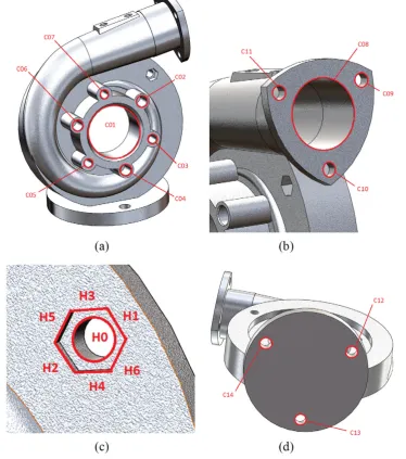
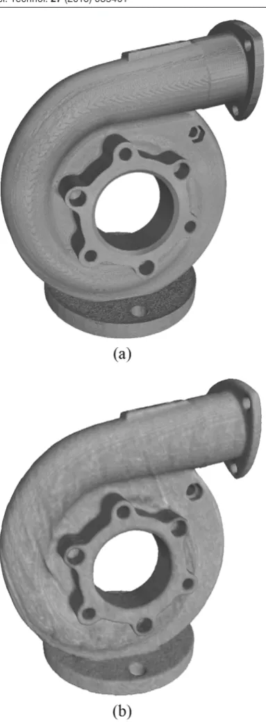
An exemplar component was designed with features represen-tative of a typical request for measurement by industry. A turbo-charger design was selected as shown in figure 1 with features large enough to be identified within the RTT baggage scanner, but the entire housing kept small enough such that it would fit within the field of view of the lab-based CT scanner (and hence the RTT baggage scanner). The component was 3D printed in ABS plastic on the ‘Fortus 400MC FDM’ (Stratasys, USA) which has a resolution of approximately 0.05 mm. Plastic was chosen for ease of penetration in the x-ray CT scanners while

this particular component would typically be manufactured from steel; the power of the current RTT baggage scanner is suited to polymers and light alloy components.

The final CAD model defined a 260 mm  ×260 mm  × 150 mm  volume containing a 60 mm central bore (labelled C01) surrounded by a number of holes for ranging from 9 mm to 12 mm (labelled C02–C07), a hexagonal seating (labelled H) for one hole (labelled H0), and a 45 mm inlet (labelled C08) with a tapering diameter spiralling to the centre sur-rounded by three 9 mm fixture holes (labelled C09–C11).

Further the design incorporated a flat base with the housing mounted at an angle to reduce potential CT related artefacts on the housing itself that could arise where items are parallel to the beam path. The base contains three cylindrical holes (labelled C12–C14) used for mounting and which would fur-ther be used to provide measurements for voxel scaling within CT scans as discussed in section 3.3.

2.2. CMM confirmation

Dimensional information on the features to be evaluated were obtained using a ‘LK HG90 CMM’ (Nikon metrology, UK) with touch probes in a temperature controlled environ-ment, at a standard 20 °C for the duration of measurement. The repeatability is 6 μm and the manufacturers specifica-tion of the machine when verified to ISO 10360-2 [3] was determined with a test uncertainty of (  _{1.0 m}µ +_{1.0 m m} µ   −1) (k = 2) according to ISO 23165 [41]. This level of accuracy is suitable to assess the CT measurements given the voxel sizes are orders of magnitude larger; approximately 0.138 mm and 1.180 mm in the Nikon and Rapiscan systems respectively.

To transfer the global coordinate frame of the CMM into the local part coordinate frame of the ALM printed comp-onent several datums are required. A plane was constructed across the central bore that contains holes C02–C07, and a line between the centres of holes C02 and C06 as identifiable in figure 1. To perform the alignment procedure, the plane was used as the primary axis, the constructed line between C02 and C06 was used as the secondary axis and the centre of hole C06 was used as the tertiary axis. Following the alignment process, measurement of individual features were performed.

2.3. Lab-based x-ray CT

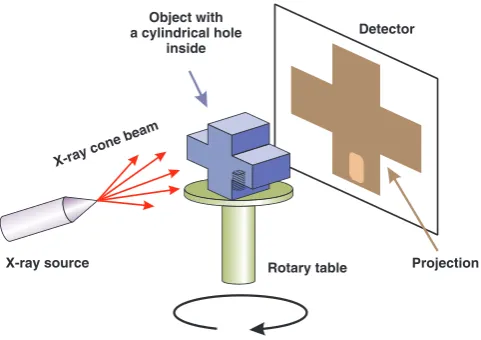
The typical setup for lab-based cone-beam x-ray CT is shown in figure 2 comprising of an x-ray source with a spot size to the order of micrometres, a receiving area detector with the sample placed on a manipulator in the path of the x-ray beam.

As x-rays interact with the object they are attenuated due to absorption or scattering. X-rays that continue to traverse the sample are received by the area detector. The proportion of x-ray energy received when an object is in the beam path is compared to the relative energy received when it is not results in a 2D grey scale image of the object, where the grey value is dependent on the amount and type of material the x-rays have interacted with. The object is rotated in the x-ray beam path with radiographs taken at angular increments through 360 degrees. These radiographs are then reconstructed to gen-erate a 3D model normally through a method of filtered back projection [42, 43].

The lab-based CT scanner used in this study was the ‘Nikon XT H 225/320 LC’ (Nikon Metrology, UK) with the scanning parameters shown in table 1 resulting in a total acquisition time of 1570 s. The detector consists of 200 μm pixels arranged in a 2000×2000 array. A higher resolution could be achieved through detector mosaics or stitching several scans together but this could introduce further error, and for these reasons the collection of images was completed in a single scan. This scan provided a benchmark to compare against the lower resolution scans achieved from the RTT baggage scanner.

2.4. Real Time Tomography (RTT)

The system used in this study was the ‘Rapiscan RTT110’

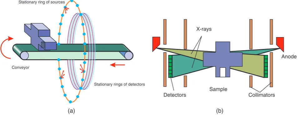
(Rapiscan Systems, UK) shown in figure 3, similar to that described in US patents [37, 38]. The RTT airport baggage scanner operates very differently to lab-based CT and is more akin to medical devices in its arrangement. As shown in figure 4(a) the setup consists of stationary rings of sources and detectors around the object that fire in a designated order to acquire radiographs at a number of angles while the object tra-verses the conveyor belt. This type of acquisition is essentially a multiple fan-beam setup given the small detectors and trans-lations of the object relative to the source/detector geometry as in figure 4(b). A comparison between laboratory, medical and RTT imaging methods is shown in figure 5.

It consists of approximately 900 sources operating at 160 kV voltage, 20 mA current with exposure times to the order of 100 μs, observed by a multi ring detector array.

Figure 2. A typical lab-based cone beam x-ray CT setup consisting of a source and detector with a rotary sample stage for the object. Images are collected through a full 360 degrees rotation of the object that are then reconstructed to a 3D model.

X-ray con e beam

X-ray source _{Rotary table}

Detector

Projection Object with

a cylindrical hole inside

Table 1. Nikon scanning parameters.

Parameter Value

Voltage (kV) 120

Current (μA) 90

Exposure (ms) 500

Projections 3142

Voxel size (μm) 137

Each detector is a multi-row scintillation detector consisting of a photodiode array. The rings of sources and detectors are held stationary in a gantry, where individual sources are switched at 15 source revolutions per second to obtain part of the projection image [38, 49]. The concatenation of spe-cific projections result in a radiograph as traditionally seen in lab-based CT, and radiographs are generated for a number of angular projections. The conveyor belt is 5 m in length and has been adapted to run at speeds of 250–500 mm s−1 _through the centre of the source/detector ring allowing magnification such that the voxel size is approximately 1 mm. For the man-ufactured component that is 270 mm in length with the belt running at the slower speed of 250 mm s−1 _{the scan duration} was just 1.08 s, more than 1450 times faster than the lab-CT system. The tunnel of the Rapiscan RTT110 has a D-shape with a maximum height of 0.75 m, allowing a sample of maximum diameter 0.6 m and length of 1.0 m to be scanned. This is significantly larger than the Nikon machine used in this study which can image a 280 mm diameter object at its lowest magnification.

The unique setup requires a modified filtered back-projec-tion reconstrucback-projec-tion algorithm from that typically used as spec-ified in US patent 8135110 B2 [44]. Slices are reconstructed while the part is being scanned and is performed on multiple GPU’s producing 240 reconstructed slices a second. Given that their system is not typically used for measurement work but just inspection, the voxel size must be scaled as discussed in section 3.3.

2.5. Measurement strategy

Features identified in figure 1 were measured on the CMM to provide an accurate dimension against the CAD model. For the purpose of this study the diameter of the holes were considered for C01–C11 and the centre to centre distances of holes C12–C14 as given in section 3.1.

Three CT scans were performed using the Rapiscan system each taking approximately one second to complete. The

component was placed flat on the conveyor belt in different orientations, with vertical orientations precluded as the lead curtains of the system often interfered causing the object to fall or wobble during the scan. The reconstruction to a 3D model requires no user intervention and takes less than a second. The results were then imported into ‘VG Studio Max’ (Volume Graphics, Germany) for dimensional evaluation. This process can be automated by the use of macros within the software and its speed is scalable dependent on system hardware, so in theory could again provide measurements in a fraction of a second.

From the CT scans the centre to centre distances of holes C12–C14 were measured. Given these values and that obtained by the CMM a voxel scaling can be calculated by method of least squares as discussed by Lifton et al [34]. While this is good practice for all CT measurement work, it was part-icularly important in this instance given that the scanner is not a dimensionally calibrated piece of equipment and its standard applied voxel size could be (significantly) incorrect. With a satisfactory scaling in place the diameter of holes C01–C11 and the distance between opposite sides of hexagon H were measured. These dimensions were then evaluated against the calibrated CMM measurement to gain an understanding of the accuracy of the system.

For comparison the same procedure was followed for the lab-based CT system to demonstrate what is currently achiev-able in a typical CT system (without any stitching between scans). The advantage of using x-ray CT is that internal measurements can be taken, inaccessible by CMM. Circular diameters of the internal tapered cylinder were evaluated and compared to the CAD model. Due to the resolution of the ALM printing process there is expected to be some form error, and so this is evaluated by proximity to dimensional results from the Nikon scan. Further a nominal/actual com-parison with the CAD model is performed for the entire part to produce a distribution of form variations. Again, due to the resolution of the ALM printing process, comparison is drawn from the Rapiscan result to the Nikon result.

Figure 4. (a) The object enters the field of view on a conveyor belt through the centre of a ring of sources and detectors. (b) Cross sectional view of the source/detector geometry.

Stationary ring of sources

Stationary rings of detectors Conveyor

Collimators

Anode

Sample Detectors

(a) (b)

3. Results

3.1. CMM measurements

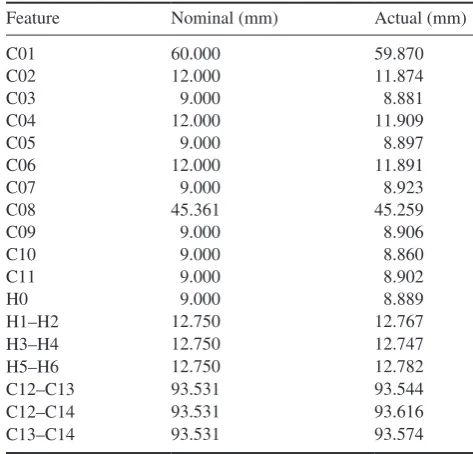
The verified CMM was used to find the dimensions of the features of the manufactured component as discussed in section 2.1. The diameter of the holes and the centre-to-centre distances against nominal measurements from the CAD model are shown in table 2. Due to the ALM layering method, there is a measurable variation from the nominal at the resolution of the CT scanner, and hence the CMM measurements are used as a point of comparison.

3.2. X-ray CT volumes

The manufactured component was scanned three times in dif-ferent orientations in the Rapiscan machine and once in the Nikon scanner as discussed in section 2.3. The resultant vol-umes were loaded into VG Studio Max as seen in figure 6 for a visual inspection and evaluation of scan quality. A 3D visuali-sation was generated by selection of an appropriate grey level threshold according to the separation of peaks as described by Otsu [45]. This threshold will continue to be used throughout the rest of the analysis.

Figure 5. Comparison of hardware arrangements of laboratory CT, medical CT and RTT setup. Laboratory CT consists of a single active source that continuously illuminates a single detector with the object rotating during/between image acquisitions taken at time Ti. In medical

CT the object remains stationary while the single source and detector rotate in a gantry around the object. RTT consists of multiple sources that fire one at a time to illuminate a group of detectors within the array held stationary in the gantry.

Laboratory CT RTT

Active sources

Inactive sources Time = T1

Time = T0

Time = T2

Medical CT

The impact of resolution is evident in these visualisations where the Nikon scan is significantly better defined than the Rapiscan example. It is notable that there is some banding in the Rapiscan volume which is an imaging artefact likely resulting from the default combination of frame rate of the detectors and belt speed. A slow frame-rate comparable to the belt speed would result in a gap in the data so it is assumed that the default reconstruction interpolates data using a simple approach. At this stage of evaluation the reconstruction prop-erties are an unknown quantity contributing to tomographic artefacts and hence measurement uncertainty, but in principal reducing the belt speed would reduce this effect. The upper and lower surfaces of the base on the Nikon volume has been subject to noise, an artefact of being near parallel to the beam path that is known to occur [14]. This has not impacted the measurement results of the holes in the base that were subse-quently used for voxel scaling. It is known that the cone beam geometry creates its own imaging artefacts, largely position related, such that the further you are from the central slice the worse the artefacts produced [22] although they are not quali-tatively obvious in the current reconstruction.

3.3. Voxel scaling

The magnification of an object within the CT scanner defined as the ratio of the source–detector distance and source–object distance along with the detector pixel size determines the equivalent pixel size within a single image. In lab-based cone beam CT the reconstruction is then assumed to have a voxel size with lengths equal to this pixel size. This can be affected by a number of variables to include sample stage position calibration, variability in the source and detector alignments, off-axis rotation and reconstruction quality to name a few.

Measurement studies on calibrated CT machines found in lit-erature report typical variations in voxel size to be approxi-mately ±1%, but given the aforementioned variability that differs from one machine to the next and further in sequential scans on a particular machine, voxel scaling should be applied on a case by case basis to ensure precision. In the case of the modified RTT scanner, no calibration has been performed making this process essential for any measurement work. For this reason a method to scale the voxels for a particular scan is required.

To do so a common method is to use ‘threshold inde-pendent’ measurements; that is dimensions that are inde-pendent of threshold selection for the object material [33, 34]. Typically this would be one or more centre-to-centre distances of features where the dimensions are known. With one centre-to-centre distance known, a single scaling can be applied to the x–y–z size of the voxel. With three centre-to-centre dis-tances and positions of the centres known it is possible using simple geometry to scale each dimension of the voxel sepa-rately. This is performed by solving the system of equations

= − − − − − − − − − − − − ⎡ ⎣ ⎢ ⎢ ⎢ ⎢ ⎤ ⎦ ⎥ ⎥ ⎥ ⎥ ⎡ ⎣ ⎢ ⎢ ⎢ ⎢ ⎤ ⎦ ⎥ ⎥ ⎥ ⎥ ⎡ ⎣ ⎢ ⎢ ⎢ ⎤ ⎦ ⎥ ⎥ ⎥

x y z

x y z

x y z

v v v d d d x y z C12 C13 2 C12 C13 2 C12 C13 2 C12 C14 2 C12 C14 2 C12 C14 2 C13 C14 2 C13 C14 2 C13 C14 2 2 2 2 C12 C13 2 C12 C14 2 C13 C14 2 (1)

where xC12 C13− is the x distance between C12 and C13 in voxels (similar for y and z and other distance features), vx, vy,

vz is the voxel side length for x, y and z, and dC12 C13− is the actual distance between C12 and C13 in mm. This system will not have an exact solution so the best fit solution for vx, vy,

vz must be calculated that minimises the error in determining

−

dC12 C13, dC12 C14− , dC13 C14− . This can be done by a simple least squares method.

Each volume was loaded into ‘VG Studio Max’ to cal-culate values required to determine the voxel scaling. First the threshold was selected as discussed in the previous sec-tion  providing an iso-surface from which all measurements would be taken. Each hole C12–C14 was fitted with a cylinder using a Gaussian least squares fitting method against approxi-mately 100 user defined points, with the cylinder extending from the top to bottom of the base plate. The centres of these cylinders were used to define centre to centre distances of the holes based on voxel coordinates, providing data required to apply the scaling.

The scaling was calculated for each scan as shown in table 3 individually as opposed to applying an average scaling across the repeated scans from the Rapiscan. The voxel size that was previously unknown for the Rapiscan scanner aver-ages 1.1840 mm  ×1.1848 mm  ×1.0430 mm  . The scaled voxel size for the Nikon scanner was essentially cubic, as one would expect, with variations to the order of 0.0002 mm. It could be argued that the fit for the Nikon system should remain cubic and to reduce the degrees of freedom, but items such as detector warp could cause non-cubic results. The resultant nominal/actual differences for the centre-to-centre distances against that measured by the CMM were larger in the first Rapiscan evaluation, but interestingly the scalings appear to

Table 2. CMM measurements (actual) of manufactured component features compared to nominal values defined in the CAD model (nominal).

Feature Nominal (mm) Actual (mm)

C01 60.000 59.870

C02 12.000 11.874

C03 9.000 8.881

C04 12.000 11.909

C05 9.000 8.897

C06 12.000 11.891

C07 9.000 8.923

C08 45.361 45.259

C09 9.000 8.906

C10 9.000 8.860

C11 9.000 8.902

H0 9.000 8.889

H1_–H2 12.750 12.767

H3_–H4 12.750 12.747

H5_–H6 12.750 12.782

C12–C13 93.531 93.544

C12–C14 93.531 93.616

C13–C14 93.531 93.574

be closest to the nominal overall in the second Rapiscan evalu-ation although the Nikon scanner provides an extremely accu-rate measurement of C12_–C13 with zero variation at the order of magnitude of the results.

3.4. Dimensional measurements

With the scaling applied dimensional measurements of the previously described features were taken. A cylinder was fitted to each hole using the same Gaussian best fit method as in the voxel scaling and the diameter recorded. In the case of the hexagon a plane was defined on each side from which the

perpendicular distance to the opposite plane was determined. These measurements were then compared to the CMM result to evaluate the accuracy of the system.

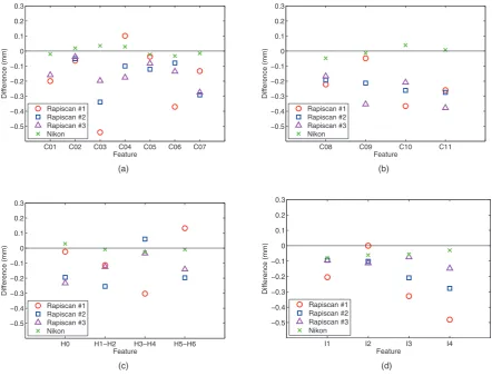
First consider variation in measured hole diameters C01–C07 shown in figure 7(a) that are located around the central region of the manufactued component shown in figure 1. It is noteworthy that all measurements in this section are sub-voxel in accuracy. This is to be expected and has been shown by a number of previous authors [9, 27, 30–32] that the method of voxel scaling can frequently result in such an occurrence. The Nikon measurements are naturally the most accurate given the resultant voxel size is nearly 7.5 times smaller, but this does not necessarily equate to a proportional increase in measurement accuracy due to other source of error that can occur within x-ray CT. The majority of measurements from the Rapiscan evaluation are negative, i.e. smaller than measured by the CMM (with the exception of one), which has been shown to occur in some inner dimension measurements [24]. The larger 12 mm surrounding holes C02, C04, C06 averaged an error in magni-tude of −0.101 mm for the Rapiscan compared to an average absolute error of 0.027 mm for the Nikon scan. Similar con-sideration given to the smaller 9 mm holes results in average absolute errors 0.224 mm and 0.024 mm for the Rapiscan and Nikon respectively. The variation in the Rapiscan evaluation is more than twice than experienced for the 12 mm holes which is to be expected given that the holes are represented by pro-portionally fewer voxels. It is the 9 mm hole C03 measured in the first Rapiscan evaluation that gives the largest error of the entire measurement study equal to −0.541 mm, still approxi-mately half the voxel size. The number of voxels representing a hole is limiting in increasing accuracy by the voxel size itself as can be seen by comparing these errors to the larger central bore which has a diameter of 60 mm; the average absolute error in the Rapiscan evaluation is still 0.148 mm.

Next consider the variation in measured hole diameters C08–C11 located at the inlet as shown in figure 7(b). Similar observations can be made regarding the comparison of meas-urement accuracy capability of the Rapiscan and Nikon scans given the available voxel size. Holes C09–C11 lie on a plate around the inlet that is 10 mm thick. Measurement of hole C09 in the first Rapiscan run is particularly close to the CMM meas-urement with a difference of 0.040 mm, a resolution equivalent to 0.05 voxels, but if the achieved values were considered in their own right against the other Rapiscan measurements this might have infact been considered an anomaly in a measure-ment study. These holes had an average measuremeasure-ment error of 0.263 mm and 0.020 mm for the Rapiscan and Nikon scans respectively, comparable to the accuracy achieved for the same size 9 mm holes measured around the bore. The inlet hole C08 showed a measurement accuracy comparable to the bore C01.

Finally the variation in the hexagonal seating H1–H6 and internal hole H0 is given in figure 7(c). The hexagon had sides of length 7.36 mm at a depth of 4 mm so a particularly accurate measurement using the Rapiscan volumes was not expected given its representation by so few voxels. Despite this the difference compared to the CMM measurement was still comparable to features C01–C11. The distance between sides of the hexagons predominantly shows under-estimates

in the Rapiscan evaluation but two are over-estimates, with a mean absolute error of 0.151 mm which is surprisingly better than the 9 mm hole measurement accuracy. The hole H0 showed under-estimates against the CMM measurement, the same as all other holes (except C04).

3.5. Internal dimensions

One of the advantages of CT is that internal measurements can be taken non-destructively that cannot be reached by traditional

metrological methods such as tactile CMM. Internal form can affect part performance and can be of significant interest to manufacturers; for example in the case of a turbo charge it could affect the airflow. The manufactured component con-sists of a tapered cylinder that rotates around the central bore providing a point of measurement. Comparisons given here are against the CAD model as no CMM measurements are available, hence there is expected to be a slightly larger error than previous measurements given the deviation from the nominal that has been able to be measured shown in table 2.

Table 3. Voxel scaling results for each of the three Rapiscan and single Nikon CT scans.

CMM (mm) Rapiscan #1 (mm) Rapiscan #2 (mm) Rapiscan #3 (mm) Nikon (mm)

Voxel scaling

x 1.176 44 1.187 05 1.188 63 0.137 89

y 1.183 99 1.185 97 1.184 40 0.137 87

z 1.047 90 1.039 05 1.041 97 0.137 69

Centre-to-centre distances

C12–C13 93.544 93.403 93.556 93.577 93.544

C12–C14 93.616 93.678 93.592 93.528 93.578

C13–C14 93.575 93.654 93.586 93.629 93.612

Nominal/actual difference

C12_–C13 −0.141 0.012 0.033 0.000

C12_–C14 0.062 −0.024 −0.088 −0.038

C13–C14 0.080 0.012 0.055 0.038

Note: Shown is the calculated scaled voxel size, the resultant centre to centre distances and how this compares with the value measured by the CMM.

Figure 7. (a)–(c) Differences of the CT scan measurement to the CMM measurement for all features given in table 2. (d) Difference of the internal circle measurements prescribed in figure 8 against the CAD measurement.

C01 C02 C03 C04 C05 C06 C07 −0.5

−0.4 −0.3 −0.2 −0.1 0 0.1 0.2 0.3

Difference (mm)

Feature Rapiscan #1

Rapiscan #2 Rapiscan #3 Nikon

(a)

C08 C09 C10 C11 −0.5

−0.4 −0.3 −0.2 −0.1 0 0.1 0.2 0.3

Difference (mm)

Feature Rapiscan #1

Rapiscan #2 Rapiscan #3 Nikon

(b)

H0 H1−H2 H3−H4 H5−H6 −0.5

−0.4 −0.3 −0.2 −0.1 0 0.1 0.2 0.3

Difference (mm)

Feature Rapiscan #1

Rapiscan #2 Rapiscan #3 Nikon

(c)

I1 I2 I3 I4 −0.5

−0.4 −0.3 −0.2 −0.1 0 0.1 0.2 0.3

Feature

Difference (mm)

Rapiscan #1 Rapiscan #2 Rapiscan #3 Nikon

The CAD model was imported into the evaluation software and the scan volumes aligned against the CAD using the same datums as in the CMM confirmation discussed in section 2.2. With alignment complete, four circles I1–I4 were defined in the same plane of both volumes for evaluation as shown in figure 8. The circles were defined in the plane perpendicular to the direction of curvature of the tapered cylinder with results shown in figure 7(d).

Circles I1–I4 had dimensions 39.014 mm, 29.909 mm, 20.904 mm and 13.462 mm respectively measured from the CAD model. All the Nikon measurements were smaller than the CAD dimensions, but this was to be expected given that the CMM measurements showed that all diameter features devi-ated from the CAD in a negative way as observed in table 2

and is a result of the manufacturing process. Measurement of all external features C01–C11 and hexagon H in the Nikon scan were within ±0.035 mm of the achieved CMM values, so one could reasonably assume the actual dimensions of circles I1–I4 are within similar bounds. Even with the precise meas-urement of the circles unknown, it is clear that once again all measurements are sub-voxel in accuracy. Circle I4 produces the largest differences, attributed to its comparatively smaller size and being surround by significantly more material than I1 and I4.

3.6. Actual/nominal comparison

Inherently every manufacturing process imparts variations from sample to sample which can have implications where the part has features that have specific conformance metrics in order to achieve the correct functional fit. In the example of this turbo-charger the position of the inlet flange C08 needs to be accurately controlled relative to the central bolting region such that with part fixed in place, the inlet flange connects

comfortably to piping that feeds from the exhaust. To evaluate such deviations from functional tolerances it is typical to per-form a nominal/actual comparison relative to set datums. This component has been manufactured through ALM, so while individual features such as holes will have relatively small dimensional deviations against the CAD as shown in table 2

the distance between them will be subject to greater devia-tions through the lay-up process.

CT has significant time advantages over tactile CMM to evaluate deviations over the surface. Although the data col-lected from a tactile CMM would be orders of magnitude more accurate, it would be impractical to obtain the same quantity of data. Even at the resolution of the Rapiscan volume there are in excess of 75 000 external surface voxels. Given that it takes discrete point tactile CMM 1 s to measure one point in addition to the time to move the probe into place, it is entirely unfeasible to obtain the same spatial distribution of devia-tions. In addition, internal features are largely impossible to measure using CMM as these items would typically be inac-cesible. In a single scan, CT can obtain the data for quantifi-cation of all internal and external features much faster than what is currently possible with tactile CMM. At the expense of accuracy this data can be achieved faster than typical lab-based CT with the proposed Rapiscan machine.

A resolution performance evaluation can be extracted by performing a nominal/actual comparison of the Rapiscan vol-umes against the Nikon volume by aligning through a best fit procedure that minimises the distance between the two sur-faces. This alignment will identify how the lower resolution has affected the measurement of individual features. A visual representation of the comparison is shown in figure 9. On a local scale individual banding in the Rapiscan volumes that is an artefact of orientation are evident, while globally the varia-tions are largely the same.

Even with the banding artefact discussed in section 3.2

the surface variation compared to the Nikon shows largely the same deviations between each Rapiscan volume, i.e. the global variation is orientation independent. Externally there are two regions with large negative deviations on the periphery of the tapered cylinder observable in the top left and bottom right region of figure 9(a). The circular feature con-taining holes C01–C08 also shows areas of negative deviation while the holes themselves show a relatively even distribution of deviations about zero. The internal tapering cylinder has one side where the deviations are positive and one side where the deviations are negative implying that there is a positional bias resulting from the lower resolution. The base plate shows strong positive variance, but an error here was expected as the Nikon scan displayed noise in this region as discussed in section 3.2. In subsequent numerical analysis the base plate was ignored as the deviation was largely due to artefacts as opposed to being a true representation of that region.

A statistical evaluation of the surface deviations against the Nikon volume is given table 4. The distribution of deviations is normal, centred relatively close to zero although slightly negative as expected from the form evaluation in figure 10. It is interesting to consider the value of one standard deviation as in the context of the normal distribution the data within

one standard deviation represents 65% of the values. That is 65% of the deviations are within approximately 0.25 mm of the Nikon volume. Further 95% of values are within approxi-mately 0.60 mm of the Nikon volume. The difference is again sub-voxel but not to the magnitude of the feature measure-ments presented earlier in the study. This is because individual feature measurements average surface point measurements

that are each subject to deviations, and so a smaller error results.

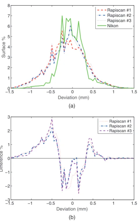
With an understanding of the impact of resolution on the evaluation of surface devations, a nominal/actual comparison was performed for the CAD against the achieved CT volumes. This process evaluates the functional fit of component given build errors inherent in the manufacturing process; in this case ALM. The CT volumes were aligned against the CAD as per-formed during CMM measurement; a plane was constructed across the central bore that contains holes C02–C07, and a line was constructed between the centres of holes C02 and C06 were measured as identifiable in figure 1. In this align-ment procedure it reasons that surface points further from the initial datums will demonstrate greater deviations as a result of the ALM lay-up process.

A histogram of surface deviations of each CT volume is shown in figure 10(a). The results from the higher resolu-tion Nikon scan show a gaussian distriburesolu-tion of the deviaresolu-tions with the 82% of points within ±0.5 mm. With this information a manufacturer can decide if the component build is within

Figure 9. Actual/nominal comparison of Rapiscan volume (#1) to Nikon volume. (a) 3D view of external deviations. (b) Clipped 3D view to show internal deviations. The scale has been clipped at ±0.5 mm (beyond which there is no change in colour) to emphasize differences between volumes.

Table 4. Statistical data from actual/nominal comparison of volumes between Rapiscan volumes and Nikon volume showing the minimum, maximum and mean deviations, the standard deviation and the error at the 95th percentile.

Rapiscan #1 Rapiscan #2 Rapiscan #3

Min. (mm) −1.425 −1.419 −1.421

Max. (mm) 1.050 1.038 1.041

Mean (mm) −0.075 −0.063 −0.067

Std. dev. (mm) 0.230 0.248 0.246

95th % (mm) 0.599 0.525 0.549

Figure 10. Actual/nominal comparison of CT volumes to CAD model using the same alignment strategy as the CMM measurements. (a) Deviations from the surface as a percentage of the surface. (b) Difference between deviations for the Nikon volume against the Rapiscan volumes.

−1.50 −1 −0.5 0 0.5 1 1.5 1

2 3 4 5 6 7 8

Deviation (mm)

Surface

%

Rapiscan #1 Rapiscan #2 Rapiscan #3 Nikon

(a)

−1.5 −1 −0.5 0 0.5 1 1.5

−3 −2 −1 0 1 2 3

Deviation (mm)

Difference

%

Rapiscan #1 Rapiscan #2 Rapiscan #3

tolerance for the functional fit, and if not modify their build process accordingly. Having been performed with lab-based CT the scan times are too long to incorporate such a comparison in a production line environment, so it is of interest to see compare performance with the Rapiscan volumes assuming the Nikon results to be the benchmark. In figure 10(a) while the Rapiscan histograms similarly show a gaussian distribution the spread is much wider such that only approximately 58% of points are within ±0.5 mm. The greater deviations exist in the regions shown to have large variations from the Nikon volume observed in figure 9, with the negative skew arising from the prominent negative region at the top of the curve of inlet near the flange.

The variation in the nominal/actual comparisons are fur-ther highlighted in figure 10(b) where the difference between the CAD/Nikon and CAD/Rapiscan deviations is shown. Encouragingly, the histograms in figure 10(b) are broadly the same, indicating there is only a local dependence on object orientation throughout scanning. This much more clearly highlights the negative skew observed in figure 10(a) shown by the larger peak for negative deviation. The tendency to under-estimate rather than over-estimate in Rapiscan results seems to be a common theme with direct feature measure-ments in section 3.4 showing the same characteristic.

4. Discussion

Unsuprisingly, the measurement of the features were signifi-cantly closer to the values achieved by the CMM in the Nikon CT scan than the Rapiscan due to the greater resolution and better signal to noise in the radiographs. Further there is a greater consistency in Nikon measurements in that they are equally distributed around the CMM measurements. In fact the Nikon measurements compared to the CMM are within the 0.04 mm resolution of the ALM printer. By contrast, the Rapiscan results frequently under-estimated the size of the features which implies there is a bias. Measurement of inner diameters have previously been shown to demonstrate this bias such as in the CT Audit [24], but given that the Nikon results do not display this tendency it is proposed that this could infact be an artefact of resolution. Also it is noted that there is no information in the CT Audit if the voxels were scaled prior to measurement as performed in this study or if measurements were taken from the raw data.

The mean error in the Nikon and Rapiscan measurements were 0.024 mm and 0.176 mm respectively and the maximum error was 0.048 mm and 0.542 mm respectively. That means for a 7.5 times decrease in resolution the average error and maximum error increased by 7.3 and 11.3 times respectively. Considering the magnitude of the errors as a function of resolution all meas-urements were sub-voxel size with an average accuracy of 0.18 voxels in both the Nikon and Rapiscan measurements, and a maximum error of 0.35 voxels and 0.52 voxels in the Nikon and Rapiscan respectively. The maximal error is expected to be larger in the Rapiscan due to the smaller number of voxels representing the feature, but to obtain errors of sub-voxel magnitude for fea-tures which are less than 9 voxels in diameter is still impressive.

While the resolution of the modified baggage scanner is significantly worse than lab-CT there could be many

applications where this level of measurement is acceptable. For example there are plastics forming applications that have particularly low tolerances of approximately 0.3 mm where scans at this resolution could provide sufficient informa-tion. The vast majority of manufacturing quality applications require the resolution of lab-CT or greater, so if an increase in resolution could be achieved then this could make a signifi-cant impact. Furthermore with imaging and potential analysis speeds of one component every second, a throughput of 3600 items an hour matches many manufacturing production rates and exceeds the requirement of others.

Using CT as a quantitative assessment tool has advantages over other metrological system because it can obtain informa-tion not only on the surface, but internally. This enables both the examination of intended features for non conformance but also the absence of manufacturing defects such as pores and delamination that might arise in castings or additive manu-facture of products. With significantly shorter scan times than previously considered, the question must now be posed— ‘How long do we have to scan?’. For in-line manufacturing inspections this would largely depend on the requirement for the cycle time (number of parts assessed per hour); 3600 parts allows 1 second, 360 parts allows 10 s, 120 parts allows 30 s.

An easily applied strategy to improve the accuracy of the measurements would be to scan the part a number of times and averaging, thus increasing the scan time. If the three measure-ments per feature achieved in this study were averaged, the maximum error reduces to 0.359 mm compared to 0.542 mm when considering them individually—a 34% reduction. Further fuller statistical studies could be performed in 30 s; typically 30 measurements is required for such a study which takes consideration of normality and confidence intervals. There is a suspected bias in the results as most measurements were under-estimates which if shown to systematic, can be corrected for in an evaluation that achieves a large number of repeated measurements [46]. This then opens considerations of experimental design for statistical evaluation of which there is much applicable literature from a metrological perspective.

Voxel scaling in this study was performed by using known centre-to-centre distances on the component as is frequently perfomed in industry [33]. While this has been shown to provide measurement accuracy comparable to that of a cali-brated workpiece, current international standards require the application of such a workpiece [3, 6, 28] and has been used in standard lab CT by a number of authors [9–11, 13, 24,

26, 29, 30, 34]. The Rapiscan RTT110 machine itself was not calibrated prior to scanning like other CT scanners as its use is not intended for measurement but for threat detec-tion. This different source/detector geometry may require a slightly different workpiece to those previously described as the systematic errors will differ from coventional lab-based cone-beam CT which have yet to be fully explored. It would be the subject of a future study to garner an understanding of errors induced in this unique arrangement that would lead to the development of an appropriate workpiece to capture these effects.

a minimum size requirement for a feature to be observable at a particular voxel size. This could potentially be achieved through some operational modifications which could increase the scan time. The belt speed could be slowed from the cur-rent 250–500 mm s−1 _{such that more images can be taken as} the object traverses the conveyor belt—with more images a higher resolution reconstruction could potentially be achieved. This modification may also consider the ‘firing’ order of the sources and how this impacts the quality of the scans [47–49].

Beyond this hardware changes would have to be employed such as a smaller pixel size and denser pixel array—the caveat here is that halving the pixel size typically results in a quarter of the sensitivity and so would require a four times longer exposure. With this said, the manufactured component evalu-ated was significantly smaller than the diameter of the tunnel (0.75 m). If a machine were to be purpose built for a part-icular component (or items of this size), the ring of sources could be moved closer to the centre to increase the magnifica-tion without replacement of source or detector components, potentially resulting a voxel size of 0.35 mm given the current geometry. The alternative would be the converse where the ring of detectors could be made larger e.g. 1.5 m in diamter so more sensors could be used and increase the magnification.

Here a plastic sample was scanned due to its ease of penetra-tion and minimal beam hardening compared to metallic parts. With the current implementation the x-ray energy is set to 160 kV which is suitable for a wide range of polymers, light alloys and ceramic parts. To study large components comprising materials of high atomic mass, higher x-ray energies would be needed which poses its own set of problems with potentially larger and heavier sources that would need to be mounted on the gantry.

5. Conclusion

This study has evaluated the potential of a modified Rapiscan RTT110 airport baggage scanner as a measurement tool in the context of manufacturing quality assurance and inspection, chosen due to its exceptional scan times. While the current system is capable of spatial resolutions around 1 mm com-pared to approximately 0.137 mm of the lab CT system on the same component, it has been shown that with sub-voxel accuracy the largest error occuring in the Rapiscan system was less than 0.6 mm and an average error of approximately 0.18 mm—this was significantly better than expected.

We have demonstrated scanning a 270 mm component in 1.08 s which is more than 1450 times faster than a lab-CT system. This impressive speed-up could be reduced somewhat to improve the spatial resolution achieved for manufactured comp-onents through the suggestions made, with the onus now on industry to dictate the pace at which scanning should occur with the potential accuracy as the limiting factor. Most importantly the system is capable of examining parts at practical manufac-turing rates. Furthermore component-specific software could be developed to analysis the parts in real time with no need for accurate placement at the converyor belt. Our aim in this paper has not been to demonstrate a fully working practical solution but rather to show that new multi-source CT systems could be developed capable of in-line part inspection. This could be of

specific value for parts that may contain internal sub-surface defects such as castings and additvely manufactured parts.

In its current state the system maybe suitable for a number of sample evaluations, but some relatively simple operational changes could increase the resolution further and thus expand its application. The potential of such a system is evident and necessitates much deeper investigation that will likely result in improved resolution and accuracy, and could in the long term revolutionise in-line quality assurance in industry.

Acknowledgments

The authors would like to acknowledge the UK Research Partnership Investment Fund (UKRPIF) of the Higher Education Funding Council for England for making the RTT system available for the research presented in this study. Authors from Warwick Manufacturing Group would like to thank the HVM Catapult for their support in making this work possible and funding from EPSRC grant EP/K031066/1. Authors from the University of Manchester would like to express gratitude for funding from the Royal Society Wolfson Research Merit Award and EPSRC grant EP/M010619/1.

This article was published as open access with funding from EPSRC. All data directly related to this paper is provided in full in the results section. Please contact the corresponding author for access to additional data from this project related to the results presented above.

References

[1] JCGM 2008 International vocabulary of metrology—basic and general concepts and associated terms (VIM) JCGM 200:2008 Joint Commitee for Guides in Metrology [2] ASME 2004 Methods for performance evaluation of articulated

arm Coordinate Measuring Machines (CMM) ASME B89.4.22-2004 The American Society of Mechanical Engineers [3] ISO 10360 2011 Geometrical Product Specifications

(GPS)—Acceptance and Reverification Tests for Coordinate Measuring Machines (CMM) (International Organization for Standardization)

[4] BSI 2011 Non destructive testing—radiation methods— computed tomography BS EN 16016-3:2011 British Standards Institution

[5] ASTM 2014 Standard Guide for Computed Tomography (CT) Imaging ASTM E1441-11:2014 American Society for Testing Materials

[6] VDI/VDE 2011 Computed tomography in dimensional measurement VDI/VDE 2630 Part 1.3 Verein Deutscher Ingenieure

[7] Liu F Y N, Wu Z, Wong B T and Jeppesen R 2014

Simultaneous image distribution and archiving US Patents Specification US 8713131 B2

[8] Yancey R N, Eliasen D S, Gibson R and Dzugan R 1996 CT-assisted metrology for manufacturing applications Proc. SPIE 2948 222–31

[9] Bartscher M, Hilpert U, Goebbels J and Weidemann G 2007 Enhancement and proof of accuracy of industrial Computed Tomography CT measurements Ann. CIRP 56 495–8 [10] Carmignato S, Dreossi D, Mancini L, Marinello F, Tromba G

[11] Brunke O, Santillan J and Suppes A 2010 Precise 3D dimensional metrology using high-resolution x-ray computed tomography Proc. SPIE 7804 78040O

[12] Bartscher M, Neukamm M, Hilpert U, Neuschaefer-Rube U, Hartig F, Kniel K, Ehrig K, Staude A and Goebbels J 2010 Achieving traceability of industrial computed tomography

Key Eng. Mater. 437 79–83

[13] Kasperl S, Hiller J and Kruth J-P 2008 Computed tomography metrology in industrial research and development Int. Symp. on NDT in Aerospace (Furth, Germany) pp 139–48

[14] Kruth J P, Bartscher M, Carmignato S, Schmitt R, De Chiffre L and Weckenmann A 2011 Computed tomography for dimensional metrology CIRP Ann.—Manuf. Technol.

60 821–42

[15] Müller P, Cantatore A, Andreasen J L, Hiller J and De

Chiffre L 2013 Computed tomography as a tool for tolerance verification of industrial parts Proc. CIRP 10 125–32 [16] De Chiffre L, Carmignato S, Kruth J-P, Schmitt R and

Weckenmann A 2014 Industrial applications of computed tomography CIRP Ann.—Manuf. Technol. 63 655–77 [17] Maire E and Withers P J 2014 Quantitative x-ray tomography

Int. Mater. Rev. 59 1–43

[18] Weitkamp T and Bleuet P 2004 Automatic geometrical calibration for x-ray microtomography based on Fourier and Radon analysis Proc. SPIE Dev. X-ray Tomogr. IV

5535 623–7

[19] Welkenhuyzen F, Boeckmans B, Tan Y, Kiekens K, Dewulf W and Kruth J-P 2014 Investigation of the kinematic system of a 450 kV CT scanner and its influence on dimensional CT metrology applications 5th Conf. on Industrial Computed Tomography (ICT) (Wels, Austria) pp 217–25

[20] Hiller J, Maisl M and Reindl L M 2012 Physical

characterisation and performance evaluation of an x-ray micro-computed tomography system for dimensional metrology applications Meas. Sci. Technol. 23 085404 [21] Vogeler F, Verheecke W, Voet A, Kruth J-P and Dewulf W

2011 Positional stability of 2D x-ray images for computer tomography Int. Symp. on Digital Industrial Radiology and Computed Tomography (Berlin, Germany)

[22] Kumar J, Attridge A, Wood P K C and Williams M A 2011 Analysis of the effect of cone-beam geometry and test object configuration on the measurement accuracy of a computed tomography scanner used for dimensional measurement Meas. Sci. Tehnol. 22 035105

[23] Weiß D, Lonardoni R, Deffner A and Kuhn C 2012 Geometric image distortion in flat-panel x-ray detectors and its influence on the accuracy of CT-based dimensional measurements 4th Conf. on Industrial Computed

Tomography (ICT) (Wels, Austria) pp 175–81

[24] Carmignato S 2012 Accuracy of industrial computed tomography measurements: experimental results from an international comparison CIRP Ann.—Manuf. Technol. 61 491–4 [25] Dewulf W, Tan Y and Kiekens K 2012 Sense and non-sense

of beam hardening correction in CT metrology CIRP Ann. Manuf. Technol. 61 495–8

[26] Bartscher M, Sato O Härtig F and Neuschaefer-Rube U 2014 Current state of standardization in the field of dimensional computed tomography Meas. Sci. Techol.

25 064013

[27] ISO 15530 2011 Geometrical Product Specifications (GPS)—

Coordinate Measuring Machines (CMM): Technique for Determining the Uncertainty of Measurement (International Organization for Standardization)

[28] Weckenmann A and Kramer P 2009 Assessment of measurement uncertainty caused in the preparation of measurements using computed tomography XIX IMEKO World Congress, Fundamental and Applied Metrology

(Lisbon, Portugal) pp 1888–92

[29] Jimenez R, Ontiveros S, Carmignation S and Yague J A 2012 Correction strategies for the use of a conventional micro-CT

cone beam machine for metrology applications Proc. CIRP

2 34–7

[30] Müller P, Hiller J, Cantatore A and De Chiffre L 2012 A study on evaluation strategies in dimensional x-ray computed tomoraphy by estimation of measurement uncertainities Int. J. Metrol. Qual. Eng. 3 107–15

[31] Müller P, Hiller J, Dai Y, Andreasen J L, Hansen H N and De Chiffre L 2014 Estimation of measurement uncertainties in x-ray computed tomography metrology using the substitution method CIRP Ann.—Manuf. Technol.7 222–32 [32] Leonard F, Brown S B, Withers P J, Mummery P M and

McCarthy M B 2014 A new method of performancy verification for x-ray computed tomography measurements

Meas. Sci. Technol. 25 065401

[33] Kiekens K, Welkenhuyzen F, Tan Y, Bleys P H, Voet A, Kruth J-P and Dewulf W 2011 A test object with parallel grooves for calibration and accuracy assessment of industrial computed tomography CT metrology Meas. Sci. Technol. 22 115502

[34] Lifton J J, Malcolm A A, McBride J W and Cross K J 2013 The application of voxel size correction in x-ray computed tomography for dimensional metrology Int. NDT Conf. and Exhibition (Singapore) pp 19–20

[35] Brunke O, Lübbehüsen J, Hansen F and Butz F F 2013 A New Concept for High-Speed Atline and Inline CT for up to 100% Mass Production Process Control 16th Int. Congress of Metrology P06003

[36] Singh S and Singh M 2003 Explosives detection systems (EDS) for aviation security Signal Process. 83 31–55 [37] Morton E J 2010 X-ray monitoring US Patent US 7724868 B2 [38] Morton E J 2015 X-ray scanners US Patent US 9020095 B2 [39] Flitton G, Breckon T P and Megherbi N 2013 A comparison

of 3D interest point descriptors with application to airport baggage object detection in complex CT imagery Pattern Recognit. 46 2420–36

[40] Thompson W M, Lionheart W R B, Morton E J,

Cunnigham M and Luggar R D 2015 High speed imaging of dynamic processes with a switched source x-ray CT system Meas. Sci. Technol. 26 055401

[41] ISO 23165 2006 Geometrical Product Specifications (GPS)—Guidelines for the Evaluation of Coordinate Measuring Machine (CMM) Test Uncertainty (International Organization for Standardization)

[42] Natterer F and Wübbeling F 2001 Mathematical methods in image reconstruction (SIAM: Mathematical modeling and computation) (Philadelphia: Society for Industrial and Applied Mathematics)

[43] Kak A C and Slaney M 2001 Principles of computerized tomographic imaging (SIAM: Classics in applied mathematics) (Philadelphia: Society for Industrial and Applied Mathematics)

[44] Morton E J 2012 X-ray tomography inspection systems US Patent US 8,135,110 B2

[45] Otsu N 1975 A threshold selection method from gray-level histograms Automatica11 23–7

[46] O’Donnell G E and Hibbert D B 2005 Treatment of bias in estimating measurement uncertainty Analyst 130 721–9 [47] Thompson W M, Lionheart W R B and Öberg D 2013

Reduction of periodic artefacts for a switched-source x-ray CT machine by optimising the source firing pattern

The 12th Int. Meeting on Fully Three-Dimensional Image Reconstruction in Radiology and Nuclear Medicine

(Newport, USA) pp 345–8

[48] Betcke M M and Lionheart W R B 2013 Multi-sheet surface rebinning methods for reconstruction from asymmetrically truncated cone beam projections: I. Approximation and optimality Meas. Sci. Technol.26 055401