warwick.ac.uk/lib-publications
Original citation:
Marcin, Jurdzinski and Lazic, Ranko (2017) Succinct progress measures for solving parity
games. In: 32nd Annual ACM/IEEE Symposium on Logic in Computer Science (LICS),
Reykjavik, Iceland, 20-23 Jun 2017. Published in: Proceedings of the 32nd Annual ACM/IEEE
Symposium on Logic in Computer Science (LICS).
Permanent WRAP URL:
http://wrap.warwick.ac.uk/87818
Copyright and reuse:
The Warwick Research Archive Portal (WRAP) makes this work by researchers of the
University of Warwick available open access under the following conditions. Copyright ©
and all moral rights to the version of the paper presented here belong to the individual
author(s) and/or other copyright owners. To the extent reasonable and practicable the
material made available in WRAP has been checked for eligibility before being made
available.
Copies of full items can be used for personal research or study, educational, or not-for profit
purposes without prior permission or charge. Provided that the authors, title and full
bibliographic details are credited, a hyperlink and/or URL is given for the original metadata
page and the content is not changed in any way.
Publisher’s statement:
“© 2017 IEEE. Personal use of this material is permitted. Permission from IEEE must be
obtained for all other uses, in any current or future media, including reprinting
/republishing this material for advertising or promotional purposes, creating new collective
works, for resale or redistribution to servers or lists, or reuse of any copyrighted component
of this work in other works.”
A note on versions:
The version presented here may differ from the published version or, version of record, if
you wish to cite this item you are advised to consult the publisher’s version. Please see the
‘permanent WRAP URL’ above for details on accessing the published version and note that
access may require a subscription.
Succinct progress measures for solving parity games
Marcin Jurdzi´nski and Ranko Lazi´c
DIMAP, Department of Computer Science, University of Warwick, UK
Abstract—The recent breakthrough paper by Calude et al. has given the first algorithm for solving parity games in quasi-polynomial time, where previously the best algorithms were mildly subexponential. We devise an alternative quasi-polynomial time algorithm based on progress measures, which allows us to reduce the space required from quasi-polynomial to nearly linear. Our key technical tools are a novel concept of ordered tree coding, and a succinct tree coding result that we prove using bounded adaptive multi-counters, both of which are interesting in their own right.
I. INTRODUCTION
A. Parity games
Aparity game is a deceptively simple combinatorial game played by two players—Even and Odd—on a directed graph. From the starting vertex, the players keep moving a token along edges of the graph until a lasso-shaped path is formed, that is the first time the token revisits some vertex, thus forming a loop. The set of vertices is partitioned into those owned by Even and those owned by Odd, and the token is always moved by the owner of the vertex it is on. Every vertex is labelled by a positive integer, typically called itspriority. What are the two players trying to achieve? This is the crux of the definition: they compete for the highest priority that occurs on the loop of the lasso; if it is even then Even wins, and if it is odd then Odd wins.
A number of variants of the algorithmic problem of solving parity games are considered in the literature. The input always includes a game graph as described above. The deciding the winnervariant has an additional part of the input—the starting vertex—and the question to answer is whether or not Even has a winning strategy—a recipe for winning no matter what choices Odd makes. Alternatively, we may expect that the algorithm returns the set of starting vertices from which Even has a winning strategy, or that it returns (a representation of) a winning strategy itself; the former is referred to as finding the winning positions, and the latter asstrategy synthesis.
A fundamental result for parity games is positional deter-minacy[6], [23]: each position is either winning for Even or winning for Odd, and each player has a positional strategy that is winning for her from each of her winning positions. The former is straightforward because parity games—the way we defined them here—are finite games, but the latter is non-trivial. When playing according to apositional strategy, in every vertex that a player owns, she always follows the same outgoing edge, no matter where the token has arrived to the vertex from. The answer to the strategy synthesis problem typically is in the form of a positional strategy succinctly represented by a set of
edges: (at least) one edge outgoing from each vertex owned by Even.
Throughout the paper, we write V and E for the sets of vertices and edges in a parity game graph andπ(v)for the (positive integer) priority of a vertex v ∈V. We also use n
to denote the number of vertices;η to denote the numbers of vertices with an odd priority;m for the number of edges; and
d for the smallest even number that is not smaller than the priority of any vertex. We say that a cycle isevenif and only if the highest priority of a vertex on the cycle is even. We will writelgxto denotelog2x, and logxwhenever the base of the logarithm is moot.
Parity games are fundamental in logic and verification because they capture—in an easy-to-state combinatorial game form—the intricate expressive power of nesting least and great-est fixpoint operators (interpreted over appropriate complete lattices), which play a central role both in the theory and in the practice of algorithmic verification. In particular, themodalµ -calculus model checkingproblem is polynomial-time equivalent to solving parity games [7], but parity games are much more broadly applicable to a multitude of modal, temporal, and fixpoint logics, and in the theory ofautomata on infinite words and trees[11].
The problem of solving parity games has been found to be both in NP and in coNP in the early 1990’s [7]. Such problems are said to be well characterised [12] and are considered very unlikely to be NP-complete. Parity games share the rare complexity-theoretic status of being well characterised, but not known to be in P, with such prominent problems as factoring,simple stochastic games, andmean-payoff games[12]. Earlier notable examples include linear programming and primality, which were known to be well characterised for many years before breakthrough polynomial-time algorithms were developed for them in the late 1970’s and the early 2000’s, respectively.
After decades of algorithmic improvements for the modal mu-calculus model checking [8], [3], [26] and for solving parity games [13], [15], [25], [5], [21], a recent breakthrough came from Calude et al. [4] who gave the first algorithm that works in quasi-polynomial time, where the best upper bounds known previously were subexponential of the formnO(
√
n)[15], [21].
Remarkably, Calude et al. have also established fixed parameter tractability for the key parameter d—the number of distinct vertex priorities.
B. Progress measures
rankingsandprogress measures[6], [19], [27], and in particular it is centered on their uses for algorithmically solving games on finite game graphs [13], [24], [25].
What is a progress measure? Paraphrasing Klarlund’s [16], [19], [18], [17] ideas, Vardi [27] coined the following slogans:
Aprogress measureis a mapping on program states that quantifies how close each state is to satisfying a property about infinite computations. On every program transition the progress measure must change in a way ensuring that the computation converges toward the property.
Klarlund and Kozen [19] point out that:
[existence of progress measures] is not surprising from a recursion-theoretic point of view [and it] is in essence expressed by the Kleene-Suslin Theorem of descriptive set theory,
justifying Vardi’s [27] admonishment that:
the goal of research in this area should not be merely to prove existence of progress measures, but rather to prove the existence of progress measures with some desirable properties.
For example, Klarlund [16], [18], as well as Kupferman and Vardi [20] considered (appropriate relaxations of) progress measures on infinite graphs and applied them to comple-mentation and checking emptiness of automata on infinite words and trees. Jurdzi´nski [13], Piterman and Pnueli [24], and Schewe [25] focused instead on optimising the magnitude of progress measures for Mostowski’s parity conditions [22] and for Rabin conditions [19] on finite graphs in order to improve the complexity of solving games with parity, Rabin, and Streett winning conditions.
In the case of parity games, this allowed Jurdzi´nski [13] to devise thelifting algorithmthat works in timend/2+O(1), where n is the number of vertices and d is the number of distinct vertex priorities. Schewe [25] improved the running time to
nd/3+O(1) by combining the divide-and-conquer dominion
technique of Jurdzi´nski et al. [15] with a modification of the lifting algorithm, using the latter to detect medium-sized dominions more efficiently.
C. Our contribution
We follow the work of Jurdzi´nski [13] and Schewe [25] who have developed efficient algorithms for solving parity games by proving existence of small progress measures. Our contribution is to prove that every progress measure on a finite game graph is—in an appropriate sense—equivalent to a succinctlyrepresented progress measure. This paves the way to the design of an algorithm that slightly improves the quasi-polynomial time complexity of the algorithm of Calude et al. [4], and that significantly improves the space complexity from quasi-polynomial down to nearly linear.
More specifically and technically, we argue thatnavigation paths from the root to nodes in ordered trees of heighthand with at mostnleaves can be succinctly encoded using at most approximately lgh·lgnbits by means of bounded adaptive
multi-counters. The statement and the proof of thistree coding result are entirely independent of parity games, and they are notable in their own right. The concept of ordered tree coding that we introduce seems fundamental and it may find unrelated applications.
Our application of the tree coding result to parity games is based on the fact that a progress measure for a graph with n
vertices and d distinct vertex priorities can be viewed as a labelling of vertices by (the navigation paths from the root to) leaves of an ordered tree of height d/2 and with at most n
leaves. It then follows that there are approximately at most
2lgd·lgn=nlgdpossible encodings to consider for every vertex,
a considerable gain over the naive bound 2d/2·lgn = nd/2
that determined the complexity of Jurdzi´nski’s [13] algorithm. We argue, however, that the lifting technique developed by Jurdzi´nski [13] can be adapted to iteratively compute a succinct representation of a progress measure in the quasi-polynomial timeO nlgd
and nearly linear space O(nlogn·logd). D. Related work
The high-level idea of the algorithm of Calude et al. [4] bears similarity to the approach of Bernet et al. [2]: first devise a finite safety automaton that recognizes infinite sequences of priorities that result in a win for Even (in the case of Bernet et al., given an explicit upper bound on the number of occurrences of each odd priority before an occurrence of a higher priority), and then solve the safety game obtained from the product automaton that simulates the safety automaton on the game graph.
The key innovation of Calude et al. is their succinct counting techniquewhich allows them to devise a finite (safety) automaton (not made explicit, but easy to infer from their work) with only nO(logd) states, while that of Bernet et al. may have Ω (n/d)d/2 states. On the other hand, Calude et al. construct the safety game explicitly before solving it, thus requiring not only polynomial time but also quasi-polynomial space, and not just in the worst case but always. In contrast, Bernet et al. develop a technique for solving the safety game symbolically without explicitly constructing it, hence avoiding superpolynomial space complexity; as they point out: “The algorithm actually turns out to be the same as [the lifting] algorithm of Jurdzinski” [2] (although, in fact, they bring down rather than lift up).
Contemporaneously and independently from the early version of our work [14], Fearnley et al. [9] have developed a technique of lifting Calude et al.’s [4]play summariesso as to efficiently solve Calude et al.’s safety game without constructing it explicitly, and Gimbert and Ibsen-Jensen [10] have given slightly improved upper bounds on the running time of Calude et al.’s algorithm. While our succinct progress measures and bounded adaptive multi-counters are notably different from Calude et al.’s and Fearnley et al.’s play summaries, the complexity bounds achieved by us, by Fearnley et al., and by Gimbert and Ibsen-Jensen are remarkably similar. For the benchmark case whend≤lgn, Calude et al. gave theO(n5)
is slightly better than theO(mn2.55)improved bound derived
for Calude et al.’s algorithm by Gimbert and Ibsen-Jensen. In the general case, Calude et al. gave the O(nlgd+6) upper
bound on the running time of their algorithm for finding the winning positions andO(nlgd+7) for strategy synthesis. For the cased=ω(logn), we establish theO dmηlg(d/lgη)+1.45
running time upper bound, which is roughly the same as the one obtained by Fearnley et al., and Gimbert and Ibsen-Jensen achieve the analogousO dmnlg(d/lgn)+1.45
upper bound for Calude et al.’s algorithm. Notably, however, both Fearnley et al. and Gimbert and Ibsen-Jesen claim those bounds only for the cases d≥log2η andd= Ω(log2n), respectively.
II. SUCCINCT TREE CODING
What is an ordered tree? One formalisation is that it is a prefix-closed set of sequences of elements of a linearly ordered set. For clarity, in contrast to graphs, we refer to those sequences as nodes, and the maximal nodes (w.r.t. the prefix ordering) are called leaves. The root of the tree is the empty sequence, sequences of length1 are the childrenof the root, sequences of length 2are their children, and so on. We also refer to the elements of the linearly ordered set that occur in the sequences asbranching directions: for example, if we use the non-negative integers with the usual ordering as branching directions, then the node(3,0,5)is the child of the node(3,0)
reached from it via branching direction5. Moreover, we refer to the sequences of branching directions that uniquely identify nodes as their navigation paths.
What do we mean byordered-tree coding? The notion we find useful in the context of this work is an order-preserving relabelling of branching directions, allowing for the relabellings at various nodes to differ from one another (or, in other words, to be adaptive). The intention when coding in this way is to obtain an isomorphic ordered tree, and the intended purpose is to be able to more succinctly encode the navigation paths for each leaf in the tree.
Succinct codes are easily obtained if trees are well balanced. As a warm-up, consider the ordered tree of height1and with`
leaves (that is, the tree consists of the root whose`children are all leaves). Whatever the (identity of the) branching directions from the root to the` leaves are, for everyi= 0,1, . . . , `−1, we can relabel the branching direction of thei-th (according to the linear order on branching directions) child of the root to be the binary representation of the numberi, which shows that the navigation path of every leaf in the tree can be described using only dlg`ebits. The reader is invited to verify that increasing height while maintaining balance of such ordered trees does not (much) increase the number of bits (expressed as a function of the number of leaves) needed to encode the navigation paths. Consider for example the case of a perfect k-ary tree of height h; it has ` =kh leaves and every navigation path
can be encoded by h· dlgkebits,dlgke bits per eachk-ary branching; argue that it is bounded by 2 lg`for allk≥2, and is in fact (1 +o(1))·lg`.
But what if the tree is not nearly so well balanced? How many more bits may be needed to encode navigation paths in
arbitrary trees of heighthand with`leaves? The key technical result of this section, on which the main results of the paper hinge, is that—thanks to adaptivity of our notion of ordered-tree coding—(dlghe+ 1)dlg`ebits suffice.
We define the setBg,h ofg-bounded adaptiveh-counters
to consist ofh-tuples of binary strings whose total length is at most g. For example,(0, ε,1,0)and(ε,1, ε,0) are3-bounded adaptive4-counters, but(0,1, ε, ε,0)and(10, ε,01, ε)are not— the former is a5-tuple, and the total length of the binary strings in the latter is4.
We define a strict linear ordering <on finite binary strings as follows, for both binary digitsb, and for all binary stringss
ands0:
0s < ε, ε <1s, bs < bs0 iff s < s0. (1) Equivalently, it is the ordering on the rationals obtained by the mapping
b1b2· · ·bk 7→ k
X
i=1
(−1)bi+12−i .
We extend the ordering toBg,h lexicographically. For
ex-ample,(00, ε,1)<(0,0,0)because00<0, and(ε,011,1)<
(ε, ε,000) because011< ε.
Lemma 1 (Succinct tree coding). For every ordered tree of height hand with at most` leaves there is a tree coding in which every navigation path is an dlg`e-bounded adaptive
i-counter, wherei≤his the length of the path.
Proof. We argue inductively on`andh. The base case,`= 1 andh= 0, is trivial.
Let M be a branching direction from the root such that both sets of leaves:L< whose first branching direction (i.e.,
from the root) is strictly smaller thanM, and L> whose first
branching direction is strictly larger than M, are of size at most `/2. Also let L= to be the set of leaves whose first
branching direction is M. The required coding is obtained in the following way:
• IfL< 6=∅, apply the inductive hypothesis to the subtree
withL< as the set of leaves, and append one leading0to
the binary strings that code the first branching direction. • IfL> 6=∅, apply the inductive hypothesis to the subtree
withL> as the set of leaves, and append one leading1to
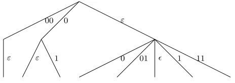
the binary strings that code the first branching direction. • Let the empty binary stringεbe the code of the branching direction M from the root of the tree, and then obtain the required coding of the rest of the subtree rooted at node(M)by applying the inductive hypothesis for trees of height at most h−1 and with at most` leaves. The lemma is illustrated, for an ordered tree of height2and with8 leaves, in Figures 1 and 2.
Note that the tree coding lemma implies the promised
(dlghe+ 1)dlg`eupper bound: everydlg`e-bounded adaptive
0
0
0 1
1
0 1 10 11 100
[image:5.612.60.285.47.132.2]10
Fig. 1. The branching directions are simply numbered in binary. For instance, the navigation path to the right-most leaf is(10,100), which uses5bits.
ε
00
ε 1
0
0 01 1 11
ε
Fig. 2. The same ordered tree is coded succinctly so that, in every navigation path, the total number of bits is at mostdlg 8e= 3(in this example, it happens to be at most2).
adaptive multi-counter. In Section IV we give more refined estimates of the size of the set
Sη,d = d/2
[
i=0
Bdlgηe,i
of dlgηe-bounded adaptive i-counters, where 0 ≤ i ≤d/2, which is the dominating term in the worst-case running time bounds of our lifting algorithm for solving parity games.
III. SUCCINCT PROGRESS MEASURES
A. Progress measures
For finite parity game graphs, a progress measure [13] is a mapping from the nvertices tod/2-tuples of non-negative integers (that also satisfies the so-called progressiveness condi-tions on an appropriate set of edges, as detailed below). Note that an alternative interpretation is that a progress measure maps every vertex to a leaf in an ordered treeT in which each of the at most nleaves has a navigation path of lengthd/2.
What are the conditions that such a mapping needs to satisfy to be a progress measure? For every priorityp∈ {1,2, . . . , d}, we obtain thep-truncation (rd−1, rd−3, . . . , r1)|p of the d/2
-tuple (rd−1, rd−3, . . . , r1) of non-negative integers, one per
each odd priority, by removing the components corresponding to all odd priorities i lower than p. For example, we have
(2,7,1,4)|8 = ε, (2,7,1,4)|5 = (2,7) and (2,7,1,4)|2 = (2,7,1). We compare tuples using the lexicographic order. We say that an edge (v, u)∈E isprogressive inµif
µ(v)|π(v)≥µ(u)|π(v),
and the inequality is strict when π(v) is odd. Finally, the mapping µ:V →T is aprogress measure[13] if:
• for every vertex owned by Even, some outgoing edge is progressive in µ, and
• for every vertex owned by Odd, every outgoing edge is progressive inµ.
B. Trimmed progress measures
Observe that the progressiveness condition of every edge
(v, u)∈E is formulated by referring to theπ(v)-truncations of the tuples labelling verticesv and u, so if the label of v is
(rd−1, rd−3, . . . , r1)then the components ri fori < π(v)are
superfluous for stating the condition. It is therefore reasonable to considertrimmed progress measuresthat label vertices with tuples(rd−1, rd−3, . . . , rk+2, rk)of length at mostd/2, rather
than insisting on all vertices having labels of length exactlyd/2. In the alternative interpretation discussed above, such a trimmed progress measure may then map some vertices to nodes in an ordered tree (of height at mostd/2) that are not leaves.
We clarify that if two tuples of different lengths are to be compared lexicographically, and if the shorter one is a prefix of the longer one, then the shorter one is defined to be lexicographically strictly smaller than the longer one For example, we have (1,0) < (1,0,3), but (1,0,3) <
(1,1). Moreover, truncations of tuples of length smaller than
d/2 are defined analogously; in particular, if p ≤ k then
(rd−1, rd−3, . . . , rk)|p= (rd−1, rd−3, . . . , rk).
C. Succinct progress measures
It is well known that existence of a progress measure is sufficient and necessary for existence of a winning strategy for Even from every starting vertex [6], [19], [13]. Our main contribution in this section is the observation (Lemma 4) that this is also true for existence of asuccinct progress measure, in which the ordered tree T is such that:
• finite binary strings ordered as in (1) are used as branching directions instead of non-negative integers, and
• for every navigation path, the sum of lengths of the binary strings used as branching directions is at mostdlgηe; or in other words, that every navigation path in T is adlgηe -bounded adaptive i-counter, for some i,0 ≤i≤d/2; recall that η is the number of vertices with an odd priority.
In succinct progress measures, truncations and lexicographic ordering of tuples, as well as progressiveness of edges, are defined analogously. Again, we clarify that if two tuples of different lengths are to be compared lexicographically, and if the shorter one is a prefix of the longer one, then the shorter one is defined to be lexicographically strictly smaller than the longer one. For example, we have (01, ε) <(01, ε,00), but
(01, ε,000)<(1000, ε). D. Sufficiency
Sufficiency does not require a new argument because the standard reasoning—for example as in [13, Proposition 4]— relies only on the ordered tree structure (through truncations), and not on what ordered set is used for the branching directions. We provide a proof here for completeness.
[image:5.612.59.291.173.255.2]Proof. Letµbe a succinct progress measure. Let Even use a positional strategy that only follows edges that are progressive inµ. Since every edge outgoing from vertices owned by Odd is also progressive inµ, it follows that only progressive edges will be used in every play consistent with the strategy. Therefore, in order to verify that the strategy is winning for Even, it suffices to prove that if all edges in a simple cycle are progressive inµ
then the cycle is even.
Let v1, v2, . . . , vk be a simple cycle in which all edges
(v1, v2),(v2, v3), . . . , (vk−1, vk), and (vk, v1)are progressive
in µ. For the sake of contradiction, suppose that the highest priority pthat occurs on the cycle is odd, and without loss of generality, letπ(v1) =p. By progressivity of all the edges on
the cycle, we have that
µ(v1)|p> µ(v2)|p≥ · · · ≥µ(vk)|p≥µ(v1)|p,
absurd.
E. Necessity
We prove necessity by first slightly strengthening the existence of the least progress measure result [13, Theorem 11], and then by applying the succinct tree coding lemma (Lemma 1).
As discussed earlier in this section, the range of a progress measure is the set of nodes in a tree of height d/2 and with at most n leaves. By applying Lemma 1 to this tree we may conclude that there is a tree coding in which branching directions on every navigation path use at most dlgne bits. This way we come short [sic] of satisfying our definition of a succinct progress measure: the definition allows us, on every path, to use at mostdlgηebits for branching directions, which may be strictly smaller than dlgne.
In order to overcome this hurdle, we first define the operation of a trimming of a progress measure. Let µ be a progress measure. We define thetrimmingµ↓ ofµas follows: for every vertex v, we let µ↓(v) be the longest prefix of µ(v) whose last component is not 0; in particular, if µ(v) is a sequence of 0s of length d/2 then µ↓(v) is the empty sequence. For convenience, we also define the inverse operation: if µ is a trimmed progress measure then for every vertex v, we let
µ↑(v)be the sequence of length d/2 obtained by adding an appropriate number (possibly none) of 0s at the end ofµ(v). Recall that by [13, Corollary 8] and by the proof of [13, Theorem 11] theleast progress measureµ∗ exists, where the relevant order on mappings from vertices to sequences of non-negative integers is pointwise lexicographic.
Lemma 3. The trimmingµ↓∗ of the least progress measureµ∗ is a trimmed progress measure and the ordered tree that it maps to has at mostη leaves.
Proof. Thatµ↓∗is a trimmed progress measure follows routinely fromµ∗ being a progress measure and from the definion of a trimmed progress measure.
We argue that for every leaf in the ordered tree T thatµ↓∗ maps into, there is a vertexv∈V with an odd priority, such
thatµ↓∗(v)is that leaf, which implies the other claim of the lemma.
Let λ= (rd−1, rd−3, . . . , rk)be a leaf in T. For the sake
of contradiction, assume that every vertex v ∈V such that
µ↓∗(v) =λhas an even priority. Note that—by the definition of a trimming—rk 6= 0, and hence—because µ∗ is the least progress measure—k > π(v). We define the mappingµλ as
follows:
• ifµ↓∗(v)6=λthenµλ(v) =µ↓∗(v); • ifµ↓∗(v) =λandk≥3 then
µλ(v) = (rd−1, . . . , rk+2, rk−1, n+ 1);
• ifµ↓∗(v) =λandk= 1then
µλ(v) = (rd−1, . . . , r3, r1−1).
We argue thatµλis a trimmed progress measure, and hence
µ↑λis a progress measure, which—becauseµ↑λis strictly smaller thanµ∗—duly contradicts the assumption thatµ∗was the least progress measure.
We only need to verify that every edge(v, u)∈E, such that
µ↓∗(v) =λ, and that is progressive in µ↓∗, is also progressive in µλ. This is straightforward if µ↓∗(u) = λ. Otherwise, we haveµ↓∗(v)|π(v)> µ↓∗(u)|π(v), which implies that
(rd−1, . . . , rk+2, rk−1)≥µ↓∗(u)|k. (2)
We now argue that µλ(v)|π(v) ≥µλ(u)|π(v) by considering
the following two cases.
• Ifπ(v) =k−1 then
µλ(v)|π(v)= (rd−1, . . . , rk+2, rk−1)≥µλ(u)|π(v),
where the inequality follows from (2). • Ifπ(v)< k−1 then
µλ(v)|π(v)= (rd−1, . . . , rk+2, rk−1, n+ 1)>
µ↓∗(u)|π(v)=µλ(u)|π(v),
where the inequality follows from (2) and because no component in the least progress measure µ∗ exceedsn.
Necessity now follows from applying the succinct coding lemma (Lemma 1) to the tree with at mostη leaves, which is obtained by Lemma 3.
Lemma 4 (Necessity). If there is a strategy for Even that is winning for her from every starting vertex, then there is a succinct progress measure.
IV. LIFTING ALGORITHM
winning strategy for player Odd in the original one. Note that the algorithm can be applied without any asymptotic penalty (and only cosmetic changes) to games in which vertices of priority0 are allowed, and hence the analysis of the algorithm applies to both the original game and its dual.
A. Algorithm design and correctness
Consider the following linearly ordered set of bounded adaptive multi-counters:
Sη,d = d/2
[
i=0
Bdlgηe,i,
and let Sη,d> denote the same set with an extra top element>. We extend the notion of succinct progress measures to mappings
µ:V →Sη,d> by:
• defining the truncations of >as >|p=>for allp;
• regarding edges (v, u)∈E such that µ(v) =µ(u) => andπ(v)is odd as progressive inµ.
For any mapping µ:V →Sη,d> and edge(v, w)∈E, let
lift(µ, v, w) be the least σ ∈ Sη,d> such that σ ≥ µ(v) and
(v, w)is progressive inµ[v7→σ]. For any vertexv, we define an operator Liftv on mappings V →Sη,d> as follows:
Liftv(µ)(u) =
=
µ(u) if u6=v,
min(v,w)∈Elift(µ, v, w) if Even owns u=v,
max(v,w)∈Elift(µ, v, w) if Odd owns u=v.
Theorem 5(Correctness of lifting algorithm).
1) The set of all mappingsV →Sη,d> ordered pointwise is a complete lattice.
2) Each operatorLiftv is inflationary and monotone.
3) From every µ : V → Sη,d> , every sequence of appli-cations of operatorsLiftv eventually reaches the least
simultaneous fixed point of allLiftv that is greater than
or equal toµ.
4) A mappingµ:V →Sη,d> is a simultaneous fixed point of all operatorsLiftv if and only if it is a succinct progress
measure.
5) If µ∗ is the least succinct progress measure, then{v :
µ∗(v)6=>}is the set of winning positions for Even, and any choice of edges progressive inµ∗, at least one going out of each vertex she owns, is her winning positional strategy.
Proof. 1) The partial order of all mappings V →Sη,d> is the pointwise product of n copies of the finite linear orderSη,d> .
2) We have inflation, i.e. Liftv(µ)(u) ≥ µ(u), by the
definitions ofLiftv(µ)(u)andlift(µ, v, w).
For monotonicity, supposingµ≤µ0, it suffices to show that, for every edge (v, w), we have lift(µ, v, w) ≤
lift(µ0, v, w). Writing σ0 forlift(µ0, v, w), we know that
1) Initialiseµ:V →Sη,d> so that it maps every vertexv ∈V to the bottom element inSη,d> , which is the empty sequence.
2) WhileLiftv(µ)6=µfor somev, updateµto becomeLiftv(µ).
3) Return the setWEven ={v : µ(v) 6=>} of winning positions
for Even, and her positional winning strategy that for every vertex
v∈WEven owned by Even picks an edge outgoing fromvthat is
progressive inµ.
TABLE I THE LIFTING ALGORITHM
σ0 ≥ µ0(v) ≥ µ(v). Also (v, w) is progressive in
µ0[v7→σ0], giving us that
σ0|π(v)≥µ0[v7→σ0](w)|π(v)≥µ[v7→σ0](w)|π(v)
and the first inequality is strict whenπ(v)is odd unless
µ0[v 7→ σ0](w) = >; but if µ0[v 7→ σ0](w) = > and
µ[v7→σ0](w)6=>then the second inequality is strict, so in any case(v, w)is progressive inµ[v7→σ0]. Therefore
lift(µ, v, w)≤σ0.
3) This holds for any family of inflationary monotone operators on a finite complete lattice. Consider any such maximal sequence fromµ. It is an upward chain from µ
to someµ∗which is a simultaneous fixed point of all the operators. For any µ0≥µwhich is also a simultaneous fixed point, a simple induction confirms that µ∗≤µ0. 4) Here we have a rewording of the definition of a succinct
progress measure, cf. Section III.
5) The set of winning positions for Even is contained in
{v : µ∗(v)6=>}by Lemma 4 becauseµ∗ is the least succinct progress measure.
Sinceµ∗ is a succinct progress measure, we have that, for every progressive edge (v, w), if µ∗(v) 6=> then
µ∗(w)6=>. It remains to apply Lemma 2 to the subgame consisting of the vertices{v : µ∗(v)6=>}, the chosen edges from vertices owned by Even, and all edges from vertices owned by Odd.
Note that the algorithm in Table I is a solution to both variants of the algorithmic problem of solving parity games: it finds the winning positions and produces a positional winning strategy for Even.
B. Algorithm analysis
The following lemma offers various estimates for the size of the set Sη,d of succinct adaptive multi-counters used in
the lifting algorithm in Table I, and which is the dominating factor in the worst-case upper bounds on the running time of the algorithm. A particular focus is the analysis pinpointing the range of the numbers of distinct prioritiesd(measured as functions of the numberη of vertices with an odd priority) in which the algorithm may cease to be polynomial-time. The “phase transition” occurs whend is logarithmic inη: if d=
o(logη)then the size ofSη,d isO η1+o(1)
, if d= Θ(logη)
then the size ofSη,d is bounded by a polynomial inη but its
degree depends on the constant hidden in the big-Θ, and if
Lemma 6 (Size of Sη,d).
1) |Sη,d| ≤2dlgηe dlgηed/+d/2 2+1.
2) Ifd=O(1)then|Sη,d|=O
ηlgd/2η.
3) Ifd/2 =dδlgηe, for some positive constantδ, then
|Sη,d|= Θ
ηlg(δ+1)+lg(eδ)+1.plogη, whereeδ = (1 + 1/δ)δ.
4) Ifd=o(logη)then|Sη,d|=O η1+o(1).
5) Ifd=O(logη)then |Sη,d| is bounded by a polynomial
inη.
6) Ifd=ω(logη)then |Sη,d| is superpolynomial inη and
|Sη,d|=O
dηlg(d/lgη)+1.45.
Proof. 1) There are 2dlgηe bit sequences of lengthdlgηe and for everyi,0≤i≤d/2, there are
dlgηe+i
i
=
dlgηe+i
dlgηe
distinct ways of distributing the numberdlgηe of bits toi+ 1 components (thei components in the succinct adaptive i-counter, and an extra one for the “unused” bits). By the “parallel summation” binomial identity, we obtain
d/2
X
i=0
dlgηe+i
i
=
dlgηe+d/2 + 1
d/2
.
In cases 3) and 6) below we analyse the simpler expressions dlgηd/e+2d/2
and dlgdηlge+ηed/2
, respectively,
instead of the above dlgηed/+d/2 2+1, in order to declutter calculations. This is justified because in each context the respective simpler expression is within a constant factor of the latter one, and hence the asymptotic results are not affected by the simplification.
2) This is easy to verify ford= 2andd= 4. Ifd≥6>2e
then for sufficiently largeη we have:
dlgηe+d/2 + 1
d/2
≤
(dlgηe+d/2 + 1)·(2e/d)d/2≤ dlgηed/2.
The former inequality always holds by the inequal-ity k` ≤ ek
`
`
applied to the binomial coefficient dlgηe+d/2+1
d/2
. The latter inequality holds for sufficiently large η because—by the assumption that d >2e—we have that2e/d <1, and hence the inequality holds for allη large enough that d/2 + 1≤(1−2e/d)dlgηe. 3) To avoid hassle, consider only the values ofηandδ, such
that bothlgη andδlgηare integers. Letd= 2δlgη and apply [1, Lemma 4.7.1] (reproduced as Lemma 9 in the Appendix) to the binomial coefficient
lgη+d/2
d/2
=
lgη+δlgη
δlgη
=
(δ+ 1) lgη
δlgη
,
obtaining
|Sη,d|= Θ η
(δ+1)H
δ δ+1
+1,p
logη
!
,
where H(p) =−plgp−(1−p) lg(1−p)is the bina-ry entropy function, defined for p ∈ [0,1]. A skilful combinator will be able to verify the identity
(δ+ 1)H
δ δ+ 1
= lg(δ+ 1) + lg(eδ).
4) This is a corollary of part 3) by observing that
limδ↓0eδ = 1and hence:
lim
δ↓0(lg(δ+ 1) + lg(eδ) + 1) = 1.
5) Again, this is a corollary of part 3) by observing that the expressionlg(δ+ 1) + lg(eδ) + 1isO(1)as a function
of η.
6) The first statement is a corollary of part 3) by observing that limδ→∞lg(δ+ 1) =∞ and limδ→∞eδ =e, and
hence:
lim
δ→∞(lg(δ+ 1) + lg(eδ) + 1) =∞. In order to prove the latter statement, note that
lg
dlgηe+d/2
dlgηe
≤
dlgηe ·hlg dlgηe+d/2
−lgdlgηe+ lgei=
dlgηe ·hlg (1 +o(1))d/2
−lgdlgηe+ lgei=
dlgηe ·
lgd−lgdlgηe+ lg(e/2) +o(1)
,
where the first inequality is obtained by taking thelgof both sides of the inequality k`
≤ ek `
`
applied to the binomial coefficient dlgdηlge+ηed/2
, and the second relation follows from the assumption that d=ω(logη). Then we have
|Sη,d|=O
2dlgηe· 1+lgd−lg lgη+lg(e/2)+o(1) =
O
2(1+lgη)· lgd−lg lgη+lge+o(1) =
Odηlg(d/lgη)+1.45 ,
where the latter holds because
2lgd−lg lgη+O(1)=O(d/lgη),
andlge+o(1)<1.4427for sufficiently largeη. Theorem 7 (Complexity of lifting algorithm).
1) If d=O(1) then the algorithm runs in time
Omηlgd/2+1η .
2) If d=o(logη)then the algorithm runs in time
3) Ifd≤2dδlgηe, for some positive constant δ, then the algorithm runs in time
Omηlg(δ+1)+lg(eδ)+1plogηlog logη . In particular, ifd≤ dlgηe, then the running time is
O mη2.38
.
4) Ifd=ω(logη)then the algorithm runs in time
Odmηlg(d/lgη)+1.45 .
The algorithm works in spaceO(nlogn·logd).
Proof. The work space requirement is dominated by the number of bits needed to store a single mappingµ:V →Sη,d> , which is at mostndlgηedlgde.
We claim that the Liftv operators can be implemented to
work in time O(deg(v)·logη·logd). It then follows, since the algorithm lifts each vertex at most |Sη,d| times, that its
running time is bounded by
O X
v∈V
deg(v)·logη·logd· |Sη,d|
!
=
O(mlogη·logd· |Sη,d|) .
From there, the various stated bounds are obtained by Lemma 6. For the last statement in part 3), note that if δ = 1/2 then
d≤ dlgηeimpliesd/2≤ dδlgηe, and
lg(δ+ 1) + lg(eδ) + 1 =
3
2lg 3<2.3775.
To establish the claim, it suffices to observe that every bounded adaptive multi-counter lift(µ, v, w) ∈ Sη,d> is com-putable in time O(logη ·logd). The computation is most involved when π(v)is odd and µ(v)|π(v)≤µ(w)|π(v) 6=>,
which imply that lift(µ, v, w) is the leastσ∈Sη,d> such that
σ|π(v) > µ(w)|π(v). Writing (sd−1, sd−3, . . . , sk+2, sk) for
µ(w), there are five cases:
• If k > π(v)and the total length of si is less than dlgηe,
then obtain σas
(sd−1, . . . , sk+2, sk,0· · ·0),
where the padding by0s is up to the total lengthdlgηe
of σ.
• Ifk≤π(v)and the total length ofsi fori≥π(v)is less
thandlgηe, then obtain σas
(sd−1, . . . , sπ(v)+2, sπ(v)10· · ·0),
where the padding by0s (if any) is up to the total length
dlgηeof σ.
• If the total length of si fori≥π(v)equals dlgηe,j is
the least odd priority such that sj 6= ε (in this case,
necessarily, j ≥π(v)), andsj is of the form s00 `
z }| {
1· · ·1
(where possibly`= 0), obtain σas
(sd−1, . . . , sj+4, sj+2, s0).
• If the total length ofsi for i≥π(v) equalsdlgηe,j is
the least odd priority such thatsj6=ε(again,j ≥π(v)),
sj is of the form `
z }| {
1· · ·1, andj < d−1, obtainσ as
sd−1, . . . , sj+4, sj+21
`−1
z }| {
0· · ·0
.
• Otherwise,σ=>.
Corollary 8 ([4]). Solving parity games is in FPT.
Proof. The algorithm runs in time
maxn2O(dlogd), O mη2.38o
.
ACKNOWLEDGEMENTS
We thank John Fearnley, Filip Mazowiecki, and Sven Schewe for helpful comments.
This research has been supported by the EPSRC grant EP/P020992/1 (Solving Parity Games in Theory and Practice).
REFERENCES
[1] R. B. Ash,Information Theory. Dover Publications, 1990.
[2] J. Bernet, D. Janin, and I. Walukiewicz, “Permissive strategies: from parity games to safety games,”Informatique Th´eorique et Applications, vol. 36, no. 3, pp. 261–275, 2002.
[3] A. Browne, E. M. Clarke, S. Jha, D. E. Long, and W. Marrero, “An improved algorithm for the evaluation of fixpoint expressions,”Theor.
Comput. Sci., vol. 178, no. 1–2, pp. 237–255, 1997.
[4] C. S. Calude, S. Jain, B. Khoussainov, W. Li, and F. Stephan, “Deciding parity games in quasipolynomial time,” inSTOC, 2017, to appear. [5] K. Chatterjee, M. Henzinger, and V. Loitzenbauer, “Improved algorithms
for one-pair and k-pair Streett objectives,” inLICS, 2015, pp. 269–280. [6] E. A. Emerson and C. S. Jutla, “Tree automata, mu-calculus and
determinacy,” inFOCS, 1991, pp. 368–377.
[7] E. A. Emerson, C. S. Jutla, and A. P. Sistla, “On model-checking for fragments ofµ-calculus,” inCAV, 1993, pp. 385–396.
[8] E. A. Emerson and C.-L. Lei, “Efficient model checking in fragments of the propositional mu-calculus (Extended abstract),” inLICS, 1986, pp. 267–278.
[9] J. Fearnley, S. Jain, S. Schewe, F. Stephan, and D. Wojtczak, “An ordered approach to solving parity games in quasi polynomial time and quasi linear space,” arXiv, March 2017,arxiv.org/abs/1703.01296v1. [10] H. Gimbert and R. Ibsen-Jensen, “A short proof of correctness of the quasi-polynomial time algorithm for parity games,” arXiv, February 2017, arxiv.org/abs/1702.01953v3.
[11] E. Gr¨adel, “Finite model theory and descriptive complexity,” inFinite
Model Theory and Its Applications. Springer, 2007.
[12] D. S. Johnson, “The NP-completeness column: Finding needles in haystacks,”ACM Trans. Algo., vol. 3, no. 2, 2007.
[13] M. Jurdzi´nski, “Small progress measures for solving parity games,” in
STACS, 2000, pp. 290–301.
[14] M. Jurdzi´nski and R. Lazi´c, “Succinct progress mea-sures for solving parity games,” arXiv, February 2017, arxiv.org/abs/1702.05051v1.
[15] M. Jurdzi´nski, M. Paterson, and U. Zwick, “A deterministic subexponen-tial algorithm for solving parity games,”SIAM J. Comp., vol. 38, no. 4, pp. 1519–1532, 2008.
[16] N. Klarlund, “Progress measures for complementation of omega-automata with applications to temporal logic,” inFOCS, 1991.
[17] ——, “The limit view of infinite computations,” inCONCUR, 1994, pp. 351–366.
[18] ——, “Progress measures, immediate determinacy, and a subset con-struction for tree automata,”Ann. Pure Appl. Logic, vol. 69, no. 2–3, pp. 243–268, 1994.
[19] N. Klarlund and D. Kozen, “Rabin measures,” Chicago Journal of
[20] O. Kupferman and M. Y. Vardi, “Weak alternating automata and tree automata emptiness,” inSTOC, 1998, pp. 224–233.
[21] M. Mnich, H. R¨oglin, and C. R¨osner, “New deterministic algorithms for solving parity games,” inLATIN, 2016, pp. 634–645.
[22] A. W. Mostowski, “Regular expressions for infinite trees and a standard form of automata,” inSymposium on Computation Theory, 1984, pp. 157–168.
[23] ——, “Games with forbidden positions,” Uniwersytet Gda´nski, Tech. Rep. 78, 1991.
[24] N. Piterman and A. Pnueli, “Faster solutions of Rabin and Streett games,” inLICS, 2006, pp. 275–284.
[25] S. Schewe, “Solving parity games in big steps,” inFSTTCS, 2007, pp. 449–460.
[26] H. Seidl, “Fast and simple nested fixpoints,”Inf. Process. Lett., vol. 59, no. 6, pp. 303–308, 1996.
[27] M. Y. Vardi, “Rank predicates vs. progress measures in concurrent-program verification,”Chicago Journal of Theoretical Computer Science, 1996, Article 1.
APPENDIX
A. Estimates for binomial coefficients
We outsource the challenge—and the tedium—of rigorously applying Stirling’s approximation to estimating binomial co-efficients k`, where`= Θ(k), to Ash [1]. The following is Lemma 4.7.1 from page 113 in his book.
Lemma 9 (Estimating binomial coefficients). If 0 < p < 1
and pk is an integer, then
2kH(p)
p
8p(1−p)k ≤
k
pk
≤ 2
kH(p)
p
2πp(1−p)k ,