Investigating interactions using solid state NMR: applications to biomolecular complexes

(1)

warwick.ac.uk/lib-publications

A Thesis Submitted for the Degree of PhD at the University of Warwick

Permanent WRAP URL:

http://wrap.warwick.ac.uk/

99641

Copyright and reuse:

This thesis is made available online and is protected by original copyright.

Please scroll down to view the document itself.

Please refer to the repository record for this item for information to help you to cite it.

Our policy information is available from the repository home page.

(2)

Investigating Interactions Using Solid State NMR:

Applications to Biomolecular Complexes

by

Carl Johan Wilhelm Öster

Thesis

Submitted to the University of Warwick

for the degree of

Doctor of Philosophy

Supervised by Dr. Józef R. Lewandowski

Department of Chemistry

(3)

List of Tables

TABLE1.1.PROPERTIES IMPORTANT FORNMR... 19

SITABLE2.1.15NR1RATES FORGB1FREEWITH VARYING CONCENTRATION OFGD(DTPA-BMA) ...87

SITABLE2.2.15NR1RATES FORGB1FREEWITH VARYING CONCENTRATION OFGD(DTPA-BMA) ...88

SITABLE2.3.15NR1RATES FORGB1CRYSTWITH0AND2MM GD(DTPA-BMA) ...89

SITABLE2.4.15NR1RATES FORGB1IGGWITH VARYING CONCENTRATIONS OFGD(DTPA-BMA) ... 90

SITABLE2.5.15NR1ΡRATES AT10KHZ NUTATION FREQUENCY FORGB1IGGWITH VARYING CONCENTRATIONS OF GD(DTPA-BMA) ... 91

SITABLE2.6.1HR1RATES FORGB1IGGWITH0AND100MM CU(EDTA)... 91

SITABLE2.7.EXPERIMENTAL15NSPREVALUES FORGB1FREE, GB1CRYSTANDGB1IGGAND1HSPRES FORGB1IGG...92

SITABLE2.8.PREDICTED15NSPREVALUES FORGB1FREE, GB1CRYST, GB1IGGANDGB1IN COMPLEX WITHIGG FRAGMENTS... 93

SITABLE2.9.PREDICTED1H PREVALUES FORGB1FREE, GB1IGGANDGB1IN COMPLEX WITHIGGFRAGMENTS... 95

SITABLE2.10.RELAXATION DELAYS USED AND TOTAL EXPERIMENTAL TIME FORR1MEASUREMENTS OFGB1FREEAND GB1CRYST...96

SITABLE2.11.RELAXATION DELAYS AND SPIN-LOCK LENGTHS AND TOTAL EXPERIMENTAL TIME USED FORR1ANDR1Ρ MEASUREMENTS OFGB1IGG...96

SITABLE2.12.RESULT OF FITTING OF EXPERIMENTALSPRES AGAINSTSPRES BACK-CALCULATED... 97

SITABLE2.13. PREDICTED1HSPRES FORGB1IGGBASED ON MODIFIED MODELS... 97

SITABLE2.14.PREDICTED1HSPRES FORGB1IGGBASED ON MODIFIED MODELS WITH AN ADDITIONAL INTERACTION SITE ...99

TABLE4.1.RESULTS FROMRDFITS FORGB1DIAANDGB1PRE...133

(5)

SITABLE4.2.RESULTS FROMRDFITS OF ALL RESIDUES COMBINED FORGB1DIA...154

SITABLE4.3.RESULTS FROMRD FITS OF THE Β REGION COMBINED FOR GB1DIA...155

SITABLE4.4.RESULTS FROMRD FITS OF THE Α REGION COMBINED FOR GB1DIA. ...155

SITABLE4.5.RESULTS FROMRDFITS OF INDIVIDUAL RESIDUES FORGB1PRE...156

SITABLE4.6.RESULTS FROMRDFITS OF ALL RESIDUES COMBINED FORGB1PRE...156

SITABLE4.7.RESULTS FROMRD FITS OF THE Β REGION COMBINED FOR GB1PRE...157

SITABLE4.8.RESULTS FROMRD FITS OF THE Α REGION COMBINED FOR GB1PRE...157

SITABLE4.9.RESULTS FROMRDFITS OF INDIVIDUAL RESIDUES FORGB1IN COMPLEX WITHIGG...158

SITABLE4.10.RESULTS FROMRDFITS OF ALL RESIDUES COMBINED FORGB1IN COMPLEX WITHIGG...158

SITABLE4.11.RESULTS FROMRDFITS OF RESIDUES EXPECTED TO BIND THEFC FRAGMENT OFIGGCOMBINED FORGB1 IN COMPLEX WITHIGG ...159

SITABLE4.12.RESULTS FROMRDFITS OF RESIDUES EXPECTED TO BIND THEFAB FRAGMENT OFIGGCOMBINED FORGB1 IN COMPLEX WITHIGG ...159

SITABLE4.13.NUMBER OF SPIN-LOCK LENGTHS,NUTATION FREQUENCIES AND TOTAL DURATION OF EACH EXPERIMENT. ...159

SITABLE4.14.STATISTICAL ANALYSIS OFRDFITS FOR ALL SAMPLES. ...159

SITABLE5.1. RESULTS FROM STRUCTURE CALCULATION OF[U-13C,15N]TEIXOBACTIN IN D38DPCMICELLES IN SOLUTION. ...174

SITABLE5.2. CHEMICAL SHIFTS FOR[U-13C,15N]TEIXOBACTIN IN D38DPCMICELLES,SOLUTIONNMRAT25 °C ...175

SITABLE5.3. CHEMICAL SHIFTS FOR[U-13C,15N]TEIXOBACTIN IN D38DPCMICELLES,SOLUTIONNMRAT37 °C...176

SITABLE5.4. CHEMICAL SHIFTS FOR[U13C15N]TEIXOBACTIN IN COMPLEX WITH LIPIDIIIN D38DPCMICELLES,SOLID STATENMRAT39 ± 2 °C...177

SITABLE5.5. RESULTS FROMKD FITS WITH A2:1RATIO OF TEIXOBACTIN:LIPID2...178

SITABLE5.6.COMPARISON OFKD FITS WITH DIFFERENT RATIOS OF TEIXOBACTIN:LIPIDII. ...180

List of Figures

FIGURE1.1.SCHEMATIC DRAWING OF PEPTIDOGLYCAN... 12

FIGURE1.2.PEPTIDOGLYCAN SYNTHESIS PATHWAY...14

FIGURE1.3.SCHEMATIC MODEL AND CHEMICAL STRUCTURE OFLIPIDII. ...16

FIGURE1.4.(ZEEMAN SPLITTING FOR A SPIN½NUCLEI ANDLARMOR PRECESSION AROUND THEB0FIELD. ...20

FIGURE1.5.CROSS POLARIZATION EXPERIMENT... 23

FIGURE1.6.MAGIC ANGLE SPINNING...25

FIGURE1.7.2D H-NCORRELATION SPECTRA FOR4DIFFERENT SAMPLES FIGURE1.8.EXAMPLES OF TIME SCALES OF DYNAMIC PROCESSES IN PROTEINS AND RELAXATION MEASUREMENTS TO OBTAIN INFORMATION ON THEM. ... 30

FIGURE1.9.SCHEMATIC DRAWING OF2DASSIGNMENT SPECTRA USED IN SOLUTIONNMR. ...35

FIGURE1.10.EXAMPLE STRIPS FROM SOLUTIONNMR 3DASSIGNMENT SPECTRA FOR[U-13C,15N]TEIXOBACTIN INDPC MICELLES. ...36

FIGURE1.11.EXAMPLE STRIPS FROM ASSIGNMENT SPECTRA OF[U-13C,15N]TEIXOBACTIN IN A SEDIMENTED COMPLEX WITH NATURAL ABUNDANCELIPIDIIIN DEUTERATEDDPCMICELLES...37

FIGURE1.12.STRUCTURE OFCYANALIBRARY ENTRY. ... 40

FIGURE1.13.STEPWISE EXPLANATION FOR HOW TO CREATECYANA LIBRARY ENTRIES... 42

FIGURE2.1.EXPERIMENTAL15NR1SOLVENTPRES FORGB1 ...59

FIGURE2.2.EXAMPLES OF LINEAR FITS FOR SPRES FORGB1IN A COMPLEX WITHIGG...62

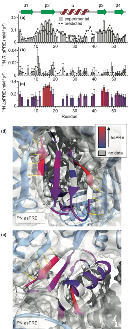
FIGURE2.3.15NΔSPRES FORGB1IGG... 64

(6)

FIGURE2.5.EXPERIMENTALΔSPRES VS.ΔSPRES PREDICTED FROMGB1:IGGMODELS...68

SIFIGURE2.1.COMPARISON BETWEEN EXPERIMENTAL AND PREDICTED15NSPRES FORGB1IN COMPLEX WITHIGG..83

SIFIGURE2.2. COMPARISON BETWEEN EXPERIMENTAL AND PREDICTED1HSPRES FORGB1FREE IN SOLUTION ANDGB1 IN COMPLEX WITHIGG ... 84

SIFIGURE2.3.EXAMPLES OF LINEAR FITS USED TO EXTRACT15NSPRES... 85

SIFIGURE2.4.MODEL OFGB1IN COMPLEX WITHIGGUSED FOR CALCULATIONS OF THEORETICAL SPRES... 86

SIFIGURE2.5.SECONDARY CHEMICAL SHIFTS FORGB1FREE IN SOLUTION ANDGB1IN COMPLEX WITHIGG...86

FIGURE3.1.15NR1 ANDR1ΡRELAXATION RATES FORGB1IN A COMPLEX WITHIGGAND IN AGB1CRYSTAL. ...103

FIGURE3.2.RESIDUES CLEARLY EXHIBITING CHEMICAL EXCHANGE ON THE ΜS TIME SCALE IN CRYSTALLINE GB1AND IN GB1IN COMPLEX WITHIGG. ...106

FIGURE3.3.15NR1ΡRATES FORGB1IN COMPLEX WITHIGGMEASURED AT VARYINGMASSPEED AND VISUALIZATION OF THE OVERALL3D GAFMOTION OFGB1IN THE COMPLEX WITHIGG ...109

FIGURES3.1.PULSE SEQUENCE USED FOR MEASURING15NR1ΡRATES IN THEGB1:IGGCOMPLEX...116

FIGURES3.2.ASSIGNED2D15N-1HSPECTRUM OF DEUTERATED(FULL-PROTONATED AT EXCHANGEABLE SITES) [U-13_C,15_N]GB1 IN COMPLEX WITH NATURAL ABUNDANCE FULL-LENGTH HUMANIGG...117

FIGURES3.3.ASSIGNED2D15N-1HSPECTRUM OF DEUTERATED(FULL-PROTONATED AT EXCHANGEABLE SITES) CRYSTALLINE[U-13C,15N]GB1. ...118

FIGURES3.4.SIMULATED15NR1ΡRATES FOR OVERALL ANISOTROPIC MOTION OFGB1ABOUT THREE DIFFERENT MOTIONAL AXES...119

FIGURES3.5.15NR1ΡRELAXATION DISPERSION CURVES MEASURED ON CRYSTALLINEGB1...122

FIGURES3.6.DIFFERENCES BETWEEN THE15NR1ΡRELAXATION RATES MEASURED AT2.5KHZ AND17KHZ SPIN-LOCK FIELDS FORGB1IN COMPLEX WITHIGG...123

FIGURES3.7.COMPARISON OF HELIX PACKING INGB1CRYSTAL ANDGB1IN COMPLEX WITHIGG...124

FIGURES3.8.COMPARISON OF15NR1ΡRATES MEASURED AT56AND39KHZ SPINNING FREQUENCIES MEASURED FOR CRYSTALLINEGB1AT10KHZ NUTATION FREQUENCY. ...127

FIGURE4.1.15NR1RELAXATION DISPERSION FOR CRYSTALLINEGB1...131

FIGURE4.2.15NR1RELAXATION DISPERSION PROFILES FORGB1IN COMPLEX WITHIGG...134

FIGURE4.3.MICROSECOND EXCHANGE IN CRYSTALLINEGB1ANDGB1IN A COMPLEX WITHIGG ...135

SIFIGURE4.1.RELAXATION DISPERSION PROFILES FORGB1DIAAT16.4 T...146

SIFIGURE4.2.RELAXATION DISPERSION PROFILES FORGB1DIAAT14.1 T. . ...147

SIFIGURE4.3.RELAXATION DISPERSION PROFILES FORGB1PREAT16.4 T. ...148

SIFIGURE4.4.RELAXATION DISPERSION PROFILES FORGB1PREAT14.1 T...149

SIFIGURE4.5.RELAXATION DISPERSION PROFILES FORGB1IN COMPLEX WITHIGG,WITH5MM GD(DTPA-BMA)AS PARAMAGNETIC RELAXATION ENHANCEMENT AGENT,MEASURED AT20 T. ...150

SIFIGURE4.6.RELAXATION DISPERSION PROFILES FORGB1IN COMPLEX WITHIGG,WITH2MM GD(DTPA-BMA)AS PARAMAGNETIC RELAXATION ENHANCEMENT AGENT,MEASURED AT16.4 T. ...151

SIFIGURE4.7.GB1STRUCTURES WITH RESIDUES COLORED BASED ON RELAXATION DISPERSION PROFILES OFGB1DIAAND GB1PRE. ...152

SIFIGURE4.8.GB1STRUCTURES WITH RESIDUES COLORED BASED ON RELAXATION DISPERSION PROFILES OFGB1IN COMPLEX WITHIGG.. ...153

FIGURE5.1.COMPARISON BETWEEN A SOLUTIONNMRSTRUCTURE OF TEIXOBACTIN INDPCMICELLES WITH A CRYSTAL STRUCTURE OF TEIXOBACTIN ANALOGUEAC-Δ1-5ARG10-TEIXOBACTIN ANDRESULTS FROMKD FITS OF A2:1 TEIXOBACTIN:LIPIDIIBINDING MODE...163

FIGURE5.2. COMAPRISON OF CHEMICAL SHIFTS BETWEEN TEIXOBACTIN IN SOLUTION AND TEIXOBACTIN IN COMPLEX WITH LIPIDIIIN SOLID STATE. ...165

SIFIGURE5.1.1H-15NSOLID STATENMRSPECTRUM OF[U,13C,15N]TEIXOBACTIN IN COMPLEX WITH NATURAL ABUNDANCE LIPIDIIIN D38DPCMICELLES...173

(7)

Acknowledgements

During my PhD I have had the opportunity to work together with many great scientists, both at the University of Warwick and externally and I am grateful for everything I have learned and all the help I have got. First I would like to thank Józef Lewandowski for his great supervision. I consider myself lucky to have had a dedicated supervisor who was always available for discussion. I would also like to thank the other members of the Lewandowski group especially Jonathan Lamley for teaching me how to run solid state NMR experiments and Simone Kosol for teaching me how to produce isotope labelled proteins, helping me with solution NMR experiments and for great collaborations on the solvent PRE project. Also thanks to Angelo Gallo for help with solution NMR and Trent Franks for help with pulse programs for solid state NMR experiments.

(8)

Declarations

All experimental chapters are results of collaborations. My contributions to the work are stated in this section. My supervisor, Józef Lewandowski, was of course involved in all the projects and made significant

contributions to all aspects from planning experiments to analysing data and writing the manuscripts. Chapter 2 has been accepted for publication in Journal of the American Chemical Society. In chapter 2, I produced the isotopically labelled GB1 together with Simone Kosol. I acquired,

processed and analysed all the solid state NMR experiments except for the 1_H _R

1measurements with 100 mM CuEDTA which was acquired by

Jonathan Lamley. I have also proposed a new parameter called difference

solvent paramagnetic relaxation enhancement (ΔsPRE) and theoretical

treatment of the data for identifying protein-protein interactions based on the difference in solvent accessibility measured in isolated protein in solution and in a sample with protein-protein interactions in solid state. Simone Kosol measured the solution NMR experiments and Christoph Hartlmüller and Tobias Madl performed the PRE predictions. Chapter 3 is published in Angewandte Chemie and was led by a previous PhD student in our group, Jonathan Lamley. I was involved originally by assisting in packing solid state NMR rotors and acquiring data as part of my training. I also assisted in data analysis, making figures and editing the

manuscript. After Jonathan left the group I performed most of the additional experiments and data analysis required for publication. My main contributions to the paper were the site specific 15_N _R

1 measurements at varying MAS speeds and site specific 15_N _R 1

measurements for GB1 in the complex with IgG. An early version of this manuscript was included in Jonathan Lamley’s PhD thesis. However, the final version is significantly different and includes more data that I

acquired. The isotopically labelled GB1 used in chapter 3 was provided by Stephan Grzesiek and co-workers at the University of Basel. In chapters 4 and 5 I have conducted all the experiments and data analysis. The isotopically labelled GB1 used in chapter 4 was from the same batch that I produced together with Simone Kosol, used in chapter 2. The

(9)

University and Dallas Hughes at Novobiotics (US). Lipid II was provided by the David Roper and Christopher Dowson groups at the School of Life Sciences, University of Warwick. In order to perform structure

calculations of molecules with non-proteinogenic residues I have

produced a large library for the molecular dynamics software CYANA that was used in the structure calculations in chapter 5. This library can deal with modified amino acid containing standard peptide bonds but also residues containing other types of bonds, such as glycosidic bonds between sugar molecules. The 0.81 mm probes used in chapters 2 (for 850 MHz spectrometer) and 5 (for 600 MHz spectrometer) were

developed by Ago Samoson and co-workers in Estonia. The 0.81 mm probe for the 600 MHz spectrometer belongs to our group and was an experimental probe in which development our group was involved. I have spent a lot of time optimising the sample preparations, and general

procedures for running of this probe. For all chapters, except chapter 3, I wrote the original manuscripts, which were subsequently edited

collaboratively with the co-workers. As will be made clear in the thesis I have during my PhD gained experience in preparing samples for and running NMR experiments, mainly in the solid state but also in solution, to investigate structures and dynamics of proteins, protein complexes, small peptides, cell wall fragments and complexes of peptides and cell wall fragments. I have also learned how to calculate 3D structures of biomolecules based on NMR data, and gained further understanding in how the structure calculation software work to be able to incorporate non-proteinogenic residues. During my PhD I also contributed the following published papers;

Solid-State NMR of a Protein in a Precipitated Complex with a Full-Length Antibody, Lamley, J.M., Iuga, D., Öster, C., Sass, H.J., Rogowski, M., Oss, A., Past, J., Reinhold, A., Grzesiek, S., Samoson, A., Lewandowski, J.R. J. Am. Chem. Soc. 2014136 (48):16800–16806.

Protein residue linking in a single spectrum for magic-angle spinning NMR assignment, Andreas LB, Stanek J, Le Marchand T, Bertarello A, Cala-De

(10)

S, Engelke F, Felli IC, Pierattelli R, Dixon NE, Emsley

L, Herrmann T, Pintacuda G. J Biomol NMR 2015 62 (3) 253-61

(11)

Abstract

(12)

1. Introduction

The following chapter provides theoretical basis for understanding the experimental chapters 2-5. Chapter 2 discusses characterisation of protein – protein interfaces using solvent paramagnetic relaxation enhancements. Chapters 3-4 concern protein dynamics in large protein complexes and chapter 5 interactions between an antibiotic and a bacterial cell wall precursor. The common theme in all the experimental chapters is that they include the use of solid state NMR to obtain vital information about interactions in biomolecular complexes. In chapters 2-4 the complex studied is a > 300 kDa protein – antibody complex formed between the B1 domain of bacterial Protein G (GB1) and human immunoglobulin G (IgG), in chapter 5 it is the complex formed between an antibiotic, teixobactin, and a cell wall precursor, lipid II. This introduction includes information regarding bacterial cell walls, solid state NMR of biomolecules and structure determination by NMR in solution and in solid state. More specific information related to the experimental work conducted is provided in each experimental chapter. The introduction gives more general descriptions of important information that is not included in the experimental chapters, i.e. information that is vital to understand how the results were obtained but not suitable for inclusion in publications. The original aim of my PhD project was to obtain structural information on bacterial cell walls or on cell wall fragments involved in the cell wall synthesis and how antibiotics can inhibit the synthesis of cell walls. In order to achieve this I worked a lot on methods development for solid state NMR approaches on large complexes, e.g. the GB1:IgG complex.

1.1 GB1:IgG complex

The B1 domain of Protein G (GB1) has been used as a model protein in solution and solid state NMR method developments for decades due to its stable fold and large yields in protein production. The solution NMR

structure of GB1 was solved already in 19911_{. For solid state NMR}

(13)

leading to that it was one of the first protein structures solved by solid state NMR2–4_{. However, there is also a biological interest for GB1; the}

binding to IgG antibodies. Protein G is produced by group G and C

streptococci as a part of the bacterial defence strategy against antibodies that enables bacteria to escape detection by the host immune system.5

The high affinity between GB1 and IgG is commonly exploited in

numerous biotechnological applications such as immunosorbent assays or affinity purification of antibodies. IgG antibodies are used in a range of therapeutic applications such as cancer treatment and treatments of infectious diseases. Antibody-based drugs are one of the fastest growing classes of protein therapeutics and of these unmodified IgG antibodies are the most common.6 _{Solution NMR and X-Ray crystallography has}

been used to study interactions between domains of Protein G and fragments of IgG but only with solid state NMR is it possible to investigate interactions with full length IgG. See chapter 2 for more details on interactions between GB1 and IgG and chapters 3-4 for details on the dynamics of GB1 in complex with IgG.

1.2 Antimicrobial resistance

Antimicrobial resistance (AMR) is a global threat resulting in hundreds of thousands of deaths each year. At the same time the development of new antibiotics has been slow and there is an urgent need for new antibiotics that can tackle bacteria that have acquired resistance against current last resort antibiotics. If these issues are not tackled the estimated deaths caused by AMR are expected to overtake cancer and according to the O’Neill report7 _{10 million people will die each year from}

AMR in 2050. Strategies for obtaining new antimicrobial agents include identifying good targets, which are conserved between different strains of bacteria and not present in human cells. Such a target is the cell wall building block lipid II, which is considered in the work presented here.

1.2.1 Peptidoglycan

(14)

withstanding turgor pressure. If the peptidoglycan is damaged or if the synthesis of peptidoglycan is interrupted the cell will be destroyed. This has of course been widely utilized in antibiotics design. In fact penicillin, which was discovered by Alexander Fleming in the famous accidental growth of mould incident8_{, is inhibiting the synthesis of peptidoglycan in}

bacteria. Although it took around 35 years from the initial discovery until it was discovered that penicillin works by inhibiting transpeptidation (see Fig.1.2) in the peptidoglycan synthesis9,10_{. Peptidoglycan is also}

responsible for keeping a certain cell shape and functions as a scaffold for anchoring other cell envelope components such as proteins and teichoic acids. It is closely involved in cell division and cell growth.11

Figure 1.1 shows a schematic drawing of peptidoglycan.

Figure 1.1.Schematic drawing of peptidoglycan. Red lines indicate peptide links connecting glycan strands.

Peptidoglycan is composed of linear glycan strands that are connected through peptide links (red lines in Fig. 1.1). The glycan strands consist of alternating acetylglucosamine (NAG, green in Fig. 1.1) and

N-acetylmuramic acid (NAM, orange in Fig. 1.1) connected through β-1-4

bonds.11 _{The glycan strands can be modified in different ways;}

N-deacetylation, N-glycolylation, O-acetylation, δ-lactam formation,

attachment of surface polymers and formation of 1-6 anhydro ring.12

(15)

modifications is not very well understood, even though some enzymes responsible for modifications have been identified.12

The peptide links are formed between peptide stems situated on the NAM residue of each disaccharide. The peptide stem varies between

different species but the most common is

L-Ala-D-Glu-DAP(diaminopimelic acid)/L-Lys-D-Ala-D-Ala. Variations in this peptide sequence can result in resistance against antibiotics, which is the case for bacteria that have obtained resistance against vancomycin (discussed below in section 1.1.2). The peptide link is usually established between the carboxyl group in the amino acid at position 4 and the amino group in the diamino acid at position 3.11 _{In most gram negative bacteria it is a}

direct cross-link and in most gram positive bacteria it has an interpeptide bridge. Two of the most studied bacteria when it comes to peptidoglycan are the gram negative Escherichia coli and the gram positive

Staphylococcus aureus. These two differ in peptide cross links as E. coli

has a direct 3-4 cross link while S. aureus has a 3-4 pentaglycine bridge. The length of the interpeptide bridge can vary between 1 and 7 amino acids and there are many different amino acids present in different bacteria. Also the degree of cross-linkage varies. In E. coli approximately 20% of the peptide stems are involved in cross-linkage whereas in S. aureus it is more than 90%.11 _{All these different variations in}

peptidoglycan structure may be important for how bacteria respond to antimicrobial agents and more understanding of peptidoglycan and the synthesis of peptidoglycan is important for the development of new antibiotics.

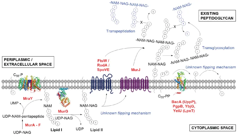
Figure 1.2 shows a schematic drawing of the peptidoglycan biosynthesis pathway adapted from a recent review by Teo and Roper13_.

(16)

[image:16.595.112.527.72.306.2]

Figure 1.2.Peptidoglycan synthesis pathway13

Lipid II consists of the general building blocks of peptidoglycan (shown in figure 1.1), linked through a pyrophosphate group and a carrier lipid (undecaprenyl pyrophosphate) attached to the membrane (the chemical structure of lipid II is shown in figure 1.3).

1.2.2 Antibiotics binding to Lipid II

Antibiotics that inhibit the cell wall synthesis are the most popular type of antibiotics and, as mentioned before, lipid II is an excellent target to focus on. There are many different types of lipid II binders including; glycopeptides, defensins, lantibiotics and nonribosomally synthesised peptides (e.g depsipeptides), recently reviewed by Oppedisjk et al14_.

(17)

being formed leading to almost a 1000 fold decrease in affinity15_{. This}

substitution has been seen in Lactobacillus casei naturally and in Enterococci with acquired resistance to vancomycin11_{. Since vancomycin}

(18)

[image:18.595.123.509.72.363.2]

Figure 1.3.(a) Schematic model of lipid II with binding sites for different types of antibiotics indicated. (b) chemical structure of lipid II. The lipid tail is represented by C55as it contains 55 carbons.

A novel lipid II binding mode was identified for nisin from solution NMR measurements of a nisin – lipid II complex16_{. In this binding mode a}

pyrophosphate cage is formed by intermolecular hydrogen bonds between backbone amides of nisin in the N-terminus lanthionine ring and the pyrophosphate group of lipid II. The N-terminal lanthionine ring is conserved in many lantibiotics and it is likely that the same binding mode occurs in other lantibiotics. A lanthionine ring is formed by bonds

between side-chains of modified alanines where the β-carbons are

(19)

transglycosylation. Class B lantibiotics undergo substantial conformational changes in different environments and when binding lipid II. This behaviour was shown in an NMR study where conformational changes were detected when the sample solution was changed from a

methanol/water solution to a membrane environment

(dodecylphophocholine (DPC) micelles) and then again when Lipid II was present17_{. Such conformational changes could be important for how the}

antibiotic enters the cell and reaches the membrane where lipid II is located.

An example of an interesting depsipeptide is ramoplanin, which is a cyclic lipoglycodepsipeptide. Ramoplanin inhibits peptidoglycan synthesis by blocking transglycosylation upon binding to Lipid II. The mode of action of ramoplanin seems to be similar as mersacidine, in both cases they accumulate cell wall precursors inhibiting the formation of peptidoglycan, and even though the chemical structure is very different between the two antibiotics their 3D structures are very similar and they both undergo conformational changes upon binding to lipid II18_.

Defensins are found in mammals, invertebrates and plants where they function as host defence peptides. A very interesting defensin is plectasin19_{, which was shown by NMR to form hydrogen bonds with the}

pyrophosphate of lipid II and blocking synthesis of peptidoglycan in a similar way as mersacidine and ramoplanin. In that study several other defensins binding lipid II were isolated from fungi, maggots and mussels

20_.

In many structural studies of antibiotics NMR has been an indispensable technique. However, in some studies it was noted that antibiotics – lipid II complexes form large soluble aggregates, making solution NMR unusable. In the case of ramoplanin it formed fibrillar structures18 _that

(20)

size dependent tumbling of molecules is not present. This study is presented in chapter 5.

1.3 NMR

The main technique used in the work presented in this thesis is NMR. Depending on the sample investigated the experiments were performed in solution or in solid state. Most of the samples were not suitable for solution NMR due to size implications but in the cases where applicable, solution NMR gave important information: It was used to obtain solvent accessibility for isolated GB1 in chapter 2 and to solve the 3D structure of teixobactin in membrane mimics in chapter 5. This section is mostly focused on solid state NMR, but the information is valid for solution NMR as well and important aspects where the techniques differ are pointed out.

1.3.1 Basic theory

In this section a few important theoretical aspects of NMR will be briefly discussed. The NMR interactions are described by quantum mechanics and it is beyond the scope of this thesis to go into a full description of the physics required to explain it properly. Some important theoretical aspects will be introduced but the explanations will be left out. This section is based on information that can be found in the NMR text books written by Malcolm H. Levitt21_{, James Keeler}22_{, Melinda J. Duer}23_{, Gordon}

S. Rule and Kevin T. Hitchens24_.

(21)

Table 1.1.Properties important for NMR of different isotopes of the most common nuclei in proteins.

Nucleus Spin Abundance (%) γ(MHz / T)

1_H _½ _99.98 _42.57697

2_H ₁ _0.0015 _6.535857

3_H _½ ₀ _45.41486

13_C _½ _1.108 _10.70842

14_N ₁ _99.63 _3.077738

15_N _½ _0.37 _-4.31628

17_O _⁵⁄₂ _0.037 _-5.77398

For hydrogen the most abundant isotope is 1_{H, which also has the largest}

gyromagnetic ratio (γ) of all nuclei used for NMR. 3_{H has a larger} _γ_{, but it}

is radioactive and not naturally abundant so it is not often used in NMR. For carbon, where the most abundant isotope is 12_{C, which is a spin 0}

isotope, typically it is necessary to introduce 13_{C (natural abundance} 13_C

can be used for smaller compounds) and 15_{N is introduced instead of} 14_N

(which is quadrupolar and can be measured but is generally not used in proteins) for NMR applications. Oxygen would be very useful but since

16_{O is spin 0 and the NMR active} 17_{O is spin 5/2 and hence has a}

quadrupolar moment it is not often used in protein NMR (though it is still an active area of method development).

The first interaction in NMR that needs to be considered when a sample is put in a static magnetic field (B0) is called the Zeeman interaction, which

describes how spins are split into quantum states with different energy levels (Figure 1.4a). For nuclei with spin I the number of energy levels is 2I+1. Spin ½ nuclei have then two energy levels, generally called Eα and

Eβ, where the difference in energy between the two states is defined as

the Larmor frequency:

= = × (1.1)

in Hz, γ is the gyromagnetic ratio (rad s-1 _T-1_{) and} _B

0 the static magnetic

field (T). The 2π is used to convert from rad s-1 _{to Hz. The spins are said}

to precess around the B0 field at the Larmor frequency (figure 1.4b).

(22)

The population ratio between the energy levels is described by Boltzmann distribution:

= ħ (1.2)

where ħ is Plancks constant divided by 2π, k is the Boltzmann constant andT is the temperature.

Figure 1.4.(a) Zeeman splitting for a spin ½ nuclei. The difference between the energy levels is the Larmor frequency. (b) Larmor precession around theB0field.

The Boltzmann distribution is important since the NMR signal partly depends on that the populations of the energy levels are different and the quantity of the difference can be changed by changing the gyromagnetic ratio, the B0 field and the temperature. Higher magnetic

field gives higher signal, higher gyromagnetic ratio gives higher signal and lower temperature gives higher signal, although for proteins there is normally not much room for changing the temperature to make any difference.

In a one pulse experiment a π/2 radiofrequency pulse is applied at the

Larmor frequency of the nuclei of interest with a certain nutation frequency

= × (1.3)

creating a local magnetic field B1. The spins will be rotated from the

(23)

induction decay (FID). The FID is then Fourier transformed into a time domain axis and plotted as intensity versus frequency.

Before moving on to experiments correlating different nuclei a few more interactions need to be introduced. So far the interactions (described by Hamiltonians in quantum mechanics) have been external; interactions between the magnetic field and the spins and interactions between radiofrequency pulses and the spins, but there are also internal interactions. The internal Hamiltonians are interactions of spins with the local electronic environment (chemical shift), with each other (dipolar and scalar couplings) and with electric field gradients (quadrupolar couplings). For spin ½ nuclei, which are considered in all experiments here, no quadrupolar interactions are present. The internal interactions can have parts that are isotropic (independent of orientation with respect to B0) and anisotropic (dependent of orientation with respect to B0).

Dipolar couplings are anisotropic and consist of both homonuclear and heteronuclear couplings in a sample with more than one nucleus. To fully describe the dipolar couplings it would be necessary to involve quantum mechanics, but for the purpose of this thesis it is sufficient to present the dipolar couplings as:

∝ (3 cos − 1) (1.4)

where r is the distance between the coupled spins and θ is the angle formed between the spins and the B0field. The chemical shift depends on

the Larmor frequency and chemical shielding based on the electronic environment around the spin. The chemical shift can be described as:

= (1 − ) (1.5)

where σ is the chemical shielding. The isotropic chemical shift (i.e. the component of chemical shift that is independent of the orientation with respect to B0) is simply the Larmor frequency determined from the local

(24)

couplings is proportional to the second Legendre polynomial ½(3cos2_θ _–

1). Scalar couplings, or J-couplings as they are normally referred to, are isotropic and give rise to J-splittings in NMR spectra. Since they are much weaker than dipolar couplings and chemical shift anisotropy the line widths reachable in solid state NMR typically are broader than the J-splittings so they are often ignored. However, with recent methodological advances and improvements in resolution J-couplings receive more attention in the solid state.

Line broadening is caused by the effect of anisotropic interactions on the

T2 relaxation time, which represents the loss of coherence in the

transverse plane due to spin-spin interactions. Further information on relaxation is given in section 1.3.3. There are two main ways of removing unwanted broadening caused by the interactions described above; rotating the sample and decoupling. In solution NMR the molecules tumble freely and sample all orientations leading to that anisotropic interactions are averaged to 0. J-couplings, which are isotropic, are still present but can be removed by decoupling. Heteronuclear J-couplings are weak and easily removed by applying a weak radio frequency field on, for example, the 13_{C channel during} 1_{H detection. Homonuclear}

couplings, however, are more complicated to remove and lead to J-splitting normally seen in solution NMR experiments. As mentioned above, in solid state NMR the lines are often not sufficiently narrow to observe J-splittings. To remove anisotropic interactions in solid state NMR the sample is mechanically rotated at the magic angle (θ = 54.74°), where ½(3cos2_θ _{– 1) = 0. For the magic angle spinning (MAS)}25,26 _to

efficiently average out the anisotropic interaction the spinning speed needs to be much faster than the strength of the interaction (in Hz).

As mentioned above the Boltzmann distribution is important for the sensitivity of an NMR experiment, the increase in γ to increase the sensitivity is taken advantage of in the cross–polarization (CP)27

experiment, in solid state NMR, where magnetization from the higher γ

nuclei, often 1_{H, can be transferred to lower} _γ _{nuclei (}13_{C or} 15_{N in}

(25)

CP experiment and what happens to the magnetization during the experiment.

Figure 1.5. Cross polarization experiment. Left, block diagram of the pulse sequence. Right, magnetization transfer showed on xyz coordinates.

First a π/2 pulse is applied to the 1_{H channel, which causes the}

magnetization to go into the xy plane. In this example the pulse was applied about the y axis leading to magnetization along x. The CP transfer is made up of spin-lock pulses at both channels simultaneously causing the magnetization to precess around x at the same nutation frequency for both nuclei as long as the pulse is on. Now the strong heteronuclear dipolar couplings will cause magnetization to transfer between the excited 1_{H spins and the} 13_{C spins. Once the pulse is turned}

off the spins will precess around the x-axis at the Larmor frequency and the FID can be recorded on the 13_{C channel, while heteronuclear}

decoupling is applied to the 1_{H channel. For the transfer to work the}

nutation frequencies need to be equal for both channels so that the Hartmann – Hahn condition is fulfilled:

= (1.6)

This is valid in static samples, but when MAS is employed making the dipolar couplings time dependent the Hartmann-Hahn matching condition becomes:

± = , = 1,2 (1.7)

If the magnetization transfer would be 100% efficient the signal could be increased by a factor of γ1/γ2, compared to an experiment with direct

(26)

13_{C and 10 if} _γ

1 is 1H, γ2 is 15N. CP experiments can also be repeated

quicker since the repetition delay depends on the T1 relaxation time (see

section 1.3.3) of the excited nuclei and the spins need to return to equilibrium before the next experiment can be started. T1s for protons

are much shorter than T1s for lower gamma nuclei (e.g 13C and 15N)

leading to higher signal to noise ratio in the same time (signal to noise

ratio increases by √n, where n = number of repetitions).

In most NMR experiments it is desirable to obtain as narrow lines as possible, especially in protein NMR since the spectra typically contain many signals and if the peaks are too broad it is difficult to assign which peaks belong to which atom in the protein. To achieve narrow lines when using MAS it is important that the rotor angle is set properly. There are several options for what type of sample is used to set the angle depending on the spinning speed. The probes that were used in this work were 1.3 mm probes that have operational MAS speeds up to 60 kHz and 0.81 mm probes with operational MAS speeds up to 100 kHz. The probe sizes refer to the outer diameter of the rotors used in the specific probe. In this fast spinning regime the magic angle can be set using a [13_C’]

labelled alanine sample since the spinning speeds are much higher than the strengths of the anisotropic interactions in this sample. Figure 1.6a shows a schematic drawing of MAS and 1.6b shows CP spectra of [13_{C’]alanine obtained at 60 kHz MAS with the magic angle slightly off,}

anisotropic interactions causing line broadening (red) and the magic angle set correctly, anisotropic interactions sufficiently averaged out (blue). Not only is the peak narrower when the magic angle is set properly, the maximum intensity is also higher. Overall, the line width also depends on inhomogenous broadening, which depends on how well the sample is recrystallised. In our laboratory, for a well-crystallised [13_{C’]alanine sample the} 13_{C line width in the case where the magic angle}

(27)

Figure 1.6. Magic angle spinning. (a) NMR rotor with the angle towards the static magnetic field indicated. (b)1H –13C CP spectra of [13C’]alanine with the magic angle set correctly (blue line) and the magic angle set incorrectly (red line).

It can be noted in the spectra in Figure 1.6b that the chemical shift (δ) is

presented in ppm, parts per million. This is the general convention of how chemical shifts are presented as spectra can then easily be compared between experiments acquired at different B0 fields. The

chemical shifts in ppm are calculated as:

= × 10 (1.8)

where is the chemical shift of a reference material. In protein NMR the reference used is often DSS (2,2-dimethyl-2-silapentane-5-sulfonic acid) as it is soluble in aqueous solutions and does not interact with biological samples. It can be put into the rotor in solid state NMR or the sample tube in solution NMR together with the protein sample. The 1_H

chemical shift of DSS is only very slightly affected by the temperature in the sample (at least in the range of temperatures suitable in protein NMR) further making it suitable as a reference. Referencing is then easily done by recording a 1 pulse 1_{H experiment and setting the peak}

originating from the DSS sample to 0 ppm. References for 13_{C and} 15_N

can then be calculated indirectly from the 1_{H reference by using IUPAC}

recommended ratios28,29_.

1.3.2 Biological assemblies in NMR

(28)

However, large molecules tumble slowly, which results in efficient transverse relaxation causing severe broadening of the lines so that no or little information can be extracted from the spectra. Solution NMR therefore suffers from strong size limitations for larger molecules (>40 kDa). The size of molecules accessible to solution NMR can be sometimes extended by using a number of methodological tricks such as deuteration and TROSY type techniques but it is difficult in general. X-ray crystallography requires good quality diffracting crystals and membrane proteins or molecules with large internal motions or highly flexible domains are notoriously difficult to crystallize. With solid state NMR it is in principle possible to study any kind of biological molecules and assemblies independent of the size and there are several different ways of preparing the samples before they are put into the NMR rotors. Very good resolution is achieved from microcrystalline proteins, without the need for the same kind of quality crystals as in X-ray crystallography. No long-range order is required, however the sample needs to be homogenous since inhomogeneous broadening can severely limit the possibility of obtaining good quality spectra. Samples can also be precipitated, sedimented by ultracentrifugation, freeze dried, or analysed in the form of fibrils. In many cases proteins packed into NMR rotors can be stable for months and even years.

Solid state NMR has become an important technique for studying protein assemblies30–39_{. The main areas of interest for large complexes or}

assemblies are fibrils, virus capsids and membrane proteins. Recent developments in solid state NMR of membrane proteins have been reviewed by Ladizhansky40_{. Quinn and Polenova}41 _{have reviewed}

developments in solid state NMR on structure and dynamics of protein complexes and other biomolecular assemblies (e.g. virus capsids). Of specific interest to this thesis is the use of proton detection to study protein complexes and biomolecular assemblies. Regarding membrane proteins and fibrils it was first shown by Linser et al. that high quality spectra could be obtained using proton detection of Alzheimer’s disease

β-amyloid peptide (fibrils) and membrane proteins.42 _{Further work in}

(29)

and structural information using proton detection on these types of complicated samples as shown for example in ref. 43. Recent developments of fast spinning MAS probes and high field NMR magnets enable high resolution site specific information requiring only a few nanomoles of labelled material (e.g. as demonstrated for GB1 in complex with IgG36_).

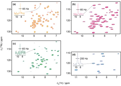
In the work presented in this thesis three different types of sample preparations were used; microcrystalline protein, precipitated protein – protein complex and a sedimented sample of cell wall bound antibiotic. Figure 1.7 shows 1_H-15_{N correlation spectra of samples prepared using}

these different methods, including both perdeuterated crystalline

[U-13_C,15_{N]GB1 with 100% of exchangeable protons back-exchanged (a) and}

fully protonated crystalline [U-13_C,15_{N]GB1 (b). Figure 1.7c shows a}

spectrum of 100% back-exchanged perdeuterated [U-13_C,15_{N]GB1 in a}

precipitated complex with full length natural abundance human Immunoglobulin G (IgG) antibody and (d) shows a sedimented complex of [U-13_C,15_{N]teixobactin with natural abundance lipid II in deuterated}

dodecylphosphocholine (DPC) micelles. All solid state experiments considered in this thesis are acquired with proton detection. For proton detected experiments it is important to use fast MAS as strong 1_H-1_H

dipolar couplings will otherwise lead to broad lines, just like in solution NMR if a protein tumbles too slowly. How fast the spinning needs to be depends mainly on how dense the proton network is. In most experiments considered here samples with only protons on exchangeable sites are considered (i.e mostly amide protons). For 100% back-exchanged perdeuterated samples 60 kHz MAS is sufficient to obtain high quality spectra suitable for structure determinations and dynamics measurements, but for the samples that are fully protonated 90-100 kHz MAS is used to get high quality spectra. For large protein complexes or other biological assemblies only containing small amounts of labelled material it is often useful to add a solvent paramagnetic relaxation enhancement agent to the sample44_{. As mentioned previously regarding}

CP experiments the T1 relaxation time of the excited nuclei determines

(30)

a paramagnetic agent to the sample will shorten the T1 relaxation time

[image:30.595.120.519.298.581.2]

and hence speed up the acquisition. As an example the spectrum of GB1 in complex with IgG (fig 1.7c) was recorded with 288 scans and a recycle delay of 2 s, which took around 14 h, but the addition of 2 mM gadolinium diethylenetriaminepentaacetic acid bismethylamide (Gd(DTPA-BMA)) as paramagnetic relaxation enhancement agent allowed for a recycle delay of 0.6 s and a spectrum with similar signal to noise ratio could then be acquired in 3.5 h. Solvent paramagnetic relaxation enhancements were used to speed up experiments in chapters 4 and 5 and to probe intermolecular interfaces in chapter 2. For a more detailed explanation of this phenomenon, see chapter 2.

Figure 1.7.2D1H-15N correlation spectra for 4 different samples, with 1D slices showing examples of average 1H linewidths included. (a) Crystalline [U-2H,13C,15N] GB1, back-exchanged in 100% H2O. Spectrum acquired at 700 MHz1H Larmor frequency with 60 kHz MAS. (b) Crystalline [U-13C,15N] GB1. Spectrum acquired at 600 MHz 1H Larmor frequency with 100 kHz MAS (c) Precipitated complex consisting of [U-2H,13C,15N] GB1, back-exchanged in 100% H2O, and natural abundance full length human antibody IgG. Spectrum acquired at 700 MHz 1H Larmor frequency with 60 kHz MAS. (d) Sedimented complex consisting of [U-13C,15N]teixobactin and natural abundance lipid II in deuterated DPC micelles. Spectrum acquired at 600 MHz1H Larmor frequency with 90 kHz MAS.

(31)

MAS the proton lines are broader in the fully protonated GB1 sample (1.7b) compared to the 100 % back-exchanged deuterated GB1 sample at 60 kHz MAS in 1.7a. According to simulations by Böckmann et al.

spinning speeds of up to 250 kHz would be required to obtain the same line widths in a fully protonated sample as in a 100% back-exchanged perdeuterated sample at 100 kHz MAS45_{. There are currently probes that}

can spin at 100 kHz and above available from the 3 main probe developers (reported operational MAS speeds in brackets); Bruker 0.7 mm (111 kHz), JEOL 0.75 mm (100 kHz), Samoson 0.81 mm (100 kHz), Samoson 0.6 mm (130 kHz) and Samoson 0.5 mm (150 kHz).

1.3.3 Protein dynamics

(32)

[image:32.595.135.499.69.337.2]

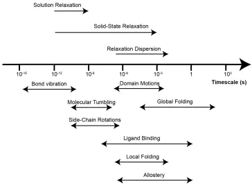
Figure 1.8.Examples of time scales of dynamic processes in proteins and relaxation measurements to obtain information on them.

In solid state NMR where molecules generally don’t tumble, relaxation measurements can be used to characterize time scales and amplitude of motion spanning from picoseconds – milliseconds. In this work three types of relaxation measurements were used; R1, R1ρ and R1ρ relaxation

dispersion.

To understand how these measurements relate to protein dynamics it is useful to first introduce the longitudinal (R1=1/T1) and transverse

(R2=1/T2) relaxation rates. Excited nuclear spins will return to equilibrium

through these relaxation processes. Longitudinal relaxation refers to the loss of z magnetization and transverse relaxation refers to the loss of coherence of xy magnetization. Generally, relaxation processes occur through anisotropic interactions; chemical shift anisotropy (CSA) and dipolar couplings (also quadrupolar interactions but they are not considered here). CSA results in local magnetic fields that depend on bond vector orientations relative to the static magnetic field. When a protein rotates relative to the B0 field and/or the bond vector rotates

(33)

Through space dipolar couplings between pairs of nuclear spins depend on both distance between the spins and orientation towards the B0 field

(see equation 1.4). The distance and the orientation may change with time and thus leads to local magnetic field oscillations , which just as the CSA stimulates nuclear relaxation. In solution NMR, information on protein motion can then indirectly be obtained from measuring R1 and R2

relaxation rates. In order to quantify the ps-ns dynamics of a protein in solution heteronuclear NOEs (Nuclear Overhauser Effects) are generally also measured. The heteronuclear NOEs occur due to dipolar interactions between 1_{H and a hetero atom (}15_{N or} 13_{C), and as mentioned above}

dipolar interactions stimulate nuclear relaxation due to protein motions at ps-ns timescales. Site specific measurements of these three parameters can give a full characterization of ps-ns motions in a protein in solution.46

In the solid state however, to extract information on dynamics from relaxation rates, coherent effects also need to be considered. The discussion below about effects of coherent contributions to R1, R2 and R1ρ

relaxation are based on a review by Lewandowski47_{. Spin diffusion is a}

coherent effect, originating from the incomplete averaging of a strong network of dipolar couplings, i.e. it is difficult to extract information on protein dynamics from relaxation measurements unless spin diffusion is properly suppressed. For site specific measurements of R1 relaxation

rates, which are measured by following the magnetization aligned with the static magnetic field as a function of relaxation delay, spin diffusion will cause magnetization transfer between different sites leading to average relaxation rates over several sites and no site specific information. Since spin diffusion is caused by anisotropic dipolar couplings it can be suppressed. In proteins the strongest dipolar couplings are caused by protons, so diluting the proton network is an efficient way of suppressing spin diffusion. Fast MAS will also suppress spin diffusion as it depends on the term ½(3cos2_θ _{– 1). Generally, a}

combination of diluting the proton network with deuterium and using fast MAS is used to measure site specific R1 relaxation rates in proteins.

(34)

very strong radio frequency pulses would have to be used, which could heat up the sample and damage the equipment. For 15_N _R

1 relaxation

measurements, which are studied in chapters 2 and 3, the variant of spin diffusion one needs to worry about is proton-driven spin diffusion (PDSD) and it is assisted by 1_H-15_{N dipolar couplings. It has been shown that}

even in fully protonated proteins PDSD is sufficiently suppressed to allow site specific 15_N _R

1 measurements already at 20 kHz MAS48–50. The

strength of the dipolar couplings depend on the gyromagnetic ratios of the coupled nuclei leading to that it is more difficult to suppress spin diffusion for 13_{C than for} 15_{N and even more difficult for} 1_{H. We}

investigate the use of 1_H _R

1 measurements with 100 kHz MAS, not to

measure dynamics, but to study protein – protein interfaces in chapter 2.

While R1 relaxation rates report on dynamics at picosecond – nanosecond

time scales R2 report on dynamics on nanoseconds – millisecond motions.

R2 relaxation is called spin – spin relaxation or transverse relaxation and

occur due to decay of magnetization in the xy-plane, perpendicular to the static magnetic field. An important challenge when measuring R2

relaxation rates is that coherent effects dominate the decay rates, in particular dipolar dephasing, which originates from strong 1_H-1_{H dipolar}

couplings. As mentioned earlier 1_H-1_{H dipolar couplings are the most}

difficult to suppress and even if fast MAS (> 60 kHz) and a high degree of deuteration (10% back-exchange of exchangeable protons) is applied it is very challenging to measure R2 relaxation rates in proteins. It is

though possible to measure R1ρ relaxation to get information on

nanosecond – millisecond motion. R1ρ relaxation rates are measured by

following the decay of magnetization under a spin-lock field. For 15_N _R

1ρ

measurement the coherent contributions can be sufficiently suppressed by a > 10 kHz spin-lock pulse and > 45 kHz MAS even in fully protonated proteins47_{. In chapter 3,} _R

1 and R1ρ relaxation are investigated and

related to protein motion for the protein GB1 in crystals and in a precipitated complex with IgG.

(35)

millisecond timescales and are measured by quantifying R2 or R1ρ

relaxation rates at varying lock frequencies. However as the lock field strength needs to be varied and one cannot rely on the spin-lock to help suppressing dipolar dephasing, higher levels of deuteration and/or faster MAS speed needs to be applied compared to standard R1ρ

relaxation measurements. Ma et al. showed that dipolar dephasing was sufficiently suppressed with 39.5 kHz MAS in a 50% back-exchanged perdeuterated crystalline sample of the small protein ubiquitin.51 _In

chapter 4 we show that we can access microsecond motion in the small protein GB1 in a > 300 kDa complex with full length human IgG.

1.4 NMR structure calculations

NMR, both in solution and in solid state, is a powerful tool for solving structures of biomolecules. Traditionally this is a very time consuming process but recent developments in NMR instrumentation and automation of structure calculation software have significantly shortened the time it takes from the first NMR experiments until a final structure can be determined. In order to determine a structure using NMR it is required to assign resonances relating to the atoms of the protein and to obtain distance restraints. In solution NMR the distance restraints are typically obtained from 2D and/or 3D NOESY (Nuclear Overhauser Effect SpectroscopY) experiments. This is often supplemented with torsion angle restraints, that for example can be calculated from the chemical shifts using the software TALOS+52_{. It is also possible to add restraints}

obtained from other types of NMR experiments and if there is information available from other sources that would aid the calculation it can also be added. There are several different software packages available for structure calculations as compared in the Critical Assessment of Automated Structure Determination of Proteins from NMR Data (CASD NMR)53_{, some of which use the traditional method described here and}

some of which calculate the structure based on chemical shifts.

(36)

13_C-13_{C distances rather than the} 1_H-1_{H distances commonly used in}

solution NMR. However with MAS speeds of 100 kHz and above it is now possible to use a similar approach as in solution NMR which has been demonstrated with fully protonated proteins54 _{and a combination of}

100% back exchanged perdeuterated protein for 1_HN_-1_HN _distance

restraints and partly labelled protein for distance restraints between methyl groups55_{. In the work presented here UNIO ATNOS-CANDID, with}

CYANA as molecular dynamics software was used for the structure calculation of teixobactin presented in chapter 5.

1.4.1 Resonance assignments in solution and solid state

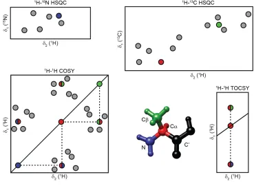
There are several different approaches to obtain full chemical shift assignments of proteins and peptides. For smaller peptides (up to around 20-30 residues), it might be sufficient to use 2D experiments with unlabelled material in solution. Figure 1.9 shows the approach for assignments using 2D spectra. The 1_H-1_{H COrrelation SpectroscopY}

(COSY) experiment gives a walk through each residue, where the cross -peaks that show up are coupled. The diagonal shows -peaks of the protons with itself. The example in the figure is alanine, where the first

diagonal peak from the top is Hβ-Hβ, following the dotted line leads to Hβ-Hα, horizontally to the diagonal is Hα-Hα, following the dotted line

vertically leads to Hα-HN _{and finally vertical to the diagonal shows H}N_-HN_.

The same information can be obtained from the 1_H-1_{H Total COrrelation}

SpectrosopY (TOCSY) experiment, but in a TOCSY all correlations between spins in a spin system is shown for each proton. This approach doesn’t give any interresidue information, which has to be obtained from interresidual HN_-HN _{peaks in} 1_H-1_{H NOESY spectra. If a peptide chain}

(37)

[image:37.595.134.503.75.345.2]

Figure 1.9.Schematic drawing of 2D assignment spectra used in solution NMR. Peaks resulting from alanine are highlighted in the figure.

If labelling is possible the assignment becomes easier, as 3D experiments can be recorded. Figure 1.10 shows an approach based on a combination of two 3D experiments. CBCANH gives the correlations between the NH

group of residue n and the Cα (positive peaks, red-yellow in fig1.10) and Cβ (negative peaks, green-blue in fig 1.10) from residues n and n-1,

while CACB(CO)NH only gives the peaks between an NH group of residue

n and the Cα and Cβ from residue n-1. With these two experiments a

backbone walk through the peptide chain to achieve assignments for all

N, HN_{, Cα and Cβ can be performed. It is often required, in larger}

systems or if the peptide chain contains many similar residues, to acquire additional spectra connecting the C’ to HN_{as the chemical shift dispersion}

of C’ is often larger than that of Cα. In this respect it should also be

mentioned that it is useful to assign atoms that are not directly needed for the structure calculation (e.g. C’) since chemical shifts also contain structural information in itself (which is discussed in chapter 5). If a 3D

hCCH TOCSY is acquired as well, the Hα, Hβ and side chain carbons and

(38)

[image:38.595.141.506.65.608.2]

Figure 1.10. Example strips from solution NMR 3D assignment spectra for [U-13C,15N]teixobactin in DPC micelles. Spectra acquired at 700 MHz1H Larmor frequency. DGN = D-Glutamine, DAI = D-allo-Isoleucine. The colour gradient from red to yellow represents the intensities of positive peaks. The colour gradient from green to blue represents the intensities of negative peaks.

In proton detected experiments in the solid state similar 3D experiments can be recorded. In figure 1.11 example strips of the assignment spectra for [U-13_C,15_{N]teixobacin in complex with natural abundance lipid II are}

(39)

transfers whereas the hCOCAHA uses dipolar recoupling enhanced by amplitude modulation (DREAM)56_{transfer between C’ and Cα. The}

[image:39.595.166.468.188.637.2]

DREAM also transfers to the Cβ from the C’ (however the spectrum was folded and therefore only Cα was considered in this case), and hence also gives the assignments for Cβ and Hβ.

Figure 1.11. Example strips from assignment spectra of [U-13C,15N]teixobactin in a sedimented complex with natural abundance lipid II in deuterated DPC micelles. Spectra acquired at 600 MHz1H Larmor frequency with 90 kHz MAS. DGN = D-glutamine, DAI = D-allo-isoleucine.

(40)

homonuclear dipolar couplings by fulfilling the double quantum HOmonucleaR ROtary Resonance (HORROR) condition:

= (1.9)

where ω1 is the nutation frequency of the adiabatic pulse in the DREAM

experiment. Another homonuclear recoupling technique called radio frequency driven recoupling (RFDR)57 _{is used to obtain} 1_{H –} 1_{H distance}

restraints, similar to NOESY in solution NMR. In an RFDR experiment a

train of rotor synchronized π pulses is applied on the 1_{H channel to}

recouple the homonuclear dipolar couplings, the longer the train of pulses is the further the magnetization is transferred.

1.4.2 CYANA libraries

When calculating a 3D structure based on NMR data it is necessary to use a molecular dynamics software. CYANA performs molecular dynamics calculations using torsion angle dynamics58_{. The degrees of freedom are}

based on the number of torsion angles, which are much smaller than the Carthesian coordinates and hence CYANA is much faster than molecular dynamics software that uses Carthesian space dynamics.

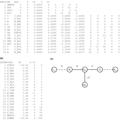
Many lipid II binders contain peptides with non-standard amino acid residues and in order to perform structure calculations on these kinds of molecules library entries for a molecular dynamics software need to be produced. In order to produce library entries for non-standard residues it is necessary to understand how CYANA libraries work. Torsion angles are defined in CYANA library files following a tree structure with a base rigid body that is fixed in space and n rigid bodies that are connected by n rotatable bonds. The rigid base is the amino acid backbone starting at the N-terminus, it then branches out and terminates at the end of the side-chains and C-terminus58_{. The CYANA library files are built as shown}

(41)

atom included in the residue (13), which means that atom number 14 belongs to the next residue in the chain. The peptide bonds are defined like this, so that each entry in the library representing a standard amino acid starts with C and O of the previous residue and ends with N of the following residue. The second line in the library entry defines the first

torsion angle, which for all standard amino acids is ω (OMEGA). Each

angle is defined by exactly 4 atoms and for side chain angles also a fifth atom is included which represents the last atom being affected by

changing the angle. For ω the 4 atoms defining it are Cn-1 (2), On-1 (1), Nn

(3) and Hn (4), since it is a backbone torsion angle the fifth number is 0.

Continuing down the library entry we see the other three torsion angles

of alanine φ (PHI), χ1(CHI1) and ψ (PSI), where χ1 is the only side chain

(42)

[image:42.595.113.522.82.497.2]

Figure 1.12.Structure of CYANA library entry58. (a) example of library entry for the amino acid alanine. (b) Definition of atom types used in Cyana. (c) Tree structure of alanine.

(43)

The standard CYANA library includes all standard amino acid residues, RNA bases and DNA bases but if structure calculations with non-standard residues are to be performed, library entries for these have to be

produced. Recently a software called Cylib59 _{was released. Cylib can}

convert any molecular topology description from the PDB Chemical Component Dictionary (CCD) into CYANA library entries. This makes it much easier to perform structure calculations of peptides containing non-standard residues as it is tedious process to produce library entries

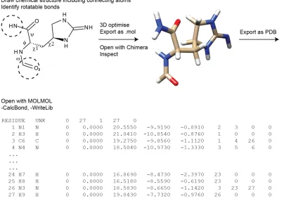
manually. There are however cases where Cylib doesn’t work; (i) if there is no entry in the PDB CCD or (ii) if the connection between residues is not a standard peptide bond. In these cases an entry has to be created manually. Figure 1.13 shows the steps needed to prepare a new library entry. Here L-allo-enduracidine was used as example, which is an unusual amino acid present in teixobactin. The first step is to obtain starting coordinates and connections for all the atoms in the new residue. This can be done by drawing it in any molecule drawing software and convert it into a 3D drawing. Then it needs to be saved in a format that UCSF Chimera60 _{can read, for example as a mol file. If there is an}

available 3D structure of the residue or a similar residue this first step can be skipped and one can download the 3D structure and add the overlapping atoms to the connecting residues (in dotted circles at the top of Figure 2), which can be done in UCSF Chimera. The file should then be saved as a PDB file, which can be read by MOLMOL61 _{and a file containing}

(44)

[image:44.595.112.516.76.362.2]

Figure 1.13. Stepwise explanation for how to create Cyana library entries for non-standard amino acids. Here with L-allo-enduracidine as example.

1.4.3 Structure calculations using UNIO-ATNOS CANDID

(45)

dependent and the intensity of the cross-peaks in NOESY spectra will be proportional to the distance between two protons.

To obtain distance restraints from NOE spectra in solution NMR the chemical shifts of the two protons involved in the cross peak needs to be unambiguously assigned. As the chemical shift range of protons in proteins is fairly small < 15 ppm and the accuracy of which NOE cross peaks can be measured is limited it is very difficult to unambiguously assign the peaks. By using 3D HSQC-NOESY spectra, which are resolved through an additional 13_{C or} 15_{N chemical shift, it becomes easier than for}

2D 1_{H –} 1_{H NOESY experiments but is still very challenging. NOESY}

spectra can also be quite noisy and contain artefacts making the process even more challenging. Traditionally picking and assigning NOE cross peaks was an iterative process where a preliminary 3D structure was calculated from a limited amount of unambiguously assigned peaks. The preliminary 3D structure was then used to identify more peaks. Luckily, due to a lot of effort into software development it is now much easier and faster to perform NMR structure calculations. There are several software packages that can achieve high quality 3D structures of proteins with unassigned peak lists from NOESY spectra compared in the CASD-NMR53_.

Of the software packages tested in that study only two submitted results based on raw spectra as input, UNIO and Ponderosa. Using raw spectra as input is very appealing as it eliminates time consuming and error prone peak picking. As previously mentioned UNIO ATNOS-CANDID was used for the structure calculation of teixobactin presented chapter 5.

UNIO includes different algorithms for backbone assignments (MATCH)62_,

side-chain assignments (ATNOS-ASCAN)63,64 _{and NOE assignments and}

structure calculations (ATNOS-CANDID)63,65_{. In a structure calculation}

(46)

and transforms them into distance restraints for CYANA and a preliminary structure is calculated. This structure is then used by ATNOS to identify more peaks and by CANDID to assign them and add more distance restraints for the next structure calculation, the structure based criteria for peak validation in ATNOS is loosened up, while the acceptance for NOE assignment and distance restraints by CANDID is tightened. Generally 7 cycles are performed in a standard structure calculation using UNIO ATNOS-CANDID.

Two important elements that were incorporated in CANDID are network anchoring and constraint-combination. In network anchoring the assignment for each NOE cross-peak is weighted by how well it fits in a network including all other NOE assignments. This works because any network of correct NOE cross-peak assignments can be seen as a self-consistent set. Constraint combination is used to combine several distance restraints into one in order to reduce the risk of artefacts influencing the structure calculation. This is especially important for long-distance restraints that have a larger impact on the structure calculation.65

The same procedure works in solid state NMR, but RFDR spectra are normally used instead of NOESY. There are however not yet any published structures calculated from solid state NMR data where raw spectra have been used as input. A few structures have recently been published using the “solution NMR” approach in UNIO with unassigned peak lists from spectra of fully protonated proteins in solid state NMR54_.

1.5 References

(1) Gronenborn, A.; Filpula, D.; Essig, N.; Achari, A.; Whitlow, M.; Wingfield, P.; Clore, G. Science (80-. ). 1991,253 (5020), 657.

(2) Frericks Schmidt, H. L.; Sperling, L. J.; Gao, Y. G.; Wylie, B. J.; Boettcher, J. M.; Wilson, S. R.; Rienstra, C. M. J. Phys. Chem. B

2007, 111 (51), 14362.