Abstract—In this paper, we propose a novel Takagi-Sugeno- Kang type interval-valued neural fuzzy system with asymmetric fuzzy membership functions (called TIVNFS-A). In addition, the corresponding type reduction procedure is integrated in the adaptive network layers to reduce the amount of computation in the system. Based on the Lyapunov stability theorem, the TIVNFS-A system is trained by the back-propagation (BP) algorithm having an optimal learning rate (adaptive learning rate) to guarantee the stability and faster convergence. Finally, the TIVNFS-A with the optimal BP algorithm is applied in nonlinear system identification to demonstrate the effectiveness and performance.
Index Terms—interval-valued fuzzy system, Lyapunov stability theorem, asymmetric membership function, TSK type, nonlinear system
I. INTRODUCTION
n recent years, fuzzy neural networks (FNNs) are used successfully in many applications [5, 7-9, 10, 13-21, 25, 27-28], such as classifications, prediction, nonlinear system and control. FNNs are combined the advantages of fuzzy system and neural network. Recently, interval type-2 fuzzy logic systems (T2FLSs) have got lots of attention in many applications due to their ability to model uncertainties. Besides, many literatures have shown that an interval T2FLS is the same as an interval-valued fuzzy logic system (IVFLS) [1-2, 23, 26]. IVFLSs are more complex than type-1 fuzzy logic systems (T1FLSs). IVFLSs have better performance than T1FLSs on the applications of function approximation, system modeling and control. Combining the advantages of IVFLSs and neural network, interval-valued fuzzy neural network (IVFNN) systems are presented to handle the system uncertainty [6, 16, 18].
By designing the fuzzy partition and rule engine, symmetric and fixed membership functions (MFs), like Gaussian or triangular, are usually used to simplify the design procedure. Accordingly, a large number of rules should be used to accomplish the explicit approximation accuracy [5, 15, 17]. In order to solve these problems, the asymmetric fuzzy MFs (AFMFs) have been adopted [3, 11, 17-20, 24]. These results demonstrated that using AFMFs can improve
This work was supported in part by the National Science Council, Taiwan, R.O.C., under contracts NSC-97-2221-E-155-033-MY3.
Ching-Hung Lee is with Department of Electrical Engineering, Yuan-Ze University, Chung-li, Taoyuan 320, Taiwan. (phone: +886-3-4638800, ext: 7119; fax: +886-3-4639355, e-mail: [email protected]).
the modeling capability. The asymmetric fuzzy MFs provide the ability of high flexibility and more accurate [18]. In addition, the Takagi-Sugeno-Kang (TSK) type FLSs have the universal approximation capability [4]. By the combination of these above advantages, the TSK-type interval-valued neural fuzzy system with asymmetric membership functions (TIVNFS-A) is proposed in this paper. In addition, the corresponding type reduction procedure is integrated in the adaptive network layers to reduce the amount of computation in the system. Therefore, the Karnik-Mendel type-reduction procedure is removed.
For training and designing the neural fuzzy systems, the back-propagation algorithm is widely used and a powerful training technique [5, 8, 25]. For each training cycle, all parameters of neural fuzzy system are adjusted to reduce the error between the desired and actual output. Herein, based on the Lyapunov stability theorem, the TIVNFS-A system is trained by the back-propagation (BP) algorithm having an optimal learning rate (adaptive learning rate) to guarantee the stability and faster convergence.
The rest of this paper is as follows. Section II introduces the construction of AFMFs and TIVNFSF-A. The back- propagation algorithm with the optimal learning rate is introduced in Section III. Section IV shows the simulation results of nonlinear system identification using TIVNFS-A with optimal BP algorithm. Finally, the conclusion is given.
II. TAKAGI-SUGENO-KANG-TYPE INTERVAL-VALUED NEURAL FUZZY
SYSTEMS
In this paper, we propose a TSK-type interval-valued neural fuzzy system with asymmetric membership functions (TIVNFS-A), which is a modification of type-2 fuzzy neural networks (or interval-valued neural fuzzy systems). We adopted interval-valued asymmetric MFs and the TSK-type consequent part to develop the TIVNFS-A. We first introduce the network structure of TIVNFS-A. In general, given the system input data xi, i=1 ,2,L ,n, and the TIVNFS-A’s output yˆ, the jth fuzzy rule can be expressed as:
Rule j: IF x1 is F1j
~ and … and x n is Fnj
~ , THEN Yj=Cj0+Cj1x1+Cj2x2+…+ Cjnxn, (1) where j=1, 2, …, M; Cj0 and Cji are the consequent fuzzy sets, Yj is the output of the jth rule (a linear combination operation), and Fij
~ is the antecedent fuzzy set. The fuzzy MFs of the antecedent part Fij
~ are the asymmetric interval-valued fuzzy
Stable Learning Mechanism for Novel
Takagi-Sugeno-Kang Type Interval-valued
Fuzzy Systems
Yi-Han Lee and Ching-Hung Lee, Member IAENG
sets (IVFSs) that are shown in Fig. 1, which are different from typical Gaussian MFs. Several approaches indicate that using asymmetric MFs can improve approximation accuracy [3, 12, 18, 19-21, 25]. The asymmetric IVFSs are generated from four Gaussian functions, as shown in Fig. 1. The construction of asymmetric IVFSs was introduced in literature [18]. Subsequently, the fuzzy sets of the consequent part Cj0 and Cji are designed to be convex, normal type-1 fuzzy subsets. A TIVNFS-A with M fuzzy rules is implemented as the six-layer network shown in Fig. 2. The signal propagation and the operation functions of the nodes are indicated in each layer. In the following description, (k)
i
O denotes the ith output of a node in the kth layer.
[image:2.595.49.280.282.533.2]asymmetric IVFS
Figure 1: Constructed asymmetric interval valued fuzzy set (IVFS) [18].
Layer 2: Membership layer Layer 5: TSK layer
Layer 1: Input layer Layer 3: Rule layer Layer 4: Left-most &
Right-most layer Layer 6: Output layer
1
x xi xn
11
~
F F~1j F~1M F~i1 F~ij F~iM F~n1 F~nj F~nM
∏
∏ ∏∏ ∏∏
Σ
Σ Σ Σ Σ Σ Σ
] [1 1
l lω
ω [11]
r rω
ω
] [ l
j l jω
ω
] [ l
M l Mω
ω
] [ r
j r jω
ω
] [ r
M r Mω
ω
] [fMfM
]
[f1f1 [fjfj]
Σ Σ
l
T1
l j
T l M
T Tr
1 Trj
r M
T
y
ˆ
Layer 2: Membership layer Layer 5: TSK layer
Layer 1: Input layer Layer 3: Rule layer Layer 4: Left-most &
Right-most layer Layer 6: Output layer
1
x xi xn
11
~
F F~1j F~1M F~i1 F~ij F~iM F~n1 F~nj F~nM
∏ ∏
∏ ∏∏∏ ∏∏∏
Σ
Σ Σ Σ Σ Σ Σ
] [1 1
l lω
ω [11]
r rω
ω
] [ l
j l jω
ω
] [ l
M l Mω
ω
] [ r
j r jω
ω
] [ r
M r Mω
ω
] [fMfM
]
[f1f1 [fjfj]
Σ Σ
l
T1
l j
T l M
T Tr
1 Trj
r M
T
y
[image:2.595.307.550.480.602.2]ˆ
Figure 2: Diagram of the proposed TIVNFS-A with M rules.
Layer 1 (Input Layer): For the ith node of layer 1, the net input and the net output are written as
i i x
O(1)=
(2) where i=1, 2, …, n, xi represents the ith input to the ith node of layer 1. The nodes in this layer only transmit input values to the next layer directly.
Layer 2 (Membership Layer): In this layer, each node performs an asymmetric IVFS Fij
~
, as shown in Fig. 1, i.e.,
T i F i F T ij ij i F
ij O O O O O
O
ij ij
ij( ) [ ] [ ( ) ( )]
) 1 ( ~ ) 1 ( ~ ) 2 ( ) 2 ( ) 1 ( ~ ) 2
( =μ = = μ μ (3)
where the subscript “ij” indicates the jth term of the ith input, where j=1, …, M.
Layer 3 (Rule Layer): The links in this layer are used to implement antecedent matching. We choose the product t-norm because it is easy to implement in a neural network. Thus, the firing strength associated with the jth rule is the following:
) ( )
( (1)
~ )
1 ( 1 ~
1 F n
F
j O O
f
nj j
μ
μ ∗ ∗
= L (4)
) ( )
( (1)
~ )
1 ( 1 ~
1 F n
F
j O O
f
nj
j μ
μ ∗ ∗
= L (5) where ~(⋅)
ij
F
μ and ~(⋅)
ij
F
μ are the lower and upper membership grades of ~(⋅)
F
μ , respectively. Therefore, a simple product operation is used. Then,
[
]
.1 ) 2 (
1 ) 2 ( )
3 ( ) 3 ( ) 3 (
T n i
ij n
i ij T
j j
j O O O O
O
⎥⎦ ⎤ ⎢⎣
⎡ =
=
∏
∏
= =
(6)
Layer 4 (Left-most and right-most layers): The weighting vectors of TIVNFS-A are interval-valued
[
l]
Tj l j ω
ω and
[
r]
T j r j ωω , where l
j l
j ω
ω < and r.
j r j ω
ω < The following vector notations are used for clarity:
T l M l l
] [ω1 ω
ω = L ,
[
1]
,T l M l
l ω ω
ω = L r T
M r r
] [ω1 ω
ω = L ,
and
[
r]
TM r
r ω ω
ω = 1 L . Therefore, the output for layer 4 is
]
[
r Tj r j
j r j j r j l
j l j
j l j j l j T jr jl j
O O
O O
O O O
⎥ ⎥ ⎦ ⎤ + + ⎢
⎢ ⎣ ⎡
+ + =
=
ω ω
ω ω
ω ω
ω
ω (3) (3) (3) (3) )
4 ( ) 4 ( ) 4
( (7)
This expression calculates the left-most points, (4)
jl
O , and right-most points, (4).
jr
O According to previously reported results [6], the type reduction is integrated into the adaptive network layers. Therefore, the Karnik-Mendel type-reduction procedure is removed. Because the iterative procedure for finding coefficients R and L is not necessary, the computational effort can be reduced effectively.
Layer 5 (TSK Layer): Because the asymmetric IVFSs are used for the antecedents and because the interval sets are used for the consequent sets of the TSK rules, it is possible to state that the Cji terms are interval sets. In other words, Cji=[cji-sji cji+ sji]T, where i=1,…, n, and j=1,…, M. In this expression, cji denotes the center (mean) of Cji, and sji denotes the spread of Cji, i=1, 2, …, n and j=1, 2, …, M. Therefore, the consequent part of Rule j is
T n
i i ji j
n i
i ji j
n i
i ji j
n i
i ji j
j
x s s x c c
x s s x c c T
] ) (
) (
) (
) [(
1 0 1
0
1 0 1
0
∑
∑
∑
∑
= =
= =
+ + +
+ − +
=
(8)
where sji≥0. The output of layer 5 is
[
]
.1 ) 4 ( 1
) 4 (
1 ) 4 ( 1
) 4 (
) 5 ( ) 5 ( ) 5 (
T M j
jr M j
r j jr M
j jl M j
l j jl T
r l
O T O O
T O O
O O
⎥ ⎥ ⎥ ⎥
⎦ ⎤
⎢ ⎢ ⎢ ⎢
⎣ ⎡ = =
∑
∑
∑
∑
= =
= =
(9)
Layer 6 (Output Layer): Layer 6 is the output layer, which is used to implement the defuzzification operation. The output is the following:
. 2
) 5 ( ) 5 ( ) 6
( Ol Or
O = + (10) As the above introduction, the interval-valued fuzzy sets are used to design the antecedents and interval type-1 fuzzy sets are used to design the consequent sets of an interval-valued TSK rule. Directing our attention to (9), we can see that (4)
j
O and Tj are interval type-1 fuzzy sets. Hence,
) 5 (
TSK
O is an interval type-1 fuzzy set. We only need to compute its two end-points (5)
l
O and (5)
r
O to compute (5)
TSK
right-most points. Without operating the iterative procedure of KM algorithm described in [12] for finding coefficients R and L . Therefore, the TIVNFS-A can reduce the computational complexity successfully.
III. LEARNING OF TIVNFS-ASYSTEMS
In this paper, we adjust the parameter of TIVNFS-A by the back-propagation (BP) algorithm to enhance performance [5, 8, 15, 25]. The back-propagation algorithm is based on the gradient descent method to fine the optimal solution of each parameter.
A. Back-propagation Algorithm
For clarification, we consider the signal-output system and define the error cost function
2
) ( 2 1 ) (k e k
E = , (11) where e(k) y (k) yˆ(k) y (k) O(6)(k),
d d − = −
= that yˆ(k) and
) (k
yd are the TIVNFS-A’s output and desired output for
discrete time k, respectively. Using the gradient descent method, the parameters updated law of the parameters is
, ) ( )
( ) 1
( ⎟
⎠ ⎞ ⎜
⎝ ⎛
∂ ∂ − + = +
W W
Wk k η E k (12) where η is the learning rate. W=
[
W ,W ,γ ,Wω ,C]
T are theadjustable parameters, where C is the parameters of TSK layer, Wω is the consequent weights, W is the parameters
of lower MFs, W is upper MFs parameters, and γ is the column vectors, i.e.,
[
]
[
]
[
]
[
]
., , ,
T r l r l
T r l r l
T r l r l
T
m m
m m
s c
σ σ
σ σ
ω ω ω ω
ω
= = = =
W W W C
(13)
Considering ∂E(k) ∂W, we have
, ) ( ˆ ) ( ) ( ˆ ) ( ˆ
) ( ) (
) ( ) (
W W
W ∂
∂ − = ∂ ∂ ∂ ∂ ∂ ∂ = ∂
∂ y k ek yk
k y
k e k e
k E k
E (14)
thus,
, ) ( ) ( ) (
) ( ˆ ) ( ) ( ) 1 (
) 6 (
W W
W W
W
∂ ∂ ⋅ ⋅ + =
∂ ∂ ⋅ ⋅ + = +
k O k e k
k y k e k k
η η
(15)
where e(k)=yd(k)−yˆ(k). The remaining work involves finding the corresponding partial derivative with respect to each parameter. For the BP algorithm, the remaining works are the derivations of gradient for parameters W ,W ,γ ,Wω,
and C. The derivations are omitted due to the writing space. Similar details can be found in literature [18].
B. Optimal Learning Rate
The learning rate plays an important role in BP algorithm. A small value of learning rate leads the speed of convergence will be slower. The large value of learning rate leads the
speed of convergence is faster but it might produce local minimum. Hence, the selection of the learning rate is importantly but it is not easy to choosing suitably. Thus, we use the Lyapunove function to find the optimal learning rate [5, 15, 29]. At first, we defined the positive Lyapunov candidate
) ( 2 1 ) ( )
(k E k e2 k
V = = . (16) In general, e(k+1)−e(k)=Δe(k). Thus, we have
[
]
(
)
[
]
[
( ) 2 ( ) ( )]
,2 1
) ( ) ( 2 ) ( 2 1
)) ( ) 1 ( ( )) ( ) 1 ( ( 2 1
) ( ) 1 ( ) (
2 k ek e k
e
k e k e k e
k e k e k e k e
k V k V k V
Δ ⋅ + Δ =
Δ + ⋅
Δ =
+ + ⋅ − + =
− + = Δ
(17)
where Δe(k)≈(∂e∂W)ΔW ,thus, according to the parameter update rule of BP algorithm, ΔW=−η(∂E ∂W). And we can obtain
⎟ ⎠ ⎞ ⎜ ⎝ ⎛ ∂
∂ ⋅ ⋅ − = ⎟ ⎠ ⎞ ⎜
⎝ ⎛
∂ ∂ − ∂
∂ ≈ Δ
W W
W
y k e E
e k
e( ) η η ( ) ˆ . (18)
Thus,
. ˆ 2
ˆ 2
1
ˆ ˆ
2 2 1 ) (
2 2
2
4 2
2 2 2
⎥ ⎥ ⎦ ⎤ ⎢
⎢ ⎣ ⎡
⎟ ⎠ ⎞ ⎜ ⎝ ⎛ ∂
∂ ⋅ − ⎟ ⎠ ⎞ ⎜ ⎝ ⎛ ∂
∂ ⋅ ⋅ − =
⎥ ⎥ ⎦ ⎤ ⎢
⎢ ⎣ ⎡
⎟ ⎠ ⎞ ⎜ ⎝ ⎛ ∂
∂ ⋅ ⋅ + ⎟ ⎠ ⎞ ⎜ ⎝ ⎛ ∂
∂ ⋅ ⋅ − = Δ
W W
W W
y y
e
y e y
e k
V
η η
η η
(19)
Next, according to the Lyapunov stability theory, we should choose a proper value of η such that ΔV(k)≤0. Therefore, we can obtain the stability condition for learning rate
2 ˆ 0
2
< ⎟ ⎠ ⎞ ⎜ ⎝ ⎛ ∂
∂ <
W
y
η . (20)
Define
2
ˆ ⎟ ⎠ ⎞ ⎜ ⎝ ⎛ ∂
∂ ⋅ =
W
y η
λ and rewrite (19) as
(
2)
0. )( )
( = ⋅ ⋅ − + ≤
ΔV k V k λ λ (21) Then we have
(
2)
0 )( ) ( ) 1
(k+ −V k =V k ⋅λ⋅ − +λ ≤
V (22)
and
(
1 2)
0. )( ) 1
(k+ =V k ⋅ − λ+λ2 ≤
V (23)
Thus, the optimal learning rate η can be obtained
2
* ˆ
−
⎟ ⎠ ⎞ ⎜ ⎝ ⎛ ∂
∂ =
W
y
η (24) such that λ=1. Note that W∈ℜD, where D is the dimension of the problem. Therefore, the choice of optimal learning rate guaranteed the faster convergence is
2
* 1 ˆ
−
⎟ ⎠ ⎞ ⎜ ⎝ ⎛ ∂
∂ =
W
y D
- Optimal learning of C , 2 1 1 ) ( ˆ 1 -2 1 ) 4 ( ) 4 ( 1 ) 4 ( ) 4 ( 2 0 0 ⎥ ⎥ ⎥ ⎥ ⎦ ⎤ ⎢ ⎢ ⎢ ⎢ ⎣ ⎡ ⎟ ⎟ ⎟ ⎟ ⎠ ⎞ ⎜ ⎜ ⎜ ⎜ ⎝ ⎛ + = ⎟ ⎟ ⎠ ⎞ ⎜ ⎜ ⎝ ⎛ ∂ ∂ =
∑
∑
= = − M j jr jr M j jl jl j c O O O O D c k y D jη (26)
, 2 1 ) ( ˆ 1 -2 1 ) 4 ( ) 4 ( 1 ) 4 ( ) 4 ( 2 ⎥ ⎥ ⎥ ⎥ ⎦ ⎤ ⎢ ⎢ ⎢ ⎢ ⎣ ⎡ ⎟ ⎟ ⎟ ⎟ ⎠ ⎞ ⎜ ⎜ ⎜ ⎜ ⎝ ⎛ + ⋅ = ⎟ ⎟ ⎠ ⎞ ⎜ ⎜ ⎝ ⎛ ∂ ∂ =
∑
∑
= = − M j jr jr M j jl jl i ji c O O O O x D c k y D jiη (27)
, 2 1 1 ) ( ˆ 1 -2 1 ) 4 ( ) 4 ( 1 ) 4 ( ) 4 ( 2 0 0 ⎥ ⎥ ⎥ ⎥ ⎦ ⎤ ⎢ ⎢ ⎢ ⎢ ⎣ ⎡ ⎟ ⎟ ⎟ ⎟ ⎠ ⎞ ⎜ ⎜ ⎜ ⎜ ⎝ ⎛ + − = ⎟ ⎟ ⎠ ⎞ ⎜ ⎜ ⎝ ⎛ ∂ ∂ =
∑
∑
= = − M j jr jr M j jl jl j s O O O O D s k y D jη (28)
. 2 1 ) ( ˆ 1 -2 1 ) 4 ( ) 4 ( 1 ) 4 ( ) 4 ( 2 ⎥ ⎥ ⎥ ⎥ ⎦ ⎤ ⎢ ⎢ ⎢ ⎢ ⎣ ⎡ ⎟ ⎟ ⎟ ⎟ ⎠ ⎞ ⎜ ⎜ ⎜ ⎜ ⎝ ⎛ + ⋅ = ⎟ ⎟ ⎠ ⎞ ⎜ ⎜ ⎝ ⎛ ∂ ∂ =
∑
∑
= = − M j jr jr M j jl jl i ji s O O O O x D s k y D jiη (29)
- Optimal learning of Wω
, 2 1 1 ) ( ˆ 1 -2 ) 4 ( ) 3 ( 1 ) 4 ( ) 5 ( 2 ⎥ ⎥ ⎥ ⎥ ⎦ ⎤ ⎢ ⎢ ⎢ ⎢ ⎣ ⎡ ⎟ ⎟ ⎟ ⎟ ⎠ ⎞ ⎜ ⎜ ⎜ ⎜ ⎝ ⎛ + − ⋅ − = ⎟ ⎟ ⎠ ⎞ ⎜ ⎜ ⎝ ⎛ ∂ ∂ =
∑
= − l j l j jl j M j jl l l j l j O O O O T D k y D lj ω ω ω
ηω (30)
, 2 1 1 ) ( ˆ 1 -2 ) 4 ( ) 3 ( 1 ) 4 ( ) 5 ( 2 ⎥ ⎥ ⎥ ⎥ ⎦ ⎤ ⎢ ⎢ ⎢ ⎢ ⎣ ⎡ ⎟ ⎟ ⎟ ⎟ ⎠ ⎞ ⎜ ⎜ ⎜ ⎜ ⎝ ⎛ + − ⋅ − = ⎟ ⎟ ⎠ ⎞ ⎜ ⎜ ⎝ ⎛ ∂ ∂ =
∑
= − r j r j jr j M j jr r r j r j O O O O T D k y D rj ω ω ω
ηω (31)
, 2 1 1 ) ( ˆ 1 -2 ) 4 ( ) 3 ( 1 ) 4 ( ) 5 ( 2 ⎥ ⎥ ⎥ ⎥ ⎦ ⎤ ⎢ ⎢ ⎢ ⎢ ⎣ ⎡ ⎟ ⎟ ⎟ ⎟ ⎠ ⎞ ⎜ ⎜ ⎜ ⎜ ⎝ ⎛ + − ⋅ − = ⎟ ⎟ ⎠ ⎞ ⎜ ⎜ ⎝ ⎛ ∂ ∂ =
∑
= − l j l j jl j M j jl l l j l j O O O O T D k y D lj ω ω ω
ηω (32)
. 2 1 1 ) ( ˆ 1 -2 ) 4 ( ) 3 ( 1 ) 4 ( ) 5 ( 2 ⎥ ⎥ ⎥ ⎥ ⎦ ⎤ ⎢ ⎢ ⎢ ⎢ ⎣ ⎡ ⎟ ⎟ ⎟ ⎟ ⎠ ⎞ ⎜ ⎜ ⎜ ⎜ ⎝ ⎛ + − ⋅ − = ⎟ ⎟ ⎠ ⎞ ⎜ ⎜ ⎝ ⎛ ∂ ∂ =
∑
= − r j r j jr j M j jr r r j r j O O O O T D k y D rj ω ω ω
ηω (33)
-Optimal learning of W
. 4 1 ) ( ˆ 1 2 2 ) 3 ( 1 ) 4 ( ) 5 ( ) 3 ( 1 ) 4 ( ) 5 ( 2 − = = − ⎥ ⎥ ⎥ ⎥ ⎦ ⎤ ⎟⎟ ⎠ ⎞ ⎜⎜ ⎝ ⎛ − ∂ ∂ ⋅ ⎟ ⎟ ⎟ ⎟ ⎠ ⎞ + ⋅ ⋅ − + ⎢ ⎢ ⎢ ⎢ ⎣ ⎡ ⎜ ⎜ ⎜ ⎜ ⎝ ⎛ + ⋅ ⋅ − − = ⎟⎟ ⎠ ⎞ ⎜⎜ ⎝ ⎛ ∂ ∂ =
∑
∑
σ ω ω ω ω ω ω γ η m x O O O T O O O T k y D r j r j j r j M j jr r r j l j l j j l j M j jl l l j W W W (34)- Optimal learning of W
. 4 1 ) ( ˆ 1 2 2 ) 3 ( 1 ) 4 ( ) 5 ( ) 3 ( 1 ) 4 ( ) 5 ( 2 − = = − ⎥ ⎥ ⎥ ⎥ ⎦ ⎤ ⎟⎟ ⎠ ⎞ ⎜⎜ ⎝ ⎛ − ∂ ∂ ⋅ ⎟ ⎟ ⎟ ⎟ ⎠ ⎞ + ⋅ ⋅ − + ⎢ ⎢ ⎢ ⎢ ⎣ ⎡ ⎜ ⎜ ⎜ ⎜ ⎝ ⎛ + ⋅ ⋅ − − = ⎟ ⎠ ⎞ ⎜ ⎝ ⎛ ∂ ∂ =
∑
∑
σ ω ω ω ω ω ω γ η m x O O O T O O O T k y D r j r j j r j M j jr r r j l j l j j l j M j jl l l j W W W (35)- Optimal learning of γ
[image:4.595.51.547.52.773.2]. 2 1 1 ) ( ˆ 1 2 ) 3 ( 1 ) 4 ( ) 5 ( 1 ) 4 ( ) 5 ( 2 − = = − ⎥ ⎥ ⎥ ⎥ ⎦ ⎤ ⋅ ⎟ ⎟ ⎟ ⎟ ⎠ ⎞ + ⋅ − + ⎢ ⎢ ⎢ ⎢ ⎣ ⎡ ⎜ ⎜ ⎜ ⎜ ⎝ ⎛ + ⋅ − = ⎟ ⎟ ⎠ ⎞ ⎜ ⎜ ⎝ ⎛ ∂ ∂ =
∑
∑
ij j r j r j r j M j jr r r j l j l j l j M j jl l l j ij O O O T O O T D k y D ij γ ω ω ω ω ω ω γ ηγ (36)Fig. 3. Series-parallel model with the TIVNFS-A for nonlinear systems identification.
IV. SIMULATION RESULTS
In this section, the example for nonlinear system identification is presented to show the performance of the TIVNFS-A. All simulations were done by MATLAB in Intel(R) CORE 2 QUAD computer with clock rate of 2.4GHz and 3GB of main memory.
Consider the following nonlinear system
(
( ), ( 1), ( 2), ( ), ( 1))
) 1
(k+ = f y k y k− y k− uk u k−
yp p p p , (37)
where
(
)
. 1 ) 1 ( , , , , 2 3 2 2 4 3 5 3 2 1 5 4 3 2 1 x x x x x x x x x x x x x f + + + − =u and yp are system’s input and output. Herein, the series- parallel training scheme is adopted, as shown in Fig. 3. The approximated error is defined as follows
), ( ˆ ) ( )
(k y k yk
e ≡ p − (38)
where yˆ(k) denotes the TIVNFS-A’s output. Clearly, due to the static structure of TIVNFS-A, the input number should be set as 5. The training input is
) 10 sin( 6 . 0 ) 32 sin( 1 . 0 ) 25 sin( 3 . 0 )
(k k k k
u = π + π + π , (39)
⎪ ⎪ ⎪ ⎪
⎩ ⎪ ⎪ ⎪ ⎪
⎨ ⎧
< ≤ +
+
< ≤ −
< ≤
< <
=
. 1000 50
7 )
10 sin( 6 . 0
) 32 sin( 1 . 0 ) 25 sin( 3 . 0
, 750 00
5 0
. 1
, 500 50
2 0
. 1
, 250 0
) 25 sin(
) (
k k
k
k k
k k k
k u
π π π
π
(40)
The following RMSE is adopted to be the performance index
2 / 1
2( )/ )
( :
∑
k
N k e
RMSE , (41) where N is the number of training pattern.
The parameters of TIVNFS-A are l, l , r, r , l , l , m
m m
m σ σ
s c
r
r ,σ ,γ ,ω ,ω , ,
σ that are chosen randomly between [-1, 1]. The numbers of the TIVNFS-A’s rule is set to be 2, then the structure of TIVNFS-A is 2-4-2-4-2-1, and the numbers of parameter of TIVNFS-A is 56.
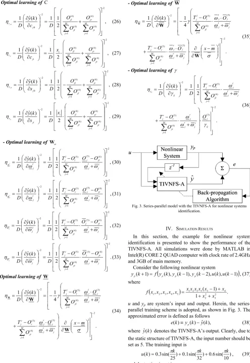
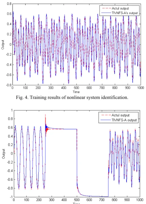
[image:5.595.314.539.53.232.2]Figures 4 and 5 show the results of nonlinear system identification after 50 epochs training and testing, respectively (solid line: actual output; dashed line: TIVNFS-A’s output). The convergence of RMSE is shown in Fig. 6.
Fig. 4. Training results of nonlinear system identification.
Fig. 5. Testing results of nonlinear system identification.
Fig. 6. The values of RMSE after training.
Illustration Comparison of the Optimal Learning Rate: Figure 7 and TABLE I show the comparison results between the TIVNFS-A system using the optimal learning rate η* and
fixed learning rate η. Obviously, we obtain the performance of BP algorithm with optimal learning rate is better than without optimal learning rate. The average RMSE of BP algorithm with η* was 0.002377 and The average RMSE of
[image:5.595.50.290.348.681.2]BP algorithm with optimal learning rate was 0.003203. Thus, the performance is more stable with optimal learning from the best and the worst value of RMSE.
Fig. 7. The values of RMSE of BP algorithm with optimal learning rate and without optimal learning rate.
TABLEI
THE COMPARISON RESULTS IN 10TIMES OF DIFFERENT LEARNING RATE
BP algorithm with optimal learning rate
BP algorithm with fixed learning rate
Best 0.001671 0.001696
Average 0.002377 0.003203
Worst 0.003458 0.006690
Times(sec) 21.904 15.808
Illustration Comparison of TIVNFS-A system: In this
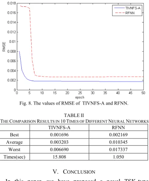
[image:5.595.313.542.382.545.2] [image:5.595.304.550.589.669.2]better than by RFNN. We solve the nonlinear system identification by TIVNFS-A successfully and the simulation result the better performance.
Fig. 8. The values of RMSE of TIVNFS-A and RFNN.
TABLEII
THE COMPARISON RESULTS IN 10TIMES OF DIFFERENT NEURAL NETWORKS
TIVNFS-A RFNN
Best 0.001696 0.002169
Average 0.003203 0.010345
Worst 0.006690 0.017337
Times(sec) 15.808 1.050
V. CONCLUSION
In this paper, we have proposed a novel TSK-type interval-valued neural fuzzy system with asymmetric fuzzy membership functions (TIVNFS-A) for application of nonlinear system identification. In addition, the corresponding type reduction procedure is integrated in the adaptive network layers to reduce the amount of computation in the system. Based on the Lyapunov stability theorem, the TIVNFS-A system is trained by the back-propagation (BP) algorithm having an optimal learning rate (adaptive learning rate) to guarantee the stability and faster convergence. Illustration examples are shown to demonstrate the effectiveness and performance of the proposed TIVNFS-A with optimal BP learning algorithm.
REFERENCES
[1] H. Bustince, “Indicator of Inclusion Grade for Interval-valued Fuzzy Sets. Application to Approximate Reasoning based on Interval-valued Fuzzy Sets,” Int. J. of Approximate Reasoning, Vol. 23, No. 3, pp. 137-209, 2000.
[2] H. Bustince and P Burillo, “Vague Sets are Intuitionistic Fuzzy Sets,” Fuzzy Sets andSystems, Vol. 79, pp. 403-405, 1996.
[3] J. F. Baldwin and S. B. Karake, “Asymmetric Triangular Fuzzy Sets for Classification Models,” Lecture Notes in Artificial Intelligence, Vol. 2773, pp. 364-370, 2003.
[4] M. Biglarbegian, W. W. Melek, and J. M. Mendel, “On the Stability of Interval Type-2 TSK Fuzzy Logic Control Systems,” IEEE Trans. on Systems, Man, and Cybernetics, Part B, Vol. 10, No. 1, in press, 2010. [5] Y. C. Chen and C. C. Teng, “A Model Reference Control Structure Using a Fuzzy Neural Network,” Fuzzy Sets and Systems, Vol. 73, No.3, pp. 291-312, 1995.
[6] J. R. Castro, O. Castillo, P. Melin, and A. R. Díaz, “A Hybrid Learning Algorithm for A Class of Interval Type-2 Fuzzy Neural Networks,” Information Sciences, Vol. 179, No. 13, pp. 2175-2193, 2009. [7] W. A. Farag, V. H. Quintana, and L. T. Germano, “A Genetic-based
Neuro-fuzzy Approach for Modeling and Control of Dynamical
Systems,” IEEE Trans. on Neural Networks, Vol. 9, No. 5, pp. 756-767, 1998.
[8] V. G. Gudise and G. K. Venayagamoorthy, “Comparison of Particle Swarm Optimization and Backpropagation as Training Algorithm for Neural Networks,” IEEE Swarm Intelligence Symp., pp. 110-117, April, 2003.
[9] S. Horikawa, T. Furuhashi, and Y. Uchikawa, “On Fuzzy Modeling Using Fuzzy Neural Networks with the Back-propagation Algorithm,” IEEE Trans. on Neural Networks, Vol. 3, No. 5, pp. 801-806, 1992. [10] D. H. Kim, “Parameter Tuning of Fuzzy Neural Networks by Immune
Algorithm,” IEEE Int. Conf. on Fuzzy Systems, Vol. 1, pp. 408-413, May, 2002.
[11] M. S. Kim, C. H. Kim, and J. J. Lee, “Evolutionary Optimization of Fuzzy Models with Asymmetric RBF Membership Functions Using Simplified Fitness Sharing,” Lecture Notes in Artificial Intelligence, Vol. 2715, pp. 628-635, 2003.
[12] N. N. Karnik, J. Mendel, and Q. Liang, “Type-2 Fuzzy Logic Systems,” IEEE Trans. on Fuzzy Systems, Vol. 7, No. 6, pp. 643-658, 1999. [13] C. H. Lee, “Stabilization of Nonlinear Nonminimum Phase Systems:
An Adaptive Parallel Approach Using Recurrent Fuzzy Neural Network,” IEEE Trans. on Systems, Man, Cybernetics- Part: B, Vol. 34, No. 2, pp. 1075-1088, 2004.
[14] C. H. Lee and M. H. Chiu, “Adaptive Nonlinear Control Using TSK-type Recurrent Fuzzy Neural Network System,” Lecture Notes in Computer Science, Vol. 4491, pp. 38-44, 2007.
[15] C. H. Lee and C. C. Teng, “Identification and Control of Dynamic Systems Using Recurrent Fuzzy Neural Networks,” IEEE Trans. on Fuzzy Systems, Vol. 8, No. 4, pp. 349-366, 2000.
[16] C. H. Lee and Y. C. Lin, “An Adaptive Type-2 Fuzzy Neural Controller for Nonlinear Uncertain Systems,” Control and Intelligent systems, Vol. 12, No. 1, pp. 41-50, 2005.
[17] C. H. Lee and C. C. Teng, “Fine Tuning of Membership Functions for Fuzzy Neural Systems,” Asian Journal of Control, Vol. 3, No. 3, pp. 216-225, 2001.
[18] C. H. Lee and H. Y. Pan, “Performance Enhancement for Neural Fuzzy Systems Using Asymmetric Membership Functions,” Fuzzy Sets and Systems, Vol. 160, No. 7, pp. 949-971, 2009.
[19] C. Li, K. H. Cheng, and J. D. Lee, “Hybrid Learning Neuro-fuzzy Approach for Complex Modeling Using Asymmetric Fuzzy Sets,” Proc. of the 17th IEEE International Conf. on Tools with Artificial Intelligence, pp. 397-401, 2005.
[20] C. J. Lin and W. H. Ho, “An Asymmetric-similarity-measure-based Neural Fuzzy Inference System,” Fuzzy Sets and Systems, Vol. 152, pp. 535-551, 2005.
[21] C. T. Lin and C. S. G. Lee, Neural Fuzzy Systems, Prentice Hall: Englewood Cliff, 1996.
[22] P. Z. Lin and T. T. Lee, “Robust Self-organizing Fuzzy-neural Control Using Asymmetric Gaussian Membership Functions,” Int. J. of Fuzzy Systems, Vol. 9, No. 2, pp. 77-86, 2007.
[23] J. M. Mendel, Uncertain Rule-Based Fuzzy Logic Systems: Introduction and NewDirections, Upper Saddle River, Prentice-Hall, NJ, 2001.
[24] T. Ozen and J. M. Garibaldi, “Effect of Type-2 Fuzzy Membership Function Shape on Modeling Variation in Human Decision Making,” IEEE Int. Conf. on Fuzzy Systems, Vol. 2, pp. 971-976, 2004. [25] M. N. H. Siddique and M. O. Tokhi, “Training Neural Networks:
Backpropagation vs. Genetic Algorithms,” Proc. of Int. J. Conf. on Neural Networks, Vol. 4, pp. 2673-2678, 2001.
[26] I. B. Turksen, “Interval Valued Fuzzy Sets based on Normal Forms,” Fuzzy Sets and Systems, Vol. 20, Issue 2, pp. 191-210, 1986. [27] J. S. Wang and Y. P. Chen, “A Fully Automated Recurrent Neural
Network for Unknown Dynamic System Identification and Control,” IEEE Trans. on Circuits and Systems-I, Vol. 56, No. 6, pp. 1363-1372, 2006.
[28] P. J. Werbs, “Neurocontrol and Supervised Learning: An Overview and Evaluation,” Handbook of Intelligent Control, D. A. White and D. A. Sofge, eds, Van Nostrand Reinhold, New York, 1992.
![Figure 1: Constructed asymmetric interval valued fuzzy set (IVFS) [18].](https://thumb-us.123doks.com/thumbv2/123dok_us/1293101.658517/2.595.49.280.282.533/figure-constructed-asymmetric-interval-valued-fuzzy-set-ivfs.webp)