Fast Interactive Decision Support for Modifying
Stowage Plans Using Binary Decision Diagrams
Rune Møller Jensen, Eilif Leknes, and Tom Bebbington
Abstract—Low cost containerized shipping requires high-quality stowage plans. Scalable stowage planning optimization algorithms have been developed recently. All of these algo-rithms, however, produce monolithic solutions that are hard for stowage coordinators to modify, which is necessary in practice due to the application of approximate optimization models. This paper introduces an approach for modifying a stowage plan interactively without breaking its constraints. We focus on re-arranging the containers in a single bay section and use a symbolic configuration technique based on binary decision diagrams to provide fast, complete, and backtrack-free decision support. Our computational results show that the approach can solve real-sized instances when breaking symmetries among similar containers.
Index Terms—container stowage planning, backtrack-free configuration, binary decision diagrams.
I. INTRODUCTION
Low-cost containerized shipping is essential for the global economy, but relies on stowage plans that store many prof-itable containers and reduce sailing speed and port fees by minimizing port stays. It is a combinatorial optimization problem with several NP-hard components (e.g., [1], [2], [3]) to generate such plans. Traditionally these problems have been done manually using graphical tools with no optimization capabilities (e.g. [4], [5]), but due to the rapidly growing size of vessels, there has been an increasing interest in developing stowage planning optimization algorithms to support automated stowage planning (e.g., [6], [7], [2]). All of these algorithms output a single plan that is hard for stowage coordinators (SCs) to alter without making it infeasible or undesirable. Our experience with one of the first deployed auto-stowage tools [8] is that this is a significant limitation in practice, as it is often necessary for SCs to make some changes to a produced plan. One reason for this is that it is difficult to make an accurate stochastic model of future cargo and represent highly non-linear phys-ical constraints such as lashing forces. Moreover, there can be special circumstances caused by break-bulk, equipment failure, or agreements with customers that the optimization model cannot represent. Even if the optimization models eventually are sufficiently accurate and expressive, a typical stowage planning problem is highly symmetric with many equally good solutions that SCs should be able to choose freely among; for instance to achieve a preferred trade-off between multiple objectives of the problem.
In this paper, we take the first steps beyond graphical support for user-driven modifications of stowage plans and
Manuscript received August 10, 2011. This work was supported in part by the Danish Council for Strategic Research under the “Enerplan” grant.
R. M. Jensen and E. Leknes are with the IT University of Copenhagen, Rued Langgaards Vej 7, 2300 Copenhagen S, Denmark, e-mail: [email protected]. T. Bebbington is with Maersk Line Operations, Global Stowage Produc-tion, Singapore, e-mail: [email protected].
apply a symbolic configuration technique [9], [10] based on Binary Decision Diagrams (BDDs, [11]). In this initial study, we focus on the bay sections below each hatch-cover of the vessel, where containers can be re-arranged without breaking overall stability, stress moment, and crane activity requirements. From the stacking rules, a configurator represented by a BDD is compiled offline that when applied online can make fast inferences about all valid container assignments simultaneously. It is therefore possible to give SCs interactive decision support with complete feedback about how to re-arrange containers and still maintain a valid assignment. The support is backtrack-free in the sense that even for a partial assignment, SCs will only be allowed to do assignments and re-arrangements that can be extended to a valid complete assignment. In this way, the configurator keeps track of all the constraints of the problem such that the SCs can concentrate on re-arranging the containers according to their preferences.
To make the investigation practically manageable, we limit the scope to an NP-hard representative problem of stowing containers in these bay sections that take all major stacking rules into account. The main contributions of our work are: 1) a formal model of the rules for stowing containers below deck that is suitable for configurator compilation, 2) a type-based grouping of containers that enables the configurator to scale to real-sized instances, and 3) a configuration tool with a Graphical User Interface (GUI) using color codings to guide the stowage planning process.
Our computational results show that the BDD-based con-figuration technique can scale to bay sections of large deep sea vessels when breaking symmetries using type-based grouping of containers. With this approach, the offline compilation time of a configurator is close to independent of the number of containers in the bay. It only depends on the number of container types. Since a good stowage plan clusters similar containers in bays, the number of different container types in each bay is limited and makes it possible to quickly compile a configurator. The online response time of the configurator only depends on the size of the generated BDDs. It is a few milliseconds even for the largest BDDs compiled in our experiments and is not noticed by users. These results and the fact that even more powerful SAT-based configurators have been developed recently [12] indicate that it is possible to go beyond single bay sections and support moving containers between bays which is necessary in or-der to modify complete stowage plans, but requires taking stability and other high-level constraints and objectives into account. This is the focus of our future work.
related work in Section IV, Section V provides the neces-sary background on BDD-based configuration using a small stowage problem as an example and define a configurator for assigning containers to slots of bay sections below deck. In Section VI, we describe the GUI of the configurator and present our computational results. Finally, we conclude in Section VII and discuss directions for future work.
II. BACKGROUND
A standard ISO container (DC) is 20 or 40 feet long and 8.6 feet high. 20’ containers cannot be stacked on top of 40’ containers due to the lack structural support in the middle of the 40’ container. The major container types are: 1) high-cube containers (HC) that are one foot higher than standard, 2) reefer containers (RF,WC) with a refrigeration unit that must be connected to on-board power, 3) IMO containers (IMO) containing hazardous material and must be separated according to a complex set of rules, 4) pallet-wide containers that are a little wider to fit a pallet and may only be placed side-by-side in certain patterns, and 5) out-of-gauge (OOG) containers that have cargo extending out of them. All containers have a destination port and a vessel normally has a route spanning across several ports. A problem that might arise out of this is overstowage where a container is stowed over a another container in the same stack with earlier discharge port and must be removed to reach theoverstowed container.
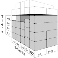
A container vessel normally has a 1.000-14.000 Twenty-Foot Equivalent Unit (TEU) capacity. A vessel is made up of a number of bays, which are collections of stacks of containers. Each stack has a height and weight limit that depends on the position of the stack. Each bay is divided into an on and below deck area separated by one or more hatch-lid covers. Each container stack is composed of vertically arranged groups of cells. Each cell is 40 feet long, 8 feet wide and 8.6 feet high and can hold one 40’ container or two 20’ containers. When holding two 20’ containers, they are said to be placed in theaftandforeTEU slot. If instead a 40’ container is placed in the cell, it is said to be placed in a Forty-Foot Equivalent Unit (FEU) slot. A location is a bay section below deck comprised of the slots under a hatch-lid cover. A bay has two to four of these depending on the number of hatch covers and for a typical large deep sea vessel, they have between 2 and 65 cells. Figure 1 shows a typical physical arrangement of containers in a location.
[image:2.595.306.557.53.103.2]The position of a container is given by its bay, stack, and tier number. The tier number defines its vertical position in
Fig. 1. A typical arrangement of containers in a location.
20’ Bay No. 40’ Bay No. 37 35
36 33 31
32 29 27
28 23 24 25 2119
20 17 15
16 13 11
12 09 07
08 03 05
04 01 39
41 40 45 43
44 49 47
48
Hatch−cover
Below deck area of bay
[image:2.595.109.211.658.759.2]On deck area of bay
Fig. 2. Layout and numbering of bays of a container vessel.
its stack. It is normal to use even numbers for FEU stacks and odd numbers for TEU stacks. The bays and cells of a container vessel are shown in Figure 2.
III. PROBLEMSTATEMENT
The representative problem we focus on is to stow or re-arrange a set of containers in a single location. Moving containers between locations is outside the scope of this paper but is a topic for future work. It requires that we also take stability and stress moment limits into account as well as potential increase in the port stay due to uneven distribution of container moves over bays. The subset of constraints that we model is described below.
1) One container must be placed in one slot, and in one slot only. Slots can only hold one container.
2) 40’ containers cannot be placed in a TEU slot and 20’ containers cannot be placed in a FEU slot.
3) The FEU slot of a cell occupies the same space as the TEU slots, so there can be no container in the TEU slots if a container is placed in the FEU slot and vice versa.
4) A 20’ container cannot stand on top of a 40’ container. 5) A container must have support from below.
6) When placing 20’ containers, the containers must be placed ‘evenly’, i.e. the number of containers in one TEU stack cannot exceed the number of containers in the other TEU stack with more than one.
7) For each stack, the sum of the weight of the containers must be within the weight limit of the stack.
8) Overstowage will not be allowed at all, so one con-tainer cannot be placed on top of a concon-tainer having a lower (earlier) discharge port.
9) Reefer containers cannot be placed in non-reefer slots. Notice that we do not consider the height of containers since height constraints are similar to weight constraints. We also do not model OOG, IMO and pallet-wide containers since the stacking rules associated with them are similar to the overstowage rule and the no 20’ above 40’ rule. Also notice that we model an objective of having no overstows indirectly as a constraint. Alternatively a limited number of overstows could be allowed. It is easy to show by a reduction from bin packing that determining feasibility of this problem is NP-complete [3]. Finding solutions without overstowage is also NP-complete by a reduction from coloring of circle graphs if stacks are uncapacitated [1].
IV. RELATEDWORK
performed modification has lead to an invalid plan rather than pre-computing the set of feasible modifications that the SC can choose from. All previous academic work has focused on optimization algorithms for generating a single stowage plan. Multi-phase approaches decompose the prob-lem hierarchically. 2-phase [13], [14], [15], [2] and 3-phase approaches [6], [7] are currently the most successful in terms of model accuracy and scalability. Single-phase approaches represent the stowage planning problem (or parts of it) in a single optimization model. Approaches applied include IP [16], [17], [18], [19], CP [20], [21], GA [22], [23]), SA [24], placement heuristics [25], 3D-packing [26]), simulation [27] , and case-based methods [28].
V. SOLUTIONAPPROACH
Aconfiguration problemC is formally defined as a triple
C= (X, D, F), whereX is a set of variablesx1, x2, . . . , xn,
Dis the Cartesian product of their finite domainsD1×D2× · · · ×Dn, and F =f1, f2, . . . , fm is a set of propositional
formulas specifying conditions that the variable assignments must satisfy.
A solution to a configuration problem is an assignment of the variables xi = vi, where vi ∈ Di for 1 ≤ i ≤ n that
satisfies all the formulas in F. An interactive configurator is a decision support tool that efficiently guides users to a desirable assignment. The configurator takes the set of variables X, their finite domains D and a set of rules F
as input. The configurator initially has an empty set of assignments. In each iteration, the invalid values of the domains of unassigned variables are removed such that each value in the domain of a variable is part of at least one valid assignment. The user then selects a preferred value of any unassigned variable. The algorithm terminates when all the variables are assigned. Pseudo code of the configurator is shown in Algorithm 1. As in our case where the user may only want to make a few changes to a given assignment, it is easy to change the algorithm to start with a partial assignment instead of an empty assignment. The algorithm is complete since the user can choose freely between any of the valid assignments, and it is backtrack-free since the user cannot choose a variable assignment for which no valid complete assignment exists, and is therefore never forced to go back and choose differently.
R←Compile(C)
1
while|R|>1 do
2
choose(xi=v)∈Valid-Assignments(R)
3
R←R|xi=v 4
end
5
Algorithm 1: Configurator.
BDD-based configuration [9] uses a BDD to representR
in order to compute valid assignments efficiently. In practice, the configurator algorithm is then a two phase approach. The first phase is an offline phase where the BDD is compiled and the second phase uses this BDD for fast complete inference. The advantage is that the worst case inference time in the online phase only grows polynomially with the size of the BDD and is often negligible.
A BDD is a rooted directed acyclic graph that is a compact representation of the decision tree of a Boolean function. It
has one or two terminal nodes,0and1, and a set of internal nodes associated with the variables of the function. Each internal node has a high and a low edge. For a particular assignment of the variables, the value of the function is determined by traversing the BDD from the root node to a terminal node by recursively following the high edge, if the associated variable is true, and the low edge, if the associated variable is false. The value of the function is
true, if the reached terminal node is1 and otherwisefalse. Figure 3 shows an example. Every path in the graph respects
0 1
x
x2 1
Fig. 3. A BDD of the functionf(x1, x2) =x1∨x2using orderx1≺x2. High and low edges are drawn with solid and dashed lines, respectively.
a linear ordering of the variables and to get small BDDs, it is important that variables that depend on each other are close in the ordering. Modern BDD packages represent sets of BDDs compactly as a single multi-rooted BDD. All Boolean functions can be carried out in polynomial time. Thus, BDDs are well suited for building fast inference systems for propositional logic. For a comprehensive introduction to BDDs, we refer the reader to [11], [29], [30].
We now illustrate BDD-based configuration on the small example shown in Figure 4. The problem is to place three
0 1 2 3
R
1 2
3 4R R
Fig. 4. A bay stowage example with 4 slots (left) and 3 containers (right).
standard 40’ containers in a FEU bay with two stacks each with two slots. We assume that one of the containers is a reefer container and two of the slots are reefer slots (both indicated by “R” in the figure). We also assume that containers and slots are numbered as shown in the figure and that slots assigned to0(⊥) do not hold any container.
We use four variablesx1,x2,x3, andx4each with domain {0,1,2,3}. An assignment xi = vi denotes that the slot
with numberihold the container with numbervi. The set of
propositional formulas shown below defines the set of valid assignments.
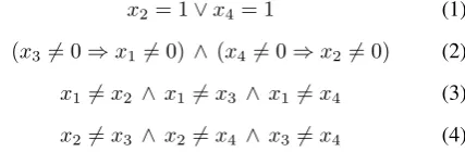
x2= 1∨x4= 1 (1)
(x36= 0⇒x16= 0) ∧(x46= 0⇒x26= 0) (2)
x16=x2 ∧x1=6 x3 ∧x16=x4 (3)
x26=x3 ∧x2=6 x4 ∧x36=x4 (4)
Constraint (1) ensures that the reefer container is placed in a reefer slot, constraint (2) ensures that no container hangs in the air. Finally, constraint (3) and (4) ensure that one container at most can be assigned to one slot.
[image:3.595.334.548.616.686.2]the two Boolean variables of xi. In a binary encoding of
the domain of xi, x1i and x0i represents the value of bit 1
and 0 ofxi, respectively. Thus, the propositional expression
x1
i∧ ¬x0i represents the constraintxi= 2and so on. We can
now translate constraint (1 - 4) to propositional formulas. In the offline phase of the BDD-based configurator (line 1 of Algorithm 1), a single BDD is built equal to the conjunction of the propositional formulas. The resulting BDD of our example is shown in Figure 5 (left). For
[image:4.595.56.282.177.385.2]x
1 3x
1 3x
1 3 1 3 1 3x
x
1
x
1 4 4 1x
x
x
x
x
3 41
x
1 4x
4 0 4x
0 4x
0 4x
0 4x
0 3x
0 3x
0 3x
1 2 1 2x
1 2x
0 2x
0 2x
1 1x
1 1 1 1 2x
0 4x
0 4x
0 4x
0 3x
0 3x
0 1x
0 2x
0 2x
1 1x
1 1x
0 1x
1 2x
x
x
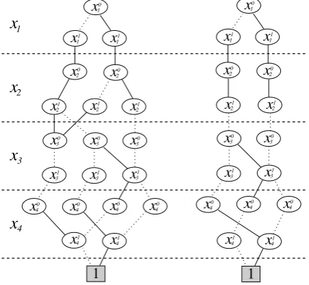
2 1Fig. 5. Left: BDDRof the conjunction of the constraints (1-4). Right: Reduced BDDR∧(x2= 1).
clarity, we do not draw edges leading to terminal 0. Each of the six distinct paths leading to terminal 1 corresponds to one of the six possible arrangements of the containers shown in Figure 6. Each iteration of the online phase of the
2
3 R 2
3
R 2 3
R 3 2 R 2 3 R 3 2 R
Fig. 6. The six valid container configurations of the example shown in Figure 4. The four shaded configurations are represented by the BDD shown in Figure 5 (right) withx2= 1.
BDD-based configurator (line 2-5) starts with a computation of the valid assignments of the remaining configurations represented by the BDD R. Since the variables are ordered in layers from top to bottom inR, it is possible to compute their valid assignments by probing it in justO(Pn
i=1|Di|Vi),
whereViis the number of BDD nodes in the layer of variable
xi and |Di| is the size of the original domain of xi [31].
Unless the BDD representing a configuration problem grows very large, the time needed to compute valid assignments is a few milliseconds and hardly noticed by the user. The result of the valid assignments computation is a reduced domain for each variable. If there is only a single value left for a variable there is no further decisions to make for it and it is assigned automatically by the system. The user then chooses one of the possible values from the reduced domains andRis restricted to this choice byR←R∧(xi=vi). Assume that
the user chooses x2 = 1in the first iteration. The reduced
BDDR is shown in Figure 5 (right).
Due to the speed of the valid assignments computation, BDD-based configuration enables the user to navigate fast in the configuration space without having to worry about the feasibility of the partial configuration. This allows SCs to focus on achieving their preferred stowage when re-arranging containers in a location.
In order to define a configurator for re-arranging containers in a location as described in Section III, we choose slots as decision variablesX with containers as domainsD and introduce the following:
• A set of stacksS={1, . . . , s},
• A set of tiersTσ={tσ, . . . , t}of stack σ∈S,
• A set of slots (the variables)X ={cFTσ,τ, cATσ,τ, cFσ,τ|σ∈
S, τ ∈Tσ} where FT stands for Fore TEU, AT stands
for Aft TEU and F stands for FEU. For example; cFT
2,4
is the fore TEU slot in stack 2 and tier 4.
• A set of containers (the domains) {D1, D2, . . . , Dn},
where Di = {0,1, . . . , c} and c is the number of
containers. The value 0 means that no container is placed in the slot.
• A set of constraintsF defined below.
Some constraints can be modeled by reducing the domains of the slot variables. These include that TEU slots cannot contain 40’ containers, and FEU slots cannot contain 20’ containers. Also, that reefer containers cannot be placed in non-reefer slots. To simplify the presentation, we assume that the Boolean values true and f alse can also represent the numericals1and0.
If there is a container in the fore TEU or aft TEU slot, no containers can be placed in the FEU slot, (since they are occupying the same space). The constraint of the rule works both ways
^
σ∈S
^
τ∈Tσ
cF
σ,τ = 0∨(c
FT
σ,τ = 0∧c
AT
σ,τ = 0). (5)
A 20’ container cannot stand on top of a 40’ container
^
σ∈S
^
τ∈Tσ\{t}
cF
σ,τ 6= 0⇒(c
FT
σ,τ+1= 0∧c
AT
σ,τ+1= 0).
(6) When placing 20’ containers, the containers must be placed ‘evenly’
^
σ∈S
^
τ∈Tσ\{t}
(cFT
σ,τ = 0⇒cATσ,τ+1= 0)∧
(cAT
σ,τ = 0⇒cFTσ,τ+1= 0).
(7)
Also, containers must have support from below
^
σ∈S
^
τ∈Tσ\{t}
(cFT
σ,τ = 0⇒cFTσ,τ+1= 0)∧
(cAT
σ,τ = 0⇒cATσ,τ+1= 0)∧
cF
σ,τ = 0∧(cFTσ,τ = 0∨cATσ,τ = 0)⇒
cF
σ,τ+1= 0
.
(8) The expressions (6), (7), and (8) can be rewritten as
^
σ∈S
^
τ∈Tσ\{t}
(cFT
σ,τ = 0∨cATσ,τ = 0)⇒
(cFT
σ,τ+1= 0∧cATσ,τ+1= 0)
∧
cF
σ,τ = 0∧(c
FT
σ,τ = 0∨c
AT
σ,τ = 0)⇒
cF
σ,τ+1= 0
,
[image:4.595.303.552.398.815.2]or in plain words: If either of the TEU slots are empty, both of the TEU slots above must be empty (this takes care of the ‘no containers hanging in the air’ and ‘evenly stacking’ constraints, and given (5), also the ‘no 20’ on top of 40’ constraint). If the FEU slot is also empty, the FEU slot above must be empty (contrary it would hang in the air).
One container must be placed in one slot, and in one slot only
^
χ∈C
X
σ∈S
X
τ∈Tσ
(cFT
σ,τ =χ)+(c
AT
σ,τ =χ)+(c
F
σ,τ=χ)
= 1,
(10) where C = {1,2, . . . , c} is the set of containers. For the weight constraints, let w(χ) denote the weight of container
χ withw(0) = 0. Further, letwlimσ be the weight limit of
stackσ. We then require
^
σ∈S
X
τ∈Tσ
w(cFT
σ,τ) +w(c
AT
σ,τ) +w(c
F
σ,τ)
≤wlimσ. (11)
For the overstow constraint, let d(χ) denote the discharge port of container χ, where the discharge port 1 is the first downstream port to visit, discharge port2is the second etc.. We have d(0) = 0. The requirement is that the discharge port of the containers in each stack are ordered asscendingly from top to bottom
^
σ∈S
^
τ∈Tσ\{t}
min{d(cFT
σ,τ), d(cATσ,τ), d(cFσ,τ)} ≥
max{d(cFT
σ,τ+1), d(cATσ,τ+1), d(cFσ,τ+1)}.
(12)
VI. COMPUTATIONALRESULTS
The configurator was implemented using the BDD-based configuration engine CLab [10]. Upon start-up, the program makes the configuration file for CLab, and CLab compiles it and returns the corresponding BDD of the configuration problem. Then a GUI, based on the Qt UI framework [32] emerges, as shown in Figure 7. The cells are divided into FTEU, ATEU and FEU slots. Long container buttons at the bottom of the screen represent 40’ containers, short buttons represent 20’ containers. The color shade of containers is determined by their discharge port or weight. Slots and containers with an ‘R’ are reefer slots and containers, re-spectively.
When the user clicks on a slot or a container, the color of the container or slot becomes red if the placement is illegal, or green otherwise, as shown in Figure 8. When the user clicks on a slot, the program returns the slot’s domain (the legal containers). When the user clicks on a container, the program returns the variables (slots) having the container in its domain. By clicking on a green (legal) container or slot, the container is placed in the slot, and the color turns into grey (the shade is still determined by the discharge port or weight of the container). This can be undone by clicking on the grey slot or container or the ‘undo’ button. Notice that when using groups (explained in the next section), a container (group) does not get a grey color until all the containers in the group have been placed.
Slots that due to the constraints cannot have any containers placed in them, are colored white. If the reason for this is that there is (or has to be) a container in the overlapping FEU slot (if the slot is an FTEU or ATEU slot) or in the
overlapping FTEU or ATEU slot (if the slot is an FEU slot), this is marked with a black dot.
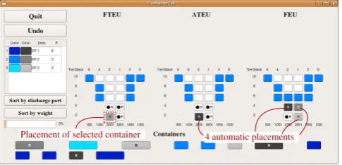
After each restriction of the BDD, the program searches for container placements that are obliged to happen. If found, these are automatically carried out. This will for example happen when the 20’ container selected in Figure 8 is placed incFT
[image:5.595.305.547.153.271.2]2,2. The result is shown in Figure 9. Notice that a partial
Fig. 7. Screenshot of GUI after start-up (12 containers, 18 cells). The darker blue / shaded, the heavier container.
[image:5.595.305.548.328.446.2]Selected container
Fig. 8. A 25 ton 20’ non-reefer container with discharge port 3 selected. GUI shows valid (green / light shaded) and invalid (red / dark shaded) slots.
4 automatic placements Placement of selected container
Fig. 9. A 25 ton 20’ non-reefer container with discharge port 3 placed in reefer slotcFT
2,2. GUI has made 4 automatic placements.
plan does not have to satisfy all constraints (e.g., that the containers form physical stacks). The requirement is that a partial plan can be extended to a complete plan that does satisfy them.
[image:5.595.306.549.503.620.2]than exactly which container it is. This breaks symmetry, since the model now ignores the ordering of the containers within each group.
Most of the characteristics of a container are discrete and finite, with only a small number of possible values. But the weight of a container is a continuous value. So, strictly speaking, two otherwise similar containers with a weight of 25.676 and 25.677 tons are not similar and can not be put in the same group. In order to be able to group containers at all, we have to relax the problem.
The relaxation we consider is to allow grouping of con-tainers with ‘almost equal’ weight. The concon-tainers in a group will get their weightw(χ)changed to the weight of the group the containers belong to, defined as wg(χ). This value must
be at least equal to the weight of the heaviest container in the group, to avoid underestimating the weight of a stack. We define ‘weight loss’; i.e. the total weight overestimation to beP
χ∈Cwg(χ)−w(χ).
The easiest way to group the containers is to have pre-defined weight intervals. But it is obvious that this solution is not an optimal one. Consider a pre-defined grouping with a interval of 2 tons. A set of 4 containers having weights of 23.999, 24.001, 25.999 and 26.001 tons could lead to a solution that is far from optimal. Another approach is to find a solution with minimum weight loss given a limit on the number container groups. This problem can be solved using dynamic programming. For a detailed description of the algorithm, we refer the reader to [33].
b) Scalability: The purpose of the stowage configurator is to support re-assignment of containers in individual loca-tions in the last phase of the stowage planning process where the SC is either checking low-level stacking rules of his or her own plan or is correcting a stowage plan generated offline by an optimization algorithm. In each case, the plan will typically be correct wrt. high-level constraints and objectives such as vessel stability, lid-overstowage, and minimization of crane makespan. For that reason any low-level issues should be solved without moving containers between locations since this may break the achieved high-level solution.
A configurator should be built for each location. This can either be done online by the SC high-lighting a storage area that a configurator is then built over or offline as a part of running an optimization algorithm. For this to be practical it is necessary that an initial BDD can be built in reasonable time (<20 seconds) and that the resulting BDD is small enough for the valid assignment computation time to be experienced as instantaneous (< 10 million nodes). To investigate this, we carried out performance tests on a machine with the level of computing power that can be assumed to be available for SCs (HP 6715b laptop having a AMD Turion X2 2 Ghz processor and 3 GB RAM).
We first consider our initial model without symmetry breaking where each container is represented independently. The size of the initial BDD as a function of the number of cells and containers is shown in Figure 10. The build time in these experiments varies between 1.5 and 105 seconds and is strongly correlated with the size of the generated BDD. The initial BDD and the computation time grows moderately with the number of cells but fast with the number of containers.
[image:6.595.307.547.559.709.2]Our initial model does not scale sufficiently. The size of a location in the order of 2 to 65 cells, but already at 18
Fig. 10. Size of initial BDD as a function of the number of cells and containers.
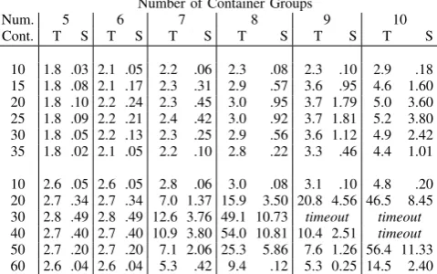
cells and containers is the size of the BDD larger than two million nodes and takes more than 100 seconds to generate. By grouping the containers, we only approximate con-tainer weights. All other attributes are still accurate. More-over, the approximation is conservative such that valid con-figurations still satisfy the weight constraints. In our second experiment, we vary the number of containers and container groups. We consider two locations both with 6 stacks. The first has 36 cells and 16 reefers slots. The second has 60 cells and 15 reefers slots. We place a mix of 20’, 40’ and reefer containers with typical weights and three different discharge ports. Compared to real instances, these are actually hard. It is very rare to mix 20’ and 40’ containers with different reefer features and more than two discharge ports in a single location. The reason is that we do not expect SCs to need configuration support unless the stowage problem is combinatorially challenging. Table I shows the size and build time of the initial BDD as a function of number of containers to stow (rows) and number of container groups (columns).
TABLE I
BDDBUILD TIME AND SIZE AS A FUNCTION OF NUMBER OF CONTAINER GROUPS AND CONTAINERS TO STOW. THE FIRST COL. (NUM. CONT.)IS
THE NUMBER OF CONTAINERS TO STOW. FOR EACH NUMBER OF CONTAINER GROUPS(5-10),COL. TIS THE BUILD TIME IN SECONDS (TIMEOUT3MIN.)ANDSIS THE SIZE IN MILLIONS OF NODES. THE TOP
AND BOTTOM TABLE SHOW RESULTS FOR THE36AND60CELL LOCATION,RESPECTIVELY.
Number of Container Groups
Num. 5 6 7 8 9 10
Cont. T S T S T S T S T S T S
10 1.8 .03 2.1 .05 2.2 .06 2.3 .08 2.3 .10 2.9 .18 15 1.8 .08 2.1 .17 2.3 .31 2.9 .57 3.6 .95 4.6 1.60 20 1.8 .10 2.2 .24 2.3 .45 3.0 .95 3.7 1.79 5.0 3.60 25 1.8 .09 2.2 .21 2.4 .42 3.0 .92 3.7 1.81 5.2 3.80 30 1.8 .05 2.2 .13 2.3 .25 2.9 .56 3.6 1.12 4.9 2.42 35 1.8 .02 2.1 .05 2.2 .10 2.8 .22 3.3 .46 4.4 1.01
10 2.6 .05 2.6 .05 2.8 .06 3.0 .08 3.1 .10 4.8 .20 20 2.7 .34 2.7 .34 7.0 1.37 15.9 3.50 20.8 4.56 46.5 8.45 30 2.8 .49 2.8 .49 12.6 3.76 49.1 10.73 timeout timeout
40 2.7 .40 2.7 .40 10.9 3.80 54.0 10.81 10.4 2.51 timeout
50 2.7 .20 2.7 .20 7.1 2.06 25.3 5.86 7.6 1.26 56.4 11.33 60 2.6 .04 2.6 .04 5.3 .42 9.4 .12 5.3 0.25 14.5 2.40
A high-level objective of stowage planning is to cluster similar containers in bays. For that reason, containers with identical attributes often will contain the same goods and therefore approximately have the same weight. This means that even a minimal sized weight grouping often will have a total weight overestimation that is negligible in practice.
For the 36 cell location, reasonably sized BDDs can be computed in less than 10 seconds for up to 10 groups. For the 60 cell location, the computation time becomes too long when using more than 7 groups, but interestingly only if stowing about half of the 60 containers. Since 10 groups is a lot even for locations with 60 cells, the experimental results of the grouping model shows that it can scale to the size of problems considered by SCs.
VII. CONCLUSION
In this, paper we have introduced an approach for in-teractive decision support for stowing containers in bay sections below deck. The approach uses a fast and complete inference method where a BDD representing the complete configuration space of the containers is built offline and used online to guide an SC to a desired feasible stowage plan.
Our computational results show that the approach scales to real-sized instances when breaking symmetries among similar containers. Our GUI further demonstrates that it is possible to integrate the configurator in a visual tool that is easy to use for SCs.
Future work includes applying recent powerful SAT-based configuration approaches [12] and model all container types. We also want to extend to modifying complete stowage plans where moves between locations are possible. It is also interesting to investigate to what extend configuration techniques can be applied to guide SCs in solution pools generated by standard optimization tools.
REFERENCES
[1] M. Avriel, M. Penn, and N. Shpirer, “Container ship stowage problem: Complexity and connection to the coloring of circle graphs,”Discrete
Applied Mathematics, vol. 103, pp. 271–279, 2000.
[2] D. Pacino, A. Delgado, R. M. Jensen, and T. Bebbington, “Fast generation of near-optimal plans for eco-efficient stowage of large container vessels,” inProceedings of the 2nd International Conference
on Computational Logistics (ICCL’11), ser. LNCS. Springer, 2011.
[3] A. Delgado, R. M. Jensen, K. Janstrup, T. H. Rose, and K. H. Andersen, “A constraint programming model for fast optimal stowage of container vessel bays,”European Journal of Operational Research, 2011, under revision.
[4] Navis, “PowerStow,” www.navis.com, 2011. [5] Interschalt, “Seacos,” www.interschalt.de, 2011.
[6] D. Ambrosino, D. Anghinolfi, M. Paolucci, and A. Sciomachen, “An experimental comparison of different heuristics for the master bay plan problem,” inProceedings of the 9th Int. Symposium on Experimental
Algorithms, 2010, pp. 314–325.
[7] M. Yoke, H. Low, X. Xiao, F. Liu, S. Y. Huang, W. J. Hsu, and Z. Li, “An automated stowage planning system for large containerships,”
in In Proceedings of the 4th Virtual Int. Conference on Intelligent
Production Machines and Systems, 2009.
[8] N. Guilbert and B. Paquin, “Container vessel stowage planning, Patent Publication US2010/0145501,” 2010.
[9] S. Subbarayan, R. M. Jensen, T. Hadzic, H. R. Andersen, J. Møller, and H. Hulgaard, “Comparing two implementations of a complete and backtrack-free interactive configurator,” inProceedings of the CP-04
Workshop on CSP Techniques with Immediate Application. Springer,
2004, pp. 97–111.
[10] R. M. Jensen, “CLab: a C++ library for fast backtrack-free interactive product configuration,” in In Proceedings of the 10th International Conference on Principles and Practice of Constraint Programming
(CP-04). Springer, 2004, p. 816.
[11] R. E. Bryant, “Graph-based algorithms for boolean function manipu-lation,”IEEE Transactions on Computers, vol. 8, pp. 677–691, 1986. [12] M. Janota, “SAT solving in interactive configuration,” Ph.D.
disserta-tion, University College Dublin, November 2010.
[13] I. D. Wilson and P. A. Roach, “Principles of combinatorial optimiza-tion applied to container-ship stowage planning,”Journal of Heuristics, vol. 5, pp. 403–418, 1999.
[14] J. G. Kang and Y. D. Kim, “Stowage planning in maritime container transportation,”Journal of the Operational Research Society, vol. 53, pp. 415–426, 2002.
[15] W.-Y. Zhang, Y. Lin, and Z.-S. Ji, “Model and algorithm for container ship stowage planning based on bin-packing problem,” Journal of
Marine Science and Application, vol. 4, no. 3, 2005.
[16] R. C. Botter and M. A. Brinati, “Stowage container planning: A model for getting an optimal solution,” inProceedings of the Seventh International Conference on Computer Applications in the Automation
of Shipyard Operation and Ship Design. North-Holland Publishing
Co., 1992, pp. 217–229.
[17] D. Ambrosino and A. Sciomachen, “Impact of yard organization on the master bay planning problem,”Maritime Economics and Logistics, no. 5, pp. 285–300, 2003.
[18] P. Giemesch and A. Jellinghaus, “Optimization models for the contain-ership stowage problem,” Proceedings of the International Conference of the German Operations Research Society, 2003.
[19] F. Li, C. Tian, R. Cao, and W. Ding, “An integer programming for container stowage problem,” inProceedings of the Int. Conference on
Computational Science, Part I. Springer, 2008, pp. 853–862, LNCS
5101.
[20] D. Ambrosino and A. Sciomachen, “A constraint satisfaction approach for master bay plans,”Maritime Engineering and Ports, vol. 36, pp. 175–184, 1998.
[21] A. Delgado, R. M. Jensen, and C. Schulte, “Generating optimal stowage plans for container vessel bays,” inProceedings of the 15th Int. Conf. on Principles and Practice of Constraint Programming (CP-09), ser. LNCS Series, vol. 5732, 2009, pp. 6–20.
[22] Y. Davidor and M. Avihail, “A method for determining a vessel stowage plan, Patent Publication WO9735266,” 1996.
[23] O. Dubrovsky, G. Levitin, and M. Penn, “A genetic algorithm with a compact solution encoding for the container ship stowage problem,”
Journal of Heuristics, vol. 8, pp. 585–599, 2002.
[24] M. Flor, “Heuristic algorithms for solving the container ship stowage problem,” Master’s thesis, Technion, Haifa, Isreal, 1998.
[25] M. Avriel, M. Penn, N. Shpirer, and S. Witteboon, “Stowage plan-ning for container ships to reduce the number of shifts,” Annals of
Operations Research, vol. 76, pp. 55–71, 1998.
[26] A. Sciomachen and A. Tanfani, “The master bay plan problem: a solution method based on its connection to the three-dimensional bin packing problem,”IMA Journal of Management Mathematics, vol. 14, pp. 251–269, 2003.
[27] W. C. Aye, M. Y. H. Low, H. S. Ying, H. W. Jing, and Z. Min, “Visualization and simulation tool for automated stowage plan gener-ation system,” inProceedings of the International MultiConference of
Engineers and Computer Scientists 2010 (IMECS 2010), vol. 2, Hong
Kong, 2010, pp. 1013–1019.
[28] S. Nugroho, “Case-based stowage planning for container ships,” in
The Int. Logistics Congress, 2004.
[29] C. Meinel and T. Theobald,Algorithms and Data Structures in VLSI
Design. Springer, 1998.
[30] I. Wegener, Branching Programs and Binary Decision Diagrams. Society for Industrial and Applied Mathematics (SIAM), 2000. [31] T. Hadzic, R. M. Jensen, and H. R. Andersen, “Calculating valid
domains for BDD-based interactive configuration,” 2005, IT University of Copenhagen.
[32] Nokia Corporation, “Qt,” qt.nokia.com, 2010.