Online Full Text

(1)



Abstract—A power system at a given operating state and subjected to a given disturbance is voltage stable if the voltages near loads approach post-disturbance equilibrium values. In this paper, by using the energy function that maps the energy variation of the system, the effect of the slow chance of the system is analyzed and thus the system’s energy level changes’ effects on the system’s stability is shown by using MATHCAD program. It is demonstrated that the stored energy measure is an indicator of the closeness of the operating point to the instability region of the system.

Index Terms—Energy function, Lyapunov’s second method, The variable gradient method, Voltage stability

NOMENCLATURE

δ Load angle in radians

V Load voltage in p.u. Em Generator voltage in p.u.

E0 Infinite bus or slack bus voltage in p.u.

Ym Generator admittance in p.u.

Y0 Infinite bus or slack bus admittance in p.u.

δm Generator rotor angle in radians

C Compensated load capacitor in p.u. θm Generator admittance angle in degrees

θ0 Infinite bus admittance angle in degrees

M Generator inertia in p.u.

D Damping coefficient

Pm Mechanical power in p.u.

Kpw, Kpv Constant parameters

Kqw, Kqv, Kqv2 Constant parameters I. INTRODUCTION

INCE 1920s, electric power system stability has been considered as an important problem in terms of reliable system operation [1], [2]. The concept of voltage stability is expressed as the ability of keeping voltages’ magnitudes of load buses, under both in steady state voltage stability and transient voltage stability conditions, within the specific operating limitations [3].

In the cases of not making voltage control and increase

Manuscript submitted February 21, 2011

A. Cifci is currently a lecturer with the Department of Electrical, Mehmet Akif Ersoy University, 15100, Burdur, Turkey (corresponding author to provide phone: +902482134583; fax: +902482345604; e-mail: [email protected]).

Y. Uyaroglu is currently an Assist. Prof. with the Department of Electrical and Electronics Engineering, Sakarya University, 54050, Sakarya, Turkey (e-mail: [email protected]).

A. T. Hocaoglu is currently a director with the Directorate of Electrotechnical Laboratory, Turkish Standards Institution, 41420, Gebze, Turkey (e-mail: [email protected]).

the load due to disabling, for any reason, the elements such as generator, line, transformer, bus etc if an uncontrolled voltage drop occurs, then there appears power system instability. The main reason of the voltage instability is that in the overloaded systems the system can not ensure the reactive energy needed by the system to keep voltage values in a certain amount [4]–[7]. Other reasons are generator reactive power limits, load characteristics, characteristics of load tap changer transformers, characteristics of reactive power compensation devices and behaviour of voltage control devices [8].Voltage stability and collapses began to play a significant role in power system analysis and control as a result of energy system collapses in various places of the world such as Egypt [9], Chile [10], The United States and Canada [11], [12].

This study is organized as follows respectively. Section II outlines the main idea of Lyapunov stability analysis. Section III examines a single-machine infinite-bus power system’s energy function. Section IV presents simulation results of energy function analysis. Finally conclusions are given in Section V.

II. LYAPUNOV STABILITY ANALYSIS

The constant exponents can be used in the study of nonlinear differential equations’ stability was first shown by a Russian mathematician, Sonya Kovalevskaya, in 1889. Later in 1892 Kovalevskaya’s study was developed by another Russian mathematician, Alexandr Mikhailovich Lyapunov.

Lyapunov’s second method (also called Lyapunov’s direct method) provides us with studying the stability of the system concerning on the dynamic system before finding the solution of differential equation. The second method is appropriate for the voltage stability of nonlinear systems which do not have accurate solutions. This method is the most common one in terms of the determination of stability conditions of time-dependent nonlinear systems and could be applied to all known systems.

Stability Analysis of Nonlinear Systems

Voltage stability of nonlinear systems is regional. Hence, Lyapunov function which obtains sufficient stability conditions in the largest region around the origin is searched for.

Some methods which arise from Lyapunov’s second method are proper to examine the stability of nonlinear systems. One of them is the variable gradient method which is used for the generalization of Lyapunov functions.

Energy Function Analysis of a Single-Machine

Infinite-Bus Power System

A. Cifci, Y. Uyaroglu, and A. T. Hocaoglu

(2)

The Variable Gradient Method

There are no generally applicable methods for finding Lyapunov functions. The variable gradient method is a formal approach to constructing Lyapunov functions. The variable gradient method assumes a certain form for the gradient of an unknown Lyapunov function, and then finding the Lyapunov function itself by integrating the assumed gradient [13].

Consider a nonlinear dynamical system described by

) t , x ( f

x (1) f: n×1 nonlinear vector function

x: n×1 state vector

n: numbers of states, order of the systems

Accept an equilibrium point at the origin of the space. Denote a test Lyapunov function by using V. Assume that in (1), V is x’s open function but not t’s. Then,

n n 2

2 1 1

x x

V ... x x

V x x V

V   

    

   

 (2)

can be written. Hence,

x ) V (

V  * (3)

In (3), (V)* isV’s transpose. The gradient of V, denoted by V as follows:

     

 

     

 

 



       

 

       

 

   

 

n 1

V . . . V

x V . . . x V

V (4)

V

 ’s line integral can be expressed by



 

x

0 *

dx ) V (

V (5)

In (5), integral’s upper limit does not point that V is a vector magnitude, but integral is prefer to line integral of a random point (x1,x2,…,xn) at the space. This integral can be

done separately from integration method.

Investigation of Lyapunov Function Using Gradient System A special class of dynamical system is particularly well suited to the Lyapunov method. This system arises from the gradient of a function [14]. A gradient dynamical system is given as

) x , x ( v A

x  0 (6)

In (6), v: nxn  can be a continuously differentiable.Anxn is defined as det(A)≠0 and

v(x,x0)=0 for x=x0. If v(x,x0)’s Hessian is completely

positive definite at x0, equilibrium point is asymptotically

stable at x0.

Lyapunov function is given as



f()



d

) x ( V

T x

x₀



 (7)

Lyapunov function which is given above will be used in order to find the single-machine infinite-bus power system’s energy function.

III. ENERGY FUNCTION OF A SINGLE-MACHINE INFINITE -BUS POWER SYSTEM

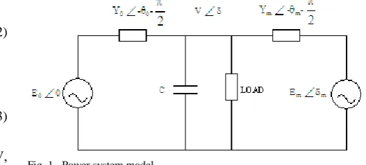
[image:2.595.285.549.276.395.2]

We consider the power system model shown in Fig. 1, which is taken from [15].

Fig. 1. Power system model.

This system consists of a load bus and two generator buses. One of the generator busses is treated as a slack bus. The load is modelled by a simplified induction motor in parallel with a constant P-Q load and constant impedance. The load also includes a fixed capacitor C to raise the voltage up to near 1.0 per unit [15]. The network, load and generator parameters have been presented in the Appendix. First-order differential equations are expressed which show power system model’s equations of state as follow [16].

w

m

 ₍₈₎ m

m 2 m m m m

m

m EVY sin( ) E Y sin

P Dw w

M       (9) 1

0 2

2 qv qv

qw K V K V Q Q Q

K      (10)

) P P P ( K ) Q Q Q ( K

... V ) K K K K ( V K K V K TK

1 0 qw 1

0 pw

pv qw qv pw 2 2 qv pw pv qw

  

  

 





(11)

The system differential equations above can be written again under the condition that generator mechanical power is equivalent to active load requirement (Pm=Pl).

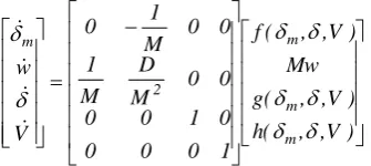
) V , , ( f M

1 Mw M

D

w  ₂   m (12)

Mw M

1

m

 ₍₁₃₎

) V , , (

g  m

  ₍₁₄₎

) V , , ( h

(3)

)) sin( Y E ) sin( VY E P ( ) V , , (

f m m

2 m m m m m m

m    



      (16)

) Q Q Q V K V K ( K 1 ) V , , (

g qv 0 1

2 2 qv qw

m      



 (17)

)) P P P ( K ) Q Q Q ( K V ) K K ... Kqv K ( V K K ( K TK 1 ) V , , ( h 1 0 qw 1 0 pw pv qw pw 2 2 qv pw pv qw m             (18)

The system differential equations expressed by the equations (8), (9), (10), and (11) are the definition of the simple system that involves highly complicated load modelling at around the high voltage operating point. Defining Gradient System to the Form of Lyapunov Function for a Simple Power System

The derivation of Lyapunov Function for the system in Fig. 1, equations (12), (13), (14) and (15) could be determined as                             _                ) V , , ( h ) V , , ( g Mw ) V , , ( f 1 0 0 0 0 1 0 0 0 0 M D M 1 0 0 M 1 0 V w m m m 2 m             (19)

The equation (19) for the system defined in (8), (9), (10) and (11) equations, is an alternative definition for this system’s dynamics.

For the (w0,δm0,δ0,V0)’s equilibrium point, a candidate

energy function which is seen on the right of the (19) equation ((4x1) gradient matrix seen on the right of the (19) equation) is obtained and therefore it can be used in (7) equation. The candidate energy function can be written in (7) equation as



                         ) V , , , w ( ) V , , , w ( m T m m m m m 0 0 0 m 0 dV d d dw ) V , , ( h ) V , , ( g ) V , , ( f Mw ) V , , , w ( v             

 (20)

If f(w,δm,δ,V), g(w,δm,δ,V) ve h(w,δm,δ,V) are replaced on

(20) equation, the system’s energy function is obtained [17]. The equilibrium point is (w*,δm*,δ*,V*)=(0.0,0.3,0.2,0.97).

IV. SIMULATION RESULTS OF A SINGLE-MACHINE INFINITE -BUS POWER SYSTEM

There are four important state variables in these analyses. These are the system frequency (w1), generator rotor angle

(δm), load angle (δ) and load voltage (V). The aim of these

analyses is to show what kind of effects the load would have over the whole energy of the power system. The generator rotor angle will be changed, beginning with zero and will be increased to 1.6 by 0.4 rise each turn in order to observe the system’s stability.

The sample of the energy function for the single-machine infinite-bus power system is given as follows:

a V a V a V 008 . 2 ) V , (

v



 3  ₂ 2  ₁  (21) When the sample of the energy function given above is equalized the system’s energy function which is obtained from (20) equation, a2, a1 and a are respectively obtained for

each case. The following cases are considered:

Case-1: Generator rotor angle δm=0 rad., system frequency

w=1 p.u

a2, a1 and a are respectively obtained as

) 209 . 0 cos( 4 ) 087 . 0 cos( ) 209 . 0 sin( 3 . 0 )... 087 . 0 sin( 075 . 0 907 . 14 426 . 2 a2                (22) ) 209 . 0 sin( 20 ) 087 . 0 sin( 5 )... 087 . 0 cos( 5 ) 213 . 0 cos( 5 8 . 2 405 . 0 a₁                 (23) ) 209 . 0 cos( 386 . 3 ) 087 . 0 cos( 846 . 0 )... 209 . 0 sin( 254 . 0 ) 087 . 0 sin( 063 . 0 3 . 1 336 . 1 a                 (24)

(a) (b)

Fig. 2. System’s stored energy for δm=0 (a) Two-dimensional representation (b) Three- dimensional representation.

The system's energy density is in the range of 0.6≤V≤1 and 1≤δ≤1.6, which is seen as in Fig. 2 and Table I. The system's energy density varies between 8 and 9 energy units around these points.

TABLEI

ENERGY MEASUREMENT FOR ΔM=0

δ Energy

Measurement

0 2,9 2,3 1,8 1,2 0,6 -0,1 -0,7 -1,3 -1,9 -2,4 -2,9 0,2 2,6 2,6 2,6 2,4 2,2 1,8 1,5 1,1 0,6 0,2 -0,3 0,4 2,2 2,8 3,2 3,5 3,6 3,6 3,5 3,3 3,1 2,7 2,3 0,6 1,6 2,7 3,6 4,3 4,8 5,2 5,4 5,4 5,3 5,0 4,7 0,8 0,9 2,5 3,8 4,9 5,8 6,4 6,8 7,1 7,1 7,0 6,7 1 0,0 2,1 3,8 5,2 6,4 7,2 7,9 8,3 8,4 8,3 8,0 1,2 -0,9 1,4 3,5 5,2 6,5 7,6 8,4 8,9 9,1 9,0 8,7 1,4 -2,0 0,7 2,9 4,8 6,3 7,5 8,3 8,8 9,0 8,9 8,4 1,6 -3,1 -0,3 2,1 4,1 5,6 6,8 7,6 8,0 8,1 7,8 7,2 1,8 -4,2 -1,3 1,1 3,0 4,6 5,6 6,3 6,5 6,4 5,8 4,9 V 0 0,1 0,2 0,3 0,4 0,5 0,6 0,7 0,8 0,9 1 For δm=0 rad. and w=1 p.u., Table I shows numerical

values of the energy function for different load angles and different load voltages.

Case-2: Generator rotor angle δm=0.4 rad., system

frequency w=1 p.u.

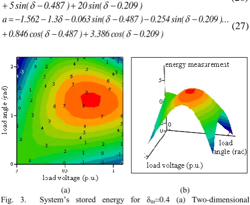
[image:3.595.48.216.291.366.2] [image:3.595.308.549.292.440.2] [image:3.595.304.553.530.673.2]

(4)

) 209 . 0 cos( 4 ) 487 . 0 cos( ) 209 . 0 sin( 3 . 0 )... 487 . 0 sin( 075 . 0 907 . 14 426 . 2 a2                (25) ) 209 . 0 sin( 20 ) 487 . 0 sin( 5 )... 313 . 0 cos( 5 ) 213 . 0 cos( 5 8 . 2 573 . 1 a1                (26) ) 209 . 0 cos( 386 . 3 ) 487 . 0 cos( 846 . 0 )... 209 . 0 sin( 254 . 0 ) 487 . 0 sin( 063 . 0 3 . 1 562 . 1 a                 (27)

(a) (b)

Fig. 3. System’s stored energy for δm=0.4 (a) Two-dimensional representation (b) Three- dimensional representation.

The system's energy density is in the range of 0.5≤V≤1 and 1≤δ≤1.6, which is seen as in Fig. 3 and Table II. The system's energy density varies between 7 and 8 energy units around these points.

TABLEII

ENERGY MEASUREMENT FOR ΔM=0.4

δ Energy

Measurement

0 2,6 2,1 1,5 1,0 0,4 -0,2 -0,8 -1,3 -1,9 -2,4 -2,8 0,2 2,4 2,4 2,3 2,1 1,9 1,5 1,1 0,7 0,3 -0,2 -0,7 0,4 2,0 2,6 2,9 3,1 3,2 3,2 3,0 2,8 2,4 2,0 1,5 0,6 1,5 2,5 3,4 4,0 4,4 4,6 4,7 4,6 4,4 4,1 3,6 0,8 0,9 2,3 3,6 4,6 5,3 5,8 6,1 6,2 6,1 5,8 5,4 1 0,0 2,0 3,6 4,9 5,9 6,7 7,1 7,4 7,4 7,2 6,7 1,2 -0,9 1,4 3,3 4,9 6,2 7,1 7,7 8,1 8,1 7,9 7,4 1,4 -1,9 0,7 2,8 4,6 6,0 7,1 7,8 8,1 8,2 7,9 7,3 1,6 -3,0 -0,2 2,1 4,0 5,5 6,6 7,3 7,6 7,6 7,2 6,4 1,8 -4,1 -1,2 1,2 3,1 4,6 5,6 6,2 6,4 6,2 5,5 4,5 V 0 0,1 0,2 0,3 0,4 0,5 0,6 0,7 0,8 0,9 1

For δm=0.4 rad. and w=1 p.u., Table II shows numerical

) 209 . 0 cos( 4 ) 887 . 0 cos( ) 209 . 0 sin( 3 . 0 )... 887 . 0 sin( 075 . 0 907 . 14 426 . 2 a₂                (28) ) 209 . 0 sin( 20 ) 887 . 0 sin( 5 )... 713 . 0 cos( 5 ) 213 . 0 cos( 5 8 . 2 329 . 3 a₁                (29) ) 209 . 0 cos( 386 . 3 ) 887 . 0 cos( 846 . 0 )... 209 . 0 sin( 254 . 0 ) 887 . 0 sin( 063 . 0 3 . 1 788 . 1 a                 (30)

(a) (b)

The system's energy density is in the range of 0.5≤V≤0.9 and 1≤δ≤1.6, which is seen as in Fig. 4 and Table III. The system's energy density varies between 6 and 7 energy units around these points.

TABLEIII

δ Energy

Measurement

0 2,2 1,8 1,4 0,9 0,5 0,0 -0,4 -0,8 -1,2 -1,5 -1,8 0,2 2,0 2,1 2,1 2,0 1,8 1,5 1,2 0,9 0,5 0,1 -0,3 0,4 1,7 2,3 2,6 2,9 3,0 2,9 2,8 2,6 2,2 1,8 1,4 0,6 1,3 2,3 3,0 3,6 4,0 4,2 4,2 4,1 3,9 3,5 3,0 0,8 0,7 2,1 3,3 4,1 4,8 5,2 5,5 5,5 5,3 4,9 4,4 1 -0,1 1,8 3,2 4,4 5,4 6,0 6,4 6,5 6,3 6,0 5,4 1,2 -0,9 1,2 3,0 4,5 5,6 6,4 6,9 7,0 6,9 6,6 5,9 1,4 -1,9 0,5 2,6 4,2 5,5 6,4 6,9 7,1 7,0 6,5 5,8 1,6 -2,9 -0,3 1,9 3,7 5,0 5,9 6,5 6,6 6,4 5,8 4,9 1,8 -4,0 -1,2 1,0 2,8 4,2 5,1 5,5 5,6 5,2 4,4 3,2 V 0 0,1 0,2 0,3 0,4 0,5 0,6 0,7 0,8 0,9 1

For δm=0.8 rad. and w=1 p.u., Table III shows numerical

) 209 . 0 cos( 4 ) 287 . 1 cos( ) 209 . 0 sin( 3 . 0 )... 287 . 1 sin( 075 . 0 907 . 14 426 . 2 a2                (31) ) 209 . 0 sin( 20 ) 287 . 1 sin( 5 )... 113 . 1 cos( 5 ) 213 . 0 cos( 5 8 . 2 584 . 4 a1                (32) ) 209 . 0 cos( 386 . 3 ) 287 . 1 cos( 846 . 0 )... 209 . 0 sin( 254 . 0 ) 287 . 1 sin( 063 . 0 3 . 1 014 . 2 a                 (33)

(a) (b)

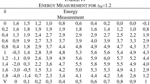
[image:4.595.288.551.50.184.2] [image:4.595.46.291.96.297.2]

(5)

The system's energy density is in the range of 0.4≤V≤1 and 0.6≤δ≤1.8, which is seen as in Fig. 5 and Table IV. The system's energy density varies between 4 and 5 energy units around these points.

TABLEIV

δ Energy

Measurement

0 1,6 1,5 1,2 1,0 0,8 0,6 0,4 0,2 0,0 0,0 -0,1 0,2 1,6 1,8 1,9 1,9 1,9 1,8 1,6 1,4 1,2 1,0 0,8 0,4 1,3 1,9 2,4 2,7 2,9 2,9 2,9 2,7 2,5 2,2 1,9 0,6 0,9 1,9 2,7 3,3 3,7 3,9 4,0 3,9 3,7 3,3 2,9 0,8 0,4 1,8 2,9 3,7 4,4 4,8 4,9 4,9 4,7 4,3 3,7 1 -0,3 1,4 2,8 3,9 4,8 5,3 5,6 5,6 5,4 4,9 4,3 1,2 -1,1 0,9 2,6 3,9 4,9 5,6 5,9 6,0 5,7 5,2 4,4 1,4 -2,0 0,3 2,2 3,6 4,7 5,5 5,8 5,9 5,5 4,9 4,0 1,6 -3,0 -0,5 1,5 3,1 4,2 5,0 5,3 5,3 4,9 4,1 2,9 1,8 -4,0 -1,4 0,7 2,3 3,4 4,1 4,4 4,2 3,6 2,6 1,2 V 0 0,1 0,2 0,3 0,4 0,5 0,6 0,7 0,8 0,9 1

For δm=1.2 rad. and w=1 p.u., Table IV shows numerical

) 209 . 0 cos( 4 ) 687 . 1 cos( ) 209 . 0 sin( 3 . 0

)... 687 . 1 sin( 075 . 0 907 . 14 426 . 2 a₂

 

   

 

 

 



 

(34)

) 209 . 0 sin( 20 ) 687 . 1 sin( 5

)... 513 . 1 cos( 5 ) 213 . 0 cos( 5 8 . 2 140 . 5 a1

 

 

 

 

 



(35)

) 209 . 0 cos( 386 . 3 ) 687 . 1 cos( 846 . 0

)... 209 . 0 sin( 254 . 0 ) 687 . 1 sin( 063 . 0 3 . 1 241 . 2 a

 

 

  

 



(36)

The system's energy density is in the range of 0.3≤V≤1 and 0.4≤δ≤1.6, which is seen as in Fig. 6 and Table V. The system's energy density varies between 3 and 4 energy units around these points.

TABLEV

δ Energy

Measurement

0 1,1 1,1 1,2 1,2 1,2 1,3 1,3 1,4 1,6 1,8 2,1 0,2 1,0 1,4 1,7 1,9 2,1 2,2 2,3 2,3 2,4 2,4 2,4 0,4 0,8 1,5 2,1 2,6 2,9 3,1 3,2 3,2 3,2 3,1 2,9 0,6 0,5 1,5 2,4 3,0 3,5 3,8 4,0 4,0 3,9 3,6 3,3 0,8 0,0 1,3 2,5 3,3 4,0 4,4 4,6 4,6 4,4 4,1 3,5 1 -0,6 1,0 2,4 3,4 4,2 4,7 4,9 4,9 4,7 4,2 3,5 1,2 -1,4 0,5 2,1 3,3 4,2 4,7 5,0 4,9 4,6 3,9 3,1 1,4 -2,2 -0,1 1,6 2,9 3,9 4,4 4,6 4,5 4,0 3,3 2,2 1,6 -3,1 -0,9 0,9 2,3 3,3 3,8 3,9 3,7 3,1 2,1 0,7 1,8 -4,1 -1,7 0,1 1,5 2,4 2,8 2,8 2,4 1,6 0,3 -1,3 V 0 0,1 0,2 0,3 0,4 0,5 0,6 0,7 0,8 0,9 1

For δm=1.6 rad. and w=1 p.u., Table V shows numerical

After all of these cases, we observed that the value of the whole energy density decreased. This decrease in energy measurement is an indicator of operating point’s movement towards instability region. In case-1, while δ=1.2 rad. and V=0.8 p.u., maximum energy level was 9.1 energy unit. But in case-5, energy level was 4.6 energy unit even the same value of δ and V. It is observed clearly that, any changes in load is going to continue decrease level of energy density to low values, even possible to see negative values.

V. CONCLUSION

Energy function has long been recognized as a useful way of analysing voltage stability. Our study shows that a more realistic energy function -which can clearly demonstrate the critical load angles gained on the energy measurement levels, corresponding to the representations of system works in the different levels and load voltages, and a single-machine infinite-bus power system’s stability attitude- can be obtained. Thus, this shows the effect of energy fluctuations in the system on system stability, nearly definitely. Eventually, for the system dependency to load angle and load voltage, optimal range of load angle and load voltage can be defined with the energy fluctuation which is plotted the range of stability shown.

APPENDIX

The load parameter values used in the simulation are [15]: Kpw = 0.4, Kpv = 0.3, Kqw = -0.03, Kqv = -2.8, Kqv2 = 2.1

T = 8.5, P0 = 0.6, Q0 = 1.3, P1 = 0.0, Q1 = 0.0

The network and generator parameter values used in the simulation are [15]:

Y0 = 20, θ0 = -5, E0 = 1, C = 12, Y0' =8, θ0' = -12

E0' = 2.5, Ym = 5, θm = -5, Em = 1, Pm = 1, D = 0.05

M =0.3

All values are in per unit except for angles, which are in degrees.

REFERENCES

[1] C. P. Steinmetz, “Power control and stability of electric generating stations,” AIEE Transactions, Vol. XXXIX, Part II, pp. 1215–1287, July 1920.

[image:5.595.46.291.118.255.2]

(6)

[3] P. Kundur, Power System Stability and Control. Toronto: Mc Graw-Hill, Inc., 1994.

[4] IEEE Working Group on Voltage Stability, Voltage Stability of Power System: Concepts, Analytical Tools, and Industry Experience,

IEEE Special Publication. 90TH0358-PWR, 1990.

[5] T. Van Cutsem, “Voltage Instability: Phenomenon, Countermeasures and Analysis Methods,” Proc. IEEE, vol. 88, pp. 208–227, 2000. [6] D. J. Hill, “Nonlinear dynamic load models with recovery for voltage

stability studies,” IEEE Trans. Power Systems, vol. 8, pp. 166–176, February 1993.

[7] T. Van Cutsem, C. Vournas, Voltage Stability of Electric Power

Systems. Norwell, MA:Kluwer Academic Publishers, 1998.

[8] J. Viswanatha Rao, S. Sivanagaraju, “Voltage regulator placement in radial distribution system using discrete particle swarm optimization,” International Review of Electrical Engineering

(IREE), Vol. 3, No.3,pp. 525–531, 2008.

[9] M. Z. El-Sadek, “Preventive measures for voltage collapses and voltage failures in the Egyptian power system,” Electric Power

Systems Research, 44:203–211, 1998.

[10] L. S. Vargas, C. A. Canizares, “Time dependence of controls to avoid voltage collapse,” IEEE Trans. Power Systems, paper no.PE-006PRS, July 2000.

[11] Interim Report: Causes of the august 14th blackout in The United States and Canada, Tech. Rep., November 2003.

[12] US-Canada Power Systems Outage Task Force, First Report on the August 14 2003, Blackout in the United States and Canada: Causes and Recommendations, April 2004.

[13] J. J. E. Slotine, W. Li, Applied Nonlinear Control. New Jersey: Prentice-Hall, Inc., 1991, pp. 57–97.

[14] E. R. Scheinerman, Invitation to Dynamical Systems. Prentice Hall College, 2000.

[15] I. Dobson, H. D. Chiang, J. S. Thorp, L. Fekih-Ahmed, “A model of voltage collapse in electric power systems,” IEEE Proceedings of the

27th Conference on Decision and Control, Austin, Texas, December,

1988, pp. 2104–2109.

[16] H. D. Chiang, I. Dobson, R. J. Thomas, J. S. Thorp, L. Fekih-Ahmed, “On voltage collapse in electric power systems,” IEEE Transactions

on Power Systems, vol. 5, No. 2, pp. 601–611, May 1990.