Abstract—A large attention has been focused on the dynamic fault tree (DFT). Cut sequence is an algebraic approach to overcome the shortcomings of the traditional methods for DFT analysis. In the generation of cut sequences, temporal rules play a key role, and the complete temporal laws ensure any form of the DFT can be reduced to cut sequences. Recently, lots of temporal rules have been put forward, but none of them are proven to be complete. This paper provides concise, but complete temporal rules. At first, the algebraic framework for temporal rules was built. Secondly, we put forward seven temporal rules, which are proven to be valid. Then, binary-tree-based completeness validations for temporal rules were given. Finally, application demonstrates the efficiency of the proposed temporal rules. Complete temporal rules promote the establishment of an intact theoretical foundation for cut sequence approach.
Index Terms—reliability, dynamic fault tree, cut sequence, temporal rules, completeness
I. INTRODUCTION
ault tree model is well accepted by reliability engineers and researchers for its advantages of compact structure and integrated analyzing methods. While traditional (static) fault trees cannot deal with the systems that characterize dynamic behaviors, such as sequential failure or redundancy. In the past few years, a large attention has been focused on the dynamic fault tree (DFT) [1]. By adding new gates to static fault tree, DFT aims to take into account dependencies among events (which typically exist in systems with spare components).
Markov chains (MCs) and their extensions have proven to be a versatile tool for analyzing the DFT [1] [2]. However, the MC-based approaches are faced with two well-known problems: (1) ineffectiveness in solving large dynamic models, i.e. the number of states grows exponentially as the number of the basic events in the system increases; (2) lack of modeling power capabilities, i.e. the failure time distribution is limited to the exponential distribution.
Manuscript received Dec. 10, 2012. This work was supported in part by the National Natural Science Foundation of China under Grant 60904082.
Li Yi is with the Academy of Equipment, Beijing 101416, China (e-mail: [email protected]).
Wang Bo is with the China Astronaut Research and Training Center, Beijing 100094, China (phone: 86-13701103586; fax: 86-10-66364116; e-mail: [email protected]).
Liu Dong is with the Academy of Equipment, Beijing, 101416 China (e-mail: [email protected]).
Yang Haitao is with the Academy of Equipment, Beijing, 101416 China (e-mail: [email protected]).
Yang Fande is with the Academy of Equipment, Beijing, 101416 China (e-mail: [email protected]).
The difficulty in (1) mainly comes from the existence of repeated events. A repeated event is defined as an event connected to several gates. To overcome the problem of (1), some researchers proposed methods to reduce the size of the MC by a modularization technique [3]. Static modules are analyzed by a binary decision diagram-based algorithm, and MCs are applied to the dynamic modules. However, in many cases, the size of a single module remains significant, and potentially leads to an unreasonable long computation times. Hence, the applicability of the modularization technique is not always evident.
As a method to extend the modeling capability, i.e., as an alternative method to deal with the problem of (2), the algebraic approach of the DFT has been proposed. Liu et al. [4] proposed a method of DFT analysis called CSSA (Cut Sequence Set Algorithm). In CSSA, the DFT is reduced into a set of cut sequences called sequential failure expressions (SFEs), which are ordered lists of events connected by the sequential failure symbol. The CSS (Cut Sequence Set) is the collection of all SFEs that represent the fault tree. Therefore, the CSSA method avoids the use of MCs entirely. Another algebraic approach is proposed by Merle et al [5], they put forward the complete algebraic expression of the DFT via introducing new temporal operators in order to define the sequence dependence of the gates. By using the operators and the conventional Boolean operators, the occurrence time of a top event (TE) is represented as a sum of the product canonical form. The terms of this form correspond to the minimal cut sequence set of the DFT.
Algebraic analysis of static fault trees consists of reducing any form of fault tree to its cut sets, which relies on a set of complete Boolean rules to function. In the generation of cut sequence of the DFT, Boolean rules are not sufficient for the DFT analysis. Therefore, more logical rules are needed, and we can apply to these temporal gates. These rules are named temporal rules. Complete temporal rules ensure any form of the DFT can be reduced to cut sequences. In Liu and Merle’s works, lots of temporal rules have been put forward, unfortunately, none of them told us their rules are complete.
In this paper, we propose novel and concise temporal rules for generating cut sequences. In order to prove the temporal rules are complete, we firstly build up a rigorous algebraic framework for temporal rules, then we seek for the common form of algebraic expressions for the DFT, finally the temporal rules’ completeness proof is given.
II. BACKGROUND A. Dynamic Fault Trees
Static fault tree (SFT), only captures the combination of
Complete Temporal Rules for Cut Sequence
Generation in Dynamic Fault Tree Analysis
Li Yi, Wang Bo, Liu Dong, Yang Haitao, Yang Fande
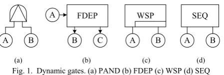
events, and is inadequate to model today’s complex dynamic systems. DFT analysis is an extension of SFT analysis that allows the modeling of dynamic behavior (sequence of events and functional dependence between events). DFT takes into account not only the combination of failure events but also the order in which they occur. DFT defines special gates that capture a variety of failure sequence and functional dependence. The six dynamic gates are proposed; the priority AND (PAND) gate, the functional dependency (FDEP) gate, the hot spare (HSP) gate, the warm spare (WSP) gate, the cold spare (CSP) gate and the sequence enforcing (SEQ) gate. The PAND gate is used to represent the dependence of the event sequence. It is logically equivalent to an AND gate, for which input events must occur in a specific order for the output event to occur. The output of a PAND gate with two inputs depicted in fig. 1 (a) becomes true if and only if both events A and B have occurred and event A has occurred before event B. The FDEP gate in fig. 1 (b) has a single trigger input A, and one or more dependent basic events. The dependent events are functionally dependent on the trigger event. When the trigger event occurs, the dependent events B is forced to occur. The WSP gate generalizes the CSP gate and the HSP gate. Fig. 1 (c) shows a WSP gate with two warm spares. The event A is a primary input that is originally powered on, and the other inputs specify the components that are used as replacements for the primary unit. The failure rates of spare units are reduced by a factor α, called the dormancy factor in standby mode. If α = 0, the gate is a CSP gate. And if α = 1, it is regarded as an HSP gate. The WSP gate has one output that becomes true after all the input events occur. The SEQ gate in fig. 1 (d) forces events to occur in a particular order. The input events are constrained to occur in the left-to-right order. However, it was shown in [6] that the SEQ gate is expressible in terms of the CSP. As a consequence, dynamic gates can be limited to gates PAND, FDEP, and Spare, only.
FDEP WSP SEQ
A B A
B C A B A B
[image:2.595.57.282.502.577.2](a) (b) (c) (d)
Fig. 1. Dynamic gates. (a) PAND (b) FDEP (c) WSP (d) SEQ
B. Cut Sequence
The occurrence of the DFT’s TE depends not only the combinations of basic events, but also the basic events’ sequential failure, called cut sequence, and the set of cut sequence is accordingly named cut sequence set (CSS). The CSS depicts components’ dynamic behaviors causing the system’s failure, which is the focus and difficulty in the DFT’s research.
In Liu’s CSSA approach, X→Y is a SFE in which X fails first and then Y fails. AND gates are converted into SFEs by enumerating all possible sequences, of which there are n! for a gate with n inputs; thus an AND gate with three inputs, e.g. X.Y.Z, would yield 6 SFEs: X→Y→Z, X→Z→Y, Y→X→Z, Y→Z→X, Z→Y→X, and Z→X→Y. PAND gates indicate a single SFE directly, e.g. X PAND Y is the same as X→Y.
FDEP gates are represented as (E1 AND E2) OR E3, where E1, E2, and E3 are SFEs representing the trigger event, the triggered events, and any non-triggered events respectively. Finally, SPARE gates (WSP, CSP and HSP) are represented by specific SFEs that link the failure of the primary to the failure of the secondary.
III. TEMPORAL RULES’ALGEBRAIC FRAMEWORK A. Non-repairable Events
The events of DFT are considered as non-repairable in this paper. It is also assumed that events occur instantaneously. To count on the temporal aspect of events, in accordance with Merle’s work, we consider events are piecewise right continuous on R+ ∪ {+∞}. Each of them is defined by its unique time of occurrence, noted t (A) for an event A. In this paper, we denote by BE the set of non-repairable events.
For any v BE, an assignment over v is any mapping from v to {0, 1}. Assignments are extended inductively into mappings from Boolean formulae into {0, 1}. Let σ be an assignment, then
1 ( )
0 ( )
otherwise v
if t v
And
( ) 1 ( ) 0 ( ) 0 ( )
I if t I
if t
B. Operators
Any elements of BE can be composed thanks to a rewriting of classical Boolean operators. The temporal definition of Boolean operators OR (+) and AND (·), based on the assignments of a and b is
( ) max{ ( ), ( )} ( ) min{ ( ), ( )}
a b a b
a b a b
To model the sequence of occurrence of events, we introduce an operator PRIORITY (with symbol ≺), whose formal definition, based on the assignments of a and b, is (with a given time interval [0, T] )
1 0 ( ) ( )
( )
0 t a t b T a b
otherwise
It can be seen that the order of inputs to AND and OR gates is irrelevant. However, the dynamic gates, such as PAND, SPARE, and SEQ, depend on the order of their inputs. The PRIORITY is not a commutative operator.
C. Behavior Model of Static and Dynamic Gates under the Framework
This chapter presents the behavioral model of dynamic gates which has been built thanks to the 3 operators in order to determine the structure function of the DFT. The behavioral model of gates OR, AND, PAND, FDEP, and Spare is presented as follows.
1) OR and AND gate
occurs, assume its inputs events are A and B, a behavioral model of OR gate can hence be determined as
A + B
For the AND gate, if all of its inputs events occur, its output event occur, so the behavioral model AND gate with inputs events A and B is
A · B 2) PAND gate
The PAND gate is a special case of the AND gate in which the output event occurs only if all input events occur in a specified ordered sequence. A behavioral model of PAND gate in fig. 1(a) can be modeled as
A ≺ B 3) FDEP gate
The FDEP gate is a dynamic gate, but its behavioral model is equivalent to a static model, which has been demonstrated in many references. The behavioral model in fig. 1(b) is
B + A B + C
4) WSP gate
The behavioral model of Spare gates will be presented in an increasing order of complexity. Let us consider a Spare gate with 2 input events, the primary event A and one spare event B, as shown in fig. 1(c). As stated in [7], the output event of the gate occurs when the primary and all spares have failed, so when A and B have failed If A and B fail according to sequences A≺B or B≺A. It is important to note that in sequence A≺B, B fails while in its active mode (denoted as Ba), whereas in sequence B≺A, B fails while in its dormant mode (denoted as Bd) [5]. The behavioral model of the WSP gate can be determined as
A≺Ba + Bd≺A
For the CSP gate, because B can only fail in its active mode, the behavioral model is
A≺Ba A simper form is
A≺B
Some more complicated behavioral models in detail can be found in [5][8].
IV. PROPOSED TEMPORAL RULES
Operators OR, AND and BEFORE satisfy the following temporal rules, for all a, b, c BE:
Rule 1 (R1). (a≺b)≺c a≺b≺c
Rule 2 (R2). a≺(b≺c) a≺b≺c + b≺a≺c Rule 3 (R3). a≺(b+c) a≺b + a≺c Rule 4 (R4). (a+b)≺c a≺c + b≺c Rule 5 (R5). a≺a a
Rule 6 (R6). a≺b≺a ∅ Rule 7 (R7). a·b a≺b + b≺a
The symbol “” means it can be reduced from left to right, and right to left in the rule expression, while “” indicates that it can be only reduced from left to right, hence,
we cannot say that a≺b + a≺c a≺(b+c) , which is not a valid rule.
The validities of the proposed temporal rules can be mathematically proved with the aid of temporal rules’ algebraic framework. If assignments of both sides of the rule are the same value, we reckon that the rule is valid. We will take Rule 1 for example.
Proof of Rule 1(R1): (a≺b)≺c a≺b≺c
For this proof, we will firstly add the following definition: 1 0 ( ) ( ) ( )
( )
0
t a t b t c T a b c
otherwise
1. Case 1: If any one of t(a), t(b), t(c) is not in time interval [0, T], by definition, the assignment of the left side of R1 is 0, so as the right side of R1. Hence, the assignment of the left side equals the right side of R1 in case 1, the following we consider all of t(a), t(b), t(c) are in time interval [0, T].
2. Case 2: 0≤t(a)≤t(b)≤t(c)≤T. By definition, σ(a≺b≺c) = 1, t(a≺b) = t(b), t(a≺b) ≤ t(c), σ((a≺b)≺c) = 1, so the assignments of both sides of R1 is 1.
3. Case 3: 0≤t(a)≤t(c)≤t(b)≤T. By definition, t(a≺b) = t(b) , then t(c) ≤ t(a≺b), so σ((a≺b)≺c) = 0, and σ(a≺b≺c) = 0. The assignments of both sides of R1 is 0.
4. For other cases, such as 0≤t(b)≤t(a)≤t(c)≤T, 0≤t(b)≤t(c)≤t(a)≤T, 0≤t(c)≤t(a)≤t(b)≤T, 0≤t(c)≤t(b)≤t(a)≤T, it can be easily validated by definition that the assignments of both sides of R1 is 0.
In conclusion, the assignments of both sides of R1 in any cases are the same.
End of the proof of R1.
V. COMPLETENESS VALIDATIONS FOR TEMPORAL RULES A. Irreducible Element: Disjunctive Priority Normal Form
The completeness of temporal rules is to constructing a rules’ system that can deduce all formulae into irreducible forms, called disjunctive normal forms, which is the key point of theoretical foundation for generation of cut sequences. It can guarantee any forms of the DFT deduced into cut sequence form. Take a broad view of the current study, research results within this respect are not published.
To solve this problem, we need firstly establish the judgment standard of completeness, the starting point lies in the definition of irreducible element in cut sequences. We extend the traditional disjunctive normal form with temporal factors, define:
Def. 1 PNF (Priority Normal Form) Variables in the
formulae are connected only by operator PRIORITY.
Def. 2 DPNF (Disjunctive PNF) All priority normal
forms are connected only by operator OR.
The PNF and DPNF are cut sequence and cut sequence set respectively.
B. Binary-tree-based Common Form of Formulae
Binary tree is an ordered tree that contains at most two sub trees for each node. Operators in this paper are all dualistic, so we can translate formulae into the binary tree form. The root node of a binary tree is the last operation symbol. We stipulate the operation order as (from high to low):
·, ≺,
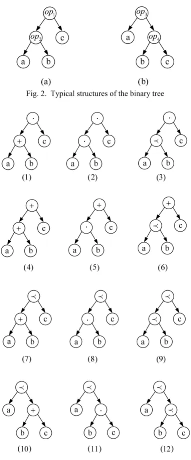
Typical structures of the binary tree are shown in fig. 2, where op1, …, op4 represent operators between nodes. For that operators OR(+) and AND (·) are commutative, if op1, op3 ∈ {·, +}, fig. 2(a) is equivalent to fig. 2(b), which means a same type of formulae. Operator PRIORITY is not commutative, so if op1, op3 ∈ {≺}, fig. 2(a) is different from fig. 2(b).
2
op
1
op
4
op
3
[image:4.595.73.265.233.695.2]op
Fig. 2. Typical structures of the binary tree
Fig. 3. Binary Trees that representing all formulae
Hence, if op1 {·, }, then op2 {·, ≺, }; if op1 {≺}, then op2 {·, ≺, ,}; if op3 {≺}, then op4 {·, ≺, }. Finally, we obtain 12 (= 6 + 3 + 3) binary trees, as shown in fig. 3. It can be easily checked that there are not repeated and isomorphic trees among those 12 trees.
C. Completeness Validation
1) Convert binary trees to formulae
Firstly, we need to obtain the algebraic expressions of 12 binary trees, and it can be handled out with in-order-traversal strategy, the main process is:
1. Visit left sub-tree, if the root node is not a leaf, and its operation order is posterior to its father node’s, then add a left parentheses before visiting, and add a right parentheses at the end of visiting.
2. Visit right sub-tree, if the root node is not a leaf, and its operation order is posterior to its father node’s, then add a left parentheses before visiting, and add a right parentheses at the end of visiting.
3. Visit any sub-trees, if the root node is not a leaf, and the connection symbols of root node and father node are all PRIORITY, then add a left parentheses before visiting, and add a right parentheses at the end of visiting.
According to this process, we obtain the algebraic expressions, as listed in TABLE I.
TABLEI
ALGEBRAIC EXPRESSIONS OF BINARY TREES
No. Expression
(1) (a+b)·c (2) a·b·c (3) (a≺b)·c (4) a+b+c (5) a·b+c (6) a≺b+c (7) (a+b) ≺c (8) a·b≺c (9) (a≺b) ≺c (10) a≺ (b+c) (11) a≺b·c (12) a≺(b≺c)
If the proposed temporal rules are complete, then any algebraic expressions in TABLE I can be deduced to DPNF. We check those expressions one by one, and the results are shown in TABLE II.
Typically, we chose (11) to demonstrate the deduction process.
To deduct: a≺b•c
a≺b≺c+b≺a≺c+a≺c≺b+c≺a≺b.If b=c, a=c, b=a, and b=a=c, it can be easily verified. We consider a ≠ b ≠ c.
Employing R7, R3 and R2, we have:
a≺b•c
a≺(b≺c+c≺b)
a≺(b≺c)+ a≺(c≺b)
a≺b≺c + b≺a≺c + a≺c≺b + c≺a≺b .End of the deduction.
TABLEII
DEDUCTION RESULTS OF ALGEBRAIC EXPRESSIONS
No. Result DPNF? Rules Used
(1) a≺c+c≺a+b≺c+c≺b Y BRs (2) a≺b≺c+a≺c≺b+b≺a≺c+b≺c≺a+c≺a≺b+c≺b≺a Y BRs,
R1, R2, R7 (3) a≺b≺c+c≺a≺b+a≺c≺b Y R1,
R2, R7 (4) dispense with deduction Y NONE
(5) a≺b+b≺a+c Y R7
(6) dispense with deduction Y NONE
(7) a≺c+b≺c Y R4
(8) a≺b≺c+b≺a≺c Y R4, R7
(9) a≺b≺c Y R1
(10) a≺b+a≺c Y R8
(11) a≺b≺c+b≺a≺c+a≺c≺b+c≺a≺b Y BRs, R2, R3, R7 (12) a≺b≺c+b≺a≺c Y R2
Y= the result is a DPNF, BRs = Boolean Rules, R = rule
VI. APPLICATIONS
The Cardiac Assist System (CAS) [9] is designed to treat mechanical and electrical failures of the heart. The system can be divided into 4 modules: Trigger, CPU unit, motor section, and pumps. In this paper, we focus on the pumps unit.
[image:5.595.309.537.64.410.2]The pumps unit is comprised of two cold spares, each having a primary pump (PUMP_1 and PUMP_2), and sharing a common spare pump (Backup_PUMP). In order for the pumps unit to fail, all three pumps need to fail and CSP_1 needs to fail before (or at the same time as) CSP_2. The DFT which models the potential failure of the pumps unit of CAS is shown in Fig. 4
Fig. 4. The DFT of pumps unit of CAS
The behavioral model of PAND gate presented in Section III allows expressing PUMPS as
PMMPS = CSP1 ≺ CSP2 According to the behavioral model of Spare gate
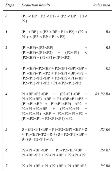
CSP1 = P1 ≺ BP + P2 ≺ P1 CSP2 = P2 ≺ BP + P1≺ P2 CSP1 ≺ CSP2 can now be expressed as
Steps Deduction Results Rules used 0 (P1 ≺ BP + P2 ≺ P1) ≺ (P2 ≺ BP + P1≺
P2)
1 (P1 ≺ BP ) ≺ (P2 ≺ BP + P1≺ P2) + (P2 ≺ P1 ) ≺ (P2 ≺ BP + P1≺ P2)
R4
2 (P1≺BP)≺(P2≺BP) + (P1≺BP)≺(P1≺P2) + (P2≺P1) ≺
(P2≺BP) + (P2≺P1)≺(P1≺P2)
R3
3 (P1≺BP)≺P2≺BP + P2≺(P1≺BP)≺BP + (P1≺BP)≺P1≺P2 + P1≺(P1≺BP)≺P2 + (P2≺P1)≺P2≺BP + P2≺(P2≺P1)≺BP + (P2≺P1)≺P1≺P2 + P1≺(P2≺P1)≺P2
R2
4 P1≺BP≺P2≺BP + (P2≺P1≺BP +
P1≺P2≺BP) ≺BP + P1≺BP≺P1≺P2 + (P1≺P1≺BP + P1≺P1≺BP) ≺P2 + P2≺P1≺P2≺BP + (P2≺P2≺P1 + P2≺P2≺P1) ≺BP + P2≺P2≺P1≺P2 + (P1≺P2≺P1 + P2≺P1≺P1) ≺P2
R1 R2 R4
5 ∅ + (P2≺P1≺BP + P1≺P2≺BP) ≺BP + ∅ + (P1≺BP)≺P2 + ∅ + (∅ + P2≺P1)≺BP + ∅+ (∅+ P2≺P1)≺P2
R5 R6
6 P2≺P1≺BP≺BP + P1≺P2≺BP≺BP + P1≺BP≺P2 + P2≺P1≺BP + P2≺P1≺P2
R4 R1
7 P2≺P1≺BP + P1≺P2≺BP + P1≺BP≺P2 R5 R6 From algebraic view, in the deducting, we make use of R3, R3 is not a rigorous, equivalent rule (it can be only utilized from left to right), and it will bring conflicts in logic. Therefore, a check should be manipulated, which recurs to a physical meanings’ validation. From the real meanings, if P1 fails at first, BP will be used, and then if P2 fails secondly, there is no spares left, so output of CSP2 will occur, after BP fails, output of CSP1 occurs after CSP2, and the output of PUMPS won’t occur, which is not coincident with the physical meanings. Hence P1≺P2≺BP should be canceled. Finally, with application of the proposed temporal rules, we obtain two cut sequences
P2≺P1≺BP, P1≺BP≺P2
For instance, the algebraic term P2≺P1≺BP indicates that P2, P1 and BP must fail in this order, which is a dynamic failure mode.
VII. CONCLUSION
Temporal rules are key theoretic foundation in generating cut sequences in DFT analysis. This paper put forward several novel temporal rules, rigorous proofs and case’s application demonstrate the proposed temporal rules are valid and complete. In the future, we will resolve algorithms that would allow to automatically extract the cut sequences from the DFT.
REFERENCES
[1] J. B. Dugan, S. J. Bavuso, and M. A. Boyd, “Dynamic fault tree models for fault-tolerant computer systems,” IEEE Trans. on Reliability, vol. 3, 1992, pp. 363–377.
[2] H. Boudali, P. Crouzen, M. Stoelinga, “A compositional semantics for dynamic fault trees in terms of interactive Markov chains”, In: Proceedings of the international symposium on automated technology for verification and analysis (ATVA’07), Springer Verlag — LNCS, vol.4762;2007. p.441–56.
[3] R. Gulati, J. B. Dugan, “A modular approach for analyzing static and dynamic fault trees”, Proceedings of Annual Reliability & Maintainability Symposium, Philadelphia, PA1997:568–73.
[4] L. Dong, X. Weiyan, Z. Chunyuan, L. Ri, and H. Li, “Cut Sequence Set Generation for Fault Tree Analysis”, Proc. Of International Conference on Embedded Software and Systems. Daegu,South Korea, 14-16 May 2007,LNCS 4523,pp.58-69
[5] G. Merle ,“Algebraic modeling of Dynamic Fault Trees, contribution to qualitative and quantitative analysis”, PhDthesis, LURPA, ENS de Cachan; July 2010
[6] H. Boudali, P. Crouzen and M. Stoelinga ,“Dynamic Fault Tree analysis through input/output interactive Markov chains,” In Proceedings of the International Conference on Dependable Systems and Networks (DSN 2007), pages 25–38, Edinburgh, UK, 2007 [7] M. Stamatelatos and W. Vesely , “Fault Tree Handbook with
Aerospace Applications”, NASA Office of Safety and Mission Assurance, vol. 1.1, pages 1–205, 2002.
[8] B. Wang, D. Liu, and Y. Li, “Algebraic Modeling for Dynamic Gates in Dynamic Fault Trees,” International Conference on Mechanical and Aerospace Engineering (ICMAE 2012), July 7-8, 2012, Paris, France, pp. 573-577