Assessing horizontal accuracy of inventory plots in forests with different mix of tree species composition and development stage

JOURNAL OF FOREST SCIENCE, 64, 2018 (11): 478–485

https://doi.org/10.17221/92/2018-JFS

Assessing horizontal accuracy of inventory plots

in forests with different mix of tree species composition

and development stage

Vlastimil MURGAŠ

_{*, Ivan SAČKOV}

_{, Maroš SEDLIAK}

_{, Daniel TUNÁK}

_,

František CHUDÝ

1_{National Forest Centre – Forest Research Institute Zvolen, Zvolen, Slovak Republic}

2 _{Department of Forest Management and Geodesy, Faculty of Forestry,}

Technical University in Zvolen, Zvolen, Slovak Republic *Corresponding author: [email protected]

Abstract

Murgaš V., Sačkov I., Sedliak M., Tunák D., Chudý F. (2018): Assessing horizontal accuracy of inventory plots in forests with different mix of tree species composition and development stage. J. For. Sci., 64: 478–485. Global navigation satellite systems (GNSS) have a wide range of applications in forest industry, including forest inven-tory. In this study, the horizontal accuracy of 45 inventory plots in different forest environments and 5 inventory plots under open sky conditions were examined. The inventory plots were located using a mapping-grade GNSS receiver during leaf-on season in 2017. True coordinates of the plot centres were acquired using a survey-grade GNSS receiver during leaf-off season in 2018. A study was conducted across a range of forest conditions in the forest unit Vígľaš, which is located in Slovakia (Central Europe). Root mean square error of horizontal accuracies was 8.45 m in the plots under forest canopy and 6.61 m under open sky conditions. We note decreased positional errors in coniferous forests as well as in younger forests. However, results showed that there is no statistically significant effect of tree species composition and stand age on horizontal accuracy.

Keywords: GNSS; positional error; satellite navigation; spatial coordinates

Global navigation satellite system (GNSS) is the generic term for satellite navigation systems that provide autonomous geo-spatial positioning with global coverage. Current fully-operational GNSS include the United States Global Positioning Sys-tem (GPS) and the Russian Globalnaja Navigat-sionnaja Sputnikovaja Sistema (GLONASS). The European Union and China are developing their own satellite-based systems Galileo and BeiDou-2/ Compass, respectively (Xu, Xu 2016).

In recent decades, there has been growing in-terest for GNSS applications in forestry because obtaining spatial data can be performed rapidly,

efficiently and accurately. Typical GNSS-based ap-plication includes plot establishment for forest in-ventory or environmental monitoring (Johnson, Barton 2004; Awange 2012). Of the many vari-ables resulting from forest inventory, plot position is yet essential. The reason is that accurate infor-mation regarding plot position (i) enables quick revisitation of the plot for subsequent remeasure-ment, (ii) provides relevant spatial information for mapping, and (iii) is crucial for many analyses using remote sensing and GIS techniques. How-ever, only handheld recreational- or mapping-grade receivers are commonly used in establishing

and relocating inventory plots (Hoppus, Lister 2007). The declared horizontal accuracy of these receivers is within 6–10 m, but there has been no detailed or wider study revealing the explicit horizontal accuracy of inventory plots in different forest conditions.

It is common knowledge that tree canopies ad-versely affect the accuracy of GNSS positioning because they obstruct and reflect radio signals and deteriorate the receiver ability to fix location (D’Eon 1995; Deckert, Bolstad 1996; Hasega-wa, Yoshimura 2003). According to Sigrist et al. (1999), the presence of an overhead canopy may degrade the positional precision by one order of magnitude. Additional errors to GNSS observa-tions are introduced due to ionospheric effects, atmospheric effects, relativistic effects, clock er-rors, and other (Xu, Xu 2016). Weaver et al. (2015) found that there is significant influence of holding position of a GNSS receiver on static horizontal accuracy. Their results indicated that higher positional accuracies can be obtained if the GNSS receiver is held vertically. It has been dem-onstrated that raising the antenna height signifi-cantly enhances the positioning accuracy of GNSS measurements especially during the leaf-off sea-son (Brach, Zasada 2014). Nonetheless, placing an antenna in close proximity of tree crown and foliage results in decreased measurement accura-cy. As noted by Karsky (2004), there are several ways to correct GNSS acquired data. For example, it is possible to apply real-time corrections by us-ing differential GPS (DGPS) and the wide-area augmentation system (WAAS). However, the most accurate positioning information is derived using static method with longer observation times and requires post-processing.

Numerous studies have examined the perfor-mance of different GNSS receivers and position-ing methods under a variety of environmental conditions (e.g. Yoshimura, Hasegawa 2003; Bolstad et al. 2005; Piedallu, Gégout 2005; Rodríguez-Pérez et al. 2007; Wing et al. 2008; Bettinger, Fei 2010; Valbuena et al. 2010; Wing 2011; Tomaštík et al. 2016). As described in Wing et al. (2005), users equipped with rec-reational-grade GPS receivers could expect posi-tional accuracies within 5 m of true position in open sky conditions, 7 m in young forest condi-tions, and 10 m in closed canopies. Application of mapping-grade GPS receivers with real-time differential corrections would provide average measurement error smaller than 1 m in open area conditions as well as in young forests, and 2.2 m

under forest canopy (Wing et al. 2008). Tuček and Ligoš (2002) investigated positioning errors of three GPS receivers under the forest canopy during leaf-on season. They used multi-factor analysis of variance to assess the influence of re-ceiver type, stand age, tree species composition and terrain configuration. Their analysis showed significant influence of stand age and receiver type on positioning error. The effects of tree spe-cies composition and terrain configuration on po-sitioning errors were ambiguous. On the contrary, Bettinger and Fei (2010) found that positional error significantly differs in broadleaved, older pine, and young pine stands, regardless of season. The annual mean horizontal accuracy value was best in the older pine stand (6.6 m), second best in the broadleaved stand (7.9 m) and worst in the young pine plantation (11.9 m). Bettinger and Merry (2012) assessed the GPS accuracy with re-gard to spatial arrangement of nearby trees in a young loblolly pine (Pinus taeda Linnaeus) planta-tion. They concluded that the presence of live de-ciduous trees within the plantation may affect the static horizontal accuracy. Naesset et al. (2000) demonstrated that employing combined differen-tial GPS and GLONASS measurements resulted in increased positional accuracy in a mixed forest of spruce, pine and birch in Norway. Hasegawa and Yoshimura (2003) suggested the use of dual-fre-quency GPS receivers to acquire the most accurate positional data under tree canopies. Nonetheless, Valbuena et al. (2010) found no significant differ-ence between single- and dual-frequency receiv-ers. However, there has been little discussion on whether positional errors of established inventory plots were inside admissible boundaries needed for further data processing (Mauro et al. 2009; Kitahara et al. 2010; Zald et al. 2014). For ex-ample, Kitahara et al. (2010) examined the hori-zontal accuracy of national forest inventory plots in Japan. The total mean positional error and pre-cision were 8.6 and 12.6 m, respectively. When it comes to the tree species composition, lower val-ues of positional errors were found in broadleaved forests (5.6 m) and higher positional errors in co-niferous forest (9.6 m). Zald et al. (2014) showed that improved GPS plot locations had little impact on the accuracy of derived imputation maps.

for-ests, (ii) older forfor-ests, and (iii) forests with dense canopy cover.

MATERIAL AND METHODS

Study area. The study was conducted in the ter-ritory of the forest unit Vígľaš (Fig. 1) located in central Slovakia (approximately 48°32'N, 19°21'E). The total area is 12,472 ha and forests occupy 3,215 ha of this area. The elevation of the study area reaches 374–978 m a.s.l. Dominant species in the area include European beech (Fagus sylvatica Linnaeus), Sessile oak (Quercus petraea (von Mat-tuschka) Lieblein), and European hornbeam (Car-pinus betulus Linnaeus) with 65% coverage. The area of the remaining part is covered by conifers, such as European silver fir (Abies alba Miller) and Norway spruce (Picea abies Linnaeus).

Dataset from forest inventory. Forest inven-tory was carried out during the leaf-on season in 2017. A total number of 295 inventory plots were established into a systematic 250 m grid (Fig. 1). We used a Topcon FC-25A field controller (Topcon Corporation, Japan) embedded with a mapping-grade GNSS receiver (Topcon 2018a). Duration of the observing sessions was within 10 min.

Tech-nical specifications for the mapping-grade receiver are summarized in Table 1. Finally, centre of each plot was invisibly fixed by a steel tube.

Dataset from validation survey. For the pres-ent study, 45 of 295 invpres-entory plots were selected by post-stratification, which was focused on the creation of nine strata (five plots per stratum). The main criteria for stratification were tree spe-cies composition and mean DBH as a surrogate for stand age. At first, coniferous stratum (C, coni-fers ≥ 70%), broadleaved stratum (B, broadleaves ≥ 70%), and a mixed stratum (M, conifers or broad-leaves < 60%) was created. At second, each stratum was divided into three development stages of forest stand. Here, the limits of mean diameter < 20 cm (C1, B1, M1), 20–30 cm (C2, B2, M2), and > 30 cm (C3, B3, M3) were used. In addition, 5 of 295 inven-tory plots in open sky conditions were selected for comparison of horizontal accuracy.

The validation survey was performed for select-ed inventory plots during leaf-off season in 2018 (Fig. 1). We used a survey-grade GNSS receiver Topcon Hiper GGD (Topcon Positioning Systems, Inc., USA) (Topcon 2018b) to obtain true coordi-nates of the plot centre that had been already found by metal detector. Technical specifications for the survey-grade receiver are summarized in Table 2. The validation measurements were conducted us-ing static GNSS survey technique. The elevation mask and antenna height were set at 5° and 2 m, respectively. Duration of the observing sessions was about 25 min. Acquired data were post-processed in Topcon Tools processing software (Version 8.23, 2012). Subsequently, resulting positions were trans-formed into the Slovak national coordinate system S-JTSK (System of Trigonometric and Cadastral Network) using the official transformation service (https://zbgis.skgeodesy.sk/rts/sk/Transform).

Accuracy assessment. The differences (Δxi and

Δy_i) between coordinates derived from a survey-grade GNSS receiver (x_iR, y_iR) and target coordi-nates (x_iT, y_iT) of a systematic 250 m grid were com-puted using Eqs. 1 and 2:

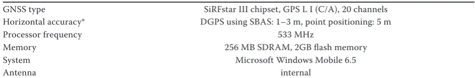
Table 1. Technical specifications for mapping-grade receiver Topcon FC-25A (Topcon Corporation, Japan)

GNSS type SiRFstar III chipset, GPS L I (C/A), 20 channels

Horizontal accuracy* DGPS using SBAS: 1–3 m, point positioning: 5 m

Processor frequency 533 MHz

Memory 256 MB SDRAM, 2GB flash memory

System Microsoft Windows Mobile 6.5

Antenna internal

*Accuracy depends on the number of satellites used, SBAS data quality, multipath objects, device position/posture and other environmental conditions

R T i i i x x x

   ₍₁₎

R T i i i y y y

   ₍₂₎

For each inventory plot position, the individual positional error (D_i) was calculated according to Eq. 3:

2 2

i i i

D    x y ₍₃₎

For each stratum, the mean positional error (D_), the standard error of the mean (SE), and the stan-dard deviation of positional error (SD) were calcu-lated using Eqs. 4–6:

1 n

i i D D

n





SD SE

n

 ₍₅₎





1

SD

1

n i i D D

n

 







Then we determined mean coordinate errors (RMSE) across all strata (n) according to Eqs. 7 and 8:

2 1

RMSE

n i i x

x n







2 1

RMSE

n i i y

y n







The root mean square coordinate error (RMSE_xy) of inventory plots as a measure of the horizontal accuracy depicts the deviation from the truth and was calculated by Eq. 9:

2 2

RMSExy RMSExRMSEy (9)

Shapiro-Wilk normality test was carried out at 95% confidence level in order to determine if the po-sitional errors (Δx_i and Δy_i) follow a normal distribu-tion. If the positional errors were normally distrib-uted, the parametric Student’s t-test was performed in order to validate the null hypothesis (Eqs. 10–13):

H₀: Δx̱ = 0 (10)

H₀: Δy̱ = 0 (11)

H₁: Δx̱ ≠ 0 (12)

H₁: Δy̱ ≠ 0 (13)

The null hypothesis states that the mean positional error is equal to zero, against the alternative hypoth-esis that it is not equal to zero. In the case of normal distribution of the positional error, the non-parametric Wilcoxon signed rank test was used.

To clarify the effect of tree species composition and stand age on horizontal accuracy, one-way ANOVA or Kruskal-Wallis H test was applied ac-cording to normal or non-normal distribution of positional errors, respectively. In the cases where ANOVA or Kruskal-Wallis H test proved signifi-cance of differences at the signifisignifi-cance level 0.05, mean values of positional errors were compared by Duncan’s multiple range test or Wilcoxon signed rank test, respectively. The statistical analysis was conducted in R software (Version 3.5.1, 2017).

RESULTS

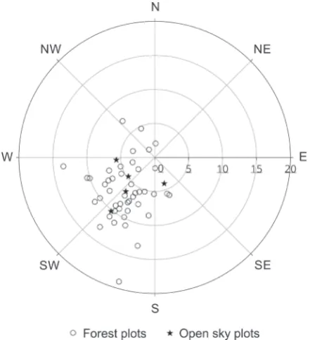
The individual positional errors D_i of validation inventory plots are shown in Fig. 2.

Analysing D_i for the 45 inventory plots under for-est canopy, it was observed that 16% of the errors were smaller than 5 m, 60% of the errors were with-in 5–10 m, and 24% of the errors exceeded 10 m. In addition, 55% of the errors angled south-west-wards, 20% of the errors angled southsouth-west-wards, 16% of the errors angled westwards, 7% of the errors angled north-westwards and only 2% of the errors angled northwards.

Results obtained from the 5 inventory plots un-der open sky conditions showed that 40% of D_i were under 5 and 10 m. But 20% of the errors were greater than 10 m. Again, when compared to the di-Table 2. Technical specifications for survey-grade receiver Topcon Hiper GGD (Topcon Positioning Systems, Inc., USA)

GNSS type GPS L1 + L2 + GLONASS (GGD), 40 channels

Horizontal accuracy static method: 3 mm ± 0.5 ppm; RTK: 10 mm ± 1.0 ppm

Recording frequency up to 20 Hz

Memory 96 MB

System Topcon’s PC-CDU software (Version 7.12, 2007)

Antenna microstrip

rection, 60% of the errors were angled west-wards and 20% of the errors were angled south-wards and westsouth-wards.

Descriptive statistics for individual positional er-rors (D_i) and horizontal accuracies (RMSE_xy) across all strata are illustrated in Table 3.

The minimum and maximum value of D_i for in-ventory plots under forest canopy was 1.42 and 19.00 m, respectively. The mean value of D_i was 7.72 ± 0.51 m. The variability of D_i ranged from 1.44 to 6.25 m. In total, 75.6% of the 45 inventory

plots had a value of D_i less than 10 m. The RMSE_xy for various combinations of tree species composi-tion and stand age varied from 6.11 to 10.31 m. Ac-cording to tree species composition, the RMSE_xy varied slightly between broadleaved (9.01 m) and mixed (9.1 m) stratum. However, lower value of 7.06 m was obtained for coniferous stratum. Thus, coniferous stratum was characterized by higher horizontal accuracy than the broadleaved and mixed stratum. Regarding stand age, lower values of RMSE_xy are characteristic for younger develop-ment stages of forests, except for stratum C2. The highest horizontal accuracy was found for stratum C1. On the contrary, the lowest horizontal accu-racy was found for stratum B3. The highest and lowest variability of D_i was found for stratum M2 and M3, respectively.

The minimum and maximum values of D_i for in-ventory plots under open sky conditions were 4.09 and 10.2 m, respectively. There, the mean value of D_i was 6.25 ± 1.07 m.

Results of the Shapiro-Wilk normality test are re-ported in Table 4. In most cases, the P-value is not less than the significance level of 0.05. Therefore, the tested errors along the x axes and the y axes are con-firmed to follow a normal distribution. The excep-tions are stratum B1 and M3 for errors along the x axes as well as stratum C2 for errors along the y axes.

The results of statistical tests (Table 5) confirmed that the errors along the x and y axes are biased in case of all forest plots and strata with different tree species composition (P < 0.05). This also shows Fig. 2 where a clear direction of D_i to the south-west is visible in both types of inventory plots under

for-Table 3. Horizontal accuracy (m) of inventory plots under forest canopy and open sky conditions

Stratum n D_ SE Minimum Maximum SD RMSE_xy

C 15 6.49 0.74 1.42 10.39 2.88 7.06

B 15 8.37 0.89 1.60 13.51 3.45 9.01

M 15 8.31 0.99 3.33 19.00 3.84 9.10

C1 5 5.59 1.24 1.42 9.11 2.78 6.11

C2 5 7.75 0.77 5.62 9.84 1.72 7.90

C3 5 6.13 1.75 2.05 10.39 3.91 7.06

B1 5 7.05 1.09 4.68 10.96 2.44 7.38

B2 5 8.71 1.34 5.23 13.02 2.99 9.11

B3 5 9.36 2.16 1.60 13.51 4.83 10.31

M1 5 7.22 1.19 3.34 10.88 2.67 7.61

M2 5 9.56 0.65 8.25 11.30 1.44 9.65

M3 5 8.15 2.79 3.33 19.00 6.25 9.88

Forest plots 45 7.72 0.51 1.42 19.00 3.45 8.45

Open sky plots 5 6.25 1.07 4.09 10.20 2.39 6.61

C – coniferous, B – broadleaved, M – mixed, n – sample number, D_ – mean positional error, SE – standard error of the mean, SD – standard deviation of positional error, RMSE_xy – root mean square coordinate error (horizontal accuracy) Fig. 2. Direction and magnitude of individual positional

est canopy and open sky conditions. Between strata depicting both tree species composition and stand age, however, the results are ambiguous. According to obtained results, only errors along the x axes are biased in open sky plots.

On the other hand, the one-way ANOVA showed no significant effect of tree species composition and stand age on positional error of inventory plots.

DISCUSSION

Our results demonstrated that the D_i and RMSE_xy varied greatly between inventory plots. Moreover, the difference between RMSE_xy for inventory plots under forest canopy (8.45 m) and RMSE_xy for plots under open sky conditions (6.61 m) was expected to be somewhat larger.

The largest and smallest positional error for a single position within plots under forest canopy was 19.00 and 1.42 m, respectively. In addition, the largest value of RMSE_xy was obtained in stratum B3 whereas the smallest value of RMSE_xy was obtained in stratum C1.

Unexpectedly, the minimum value of D_i within plots under open sky conditions was 4.09 m. We can assume that the satellite constellation was probably not optimal and the nearby forest edge caused deg-radation of satellite signal. Our argument is indirect-ly confirmed by Yoshimura and Hasegawa (2003) who found RMSE_xy at landing within the range of 2.42–6.67 m. Tuček and Ligoš (2002) tested three survey-grade GNSS receivers. They reported mean positional errors within the range of 1.96–7.50 m for open sky areas. Wing (2011) reported positional error of 1.5 m for the best performing consumer-grade GNSS receiver in the open sky course.

To examine the presence of bias in tested errors along the x and y axes Student’s t-test or Wilcoxon signed rank test were applied. Statistical analysis revealed that the systematic error was introduced into errors in case of all inventory plots under for-est canopy and strata with different tree species composition. This is a surprising result because we expected random direction of errors. The cause of biased errors can partly be attributed to the GNSS receiver and satellite errors. Our argument is based on the fact that approximately 8 inventory plots per day were established. On the other hand, we found no evidence of systematic error for few strata which represent combination of tree species composition and stand age. Biased error for open sky plots was only confirmed along the x axes.

Previous studies indicated that there is a signifi-cant difference between forest types, i.e. species composition or development stage (Bettinger, Fei 2010; Weaver et al. 2015). With respect to our study, we can conclude that there is no significant difference between mean positional errors across different forest strata. Although ANOVA did not prove significant effect of selected factors on posi-tional errors, we observed that the posiposi-tional errors more decreased in coniferous forests resulting in increased horizontal accuracy. Also, several studies Table 4. Results of the Shapiro-Wilk normality test

Stratum _W Δxi_{P-value W} Δyi_P-value

C 0.939 0.375 0.974 0.914

B 0.974 0.915 0.977 0.941

M 0.930 0.272 0.941 0.394

C1 0.784 0.059 0.919 0.524

C2 0.861 0.233 0.758 0.036

C3 0.832 0.145 0.914 0.490

B1 0.668 0.004 0.968 0.865

B2 0.826 0.131 0.829 0.137

B3 0.881 0.313 0.825 0.128

M1 0.890 0.358 0.922 0.541

M2 0.972 0.887 0.893 0.373

M3 0.773 0.048 0.938 0.650

Forest plots 0.971 0.324 0.987 0.898 Open sky plots 0.993 0.989 0.844 0.177 C – coniferous, B – broadleaved, M – mixed, Δx_i, Δy_i – dif-ferences between coordinates; significant P-values (< 0.05) are shown in bold

Table 5. Results of Student’s t-test or Wilcoxon signed rank test

Stratum Δxi Δyi

df P-value df P-value

C 14 0.007 14 < 0.000

B 14 < 0.000 14 0.001

M 14 < 0.000 14 < 0.000

C1 4 0.038 4 0.034

C2 4 0.229 – 0.125*

C3 4 0.202 4 0.053

B1 – 0.125* 4 0.154

B2 4 0.013 4 0.002

B3 4 0.043 4 0.154

M1 4 0.035 4 0.001

M2 4 0.001 4 < 0.000

M3 – 0.063* 4 0.024

Forest plots 44 < 0.000 44 < 0.000

Open sky plots 4 0.033 4 0.052

(Tuček, Ligoš 2002; Valbuena et al. 2010) did not confirm the influence of tree species composition on positioning errors. More pronounced degrada-tion of satellite signals in broadleaved forests has been previously noted (Wing 2011). Our results of positional errors in broadleaved and mixed strata were ambiguous. Nevertheless, positional errors tended to decrease in mixed strata compared to broadleaved strata. Controversially, horizontal ac-curacies were higher in broadleaved strata than in mixed strata. The results thus support the findings of Weaver et al. (2015). Bettinger and Merry (2012) noted that if the proportion of broadleaved trees at a radius of 4–5 m of a test point increased, the mean positional error increased. On the con-trary, Deckert and Bolstad (1996) reported in-creased positional errors in coniferous forests when compared to broadleaved forests. As noted by Weaver et al. (2015), this result could be attributed to differences in forest density and canopy cover. Horizontal accuracy was found to increase with de-creasing mean diameter in broadleaved and mixed forests. This finding is in line with previous studies. For example, Wing et al. (2005) showed that us-ers could expect horizontal accuracies within 7 m in young forest conditions and 10 m under closed canopies of older forest stands.

Overall, the horizontal accuracy of established inventory plots can be seen as satisfactory related to the used receiver, but this strongly depends on user’s preferences. Moreover, the DGPS may be considered a promising aspect of improved posi-tional accuracy. Therefore, forest managers decid-ing between GNSS receivers should choose one which supports DGPS corrections and allows con-necting an external antenna. For example, Wing et al. (2008) have reported smaller positional errors due to the use of external antennas when using GPS receivers in closed canopy sites.

CONCLUSIONS

This study examined the horizontal accuracy of 45 inventory plots established in different forest environments and 5 plots established in forests un-der open sky conditions.

The level of horizontal accuracy of mapping-grade receiver tested in this study, especially within plots under open sky conditions, was worse than expected. However, application of a mapping-grade GNSS receiver is still suitable for common estab-lishing inventory plots; if there is no emphasis on high positional accuracy (< 1 m).

We observed that RMSE_xy decreased in conifer-ous forests and younger forest stands. In this re-spect, we may conclude that admixture of broad-leaved trees and higher stand age adversely affect horizontal accuracy. However, our results indicated that effect of tree species composition and develop-ment stage on horizontal accuracy is not statisti-cally significant.

The ongoing modernization and expansion of GNSS will offer much improved horizontal accu-racy, integrity and efficiency performances for dif-ferent specific areas over the world. In this context, GNSS-based forestry applications are expected to be on the uptrend. Consequently, continuous ac-curacy assessment of GNSS receivers seems to be valid and necessary (Bettinger, Fei 2010). This is an issue for future research to explore.

References

Awange J.L. (2012): Environmental Monitoring Using GNSS: Global Navigation Satellite Systems. Heidelberg, Springer Science & Business Media: 382.

Bettinger P., Fei S. (2010): One year’s experience with a recreation-grade GPS receiver. Mathematical and Compu-tational Forestry & Natural-Resource Sciences, 2: 153–160. Bettinger P., Merry K.L. (2012): Influence of the juxtaposition

of trees on consumer-grade GPS position quality. Math-ematical and Computational Forestry & Natural-Resource Sciences, 4: 81–91.

Bolstad P., Jenks A., Berkin J., Horne K., Reading W.H. (2005): A comparison of autonomous, WAAS, real-time, and post-processed global positioning systems (GPS) ac-curacies in northern forests. Northern Journal of Applied Forestry, 22: 5–11.

Brach M., Zasada M. (2014): The effect of mounting height on GNSS receiver positioning accuracy in forest conditions. Croatian Journal of Forest Engineering: Journal for Theory and Application of Forestry Engineering, 35: 245–253. Deckert C., Bolstad P.V. (1996): Forest canopy, terrain, and

distance effects on global positioning system point accu-racy. Photogrammetric Engineering and Remote Sensing, 62: 317–321.

D’Eon S.P. (1995): Accuracy and signal reception of a hand-held global positioning system (GPS) receiver. The Forestry Chronicle, 71: 192–196.

Hasegawa H., Yoshimura T. (2003): Application of dual-frequency GPS receivers for static surveying under tree canopies. Journal of Forest Research, 8: 0103–0110. Hoppus M., Lister A. (2007): The status of accurately

Seventh Annual Forest Inventory and Analysis Symposium, Portland, Oct 3–6, 2005: 179–184.

Johnson C.E., Barton C.C. (2004): Where in the world are my field plots? Using GPS effectively in environmental field studies. Frontiers in Ecology and the Environment, 2: 475–482.

Karsky D. (2004): Comparing Four Methods of Correcting GPS Data: DGPS, WAAS, L-band, and Postprocessing. Tech Tip 0471-2307-MTDC. Missoula, USDA Forest Service, Missoula Technology & Development Center: 6. Kitahara F., Mizoue N., Kajisa T., Murakami T., Yoshida S.

(2010): Positional accuracy of national forest inventory plots in Japan. Journal of Forest Planning, 15: 73–79. Mauro F., Valbuena R., García A., Manzanera J. (2009): GPS

admissible errors in positioning inventory plots for forest structure studies. In: Proceedings of the IUFRO Division 4 Meeting: Extending Forest Inventory and Monitoring over Space and Time, Quebec City, May 19–22: 5.

Naesset E., Bjerke T., Bvstedal O., Ryan L.H. (2000): Contri-butions of differential GPS and GLONASS observations to point accuracy under forest canopies. Photogrammetric Engineering & Remote Sensing, 66: 403–407.

Piedallu C., Gégout J.C. (2005): Effects of forest environment and survey protocol on GPS accuracy. Photogrammetric Engineering & Remote Sensing, 71: 1071–1078.

Rodríguez-Pérez J.R., Alvarez M.F., Sanz-Ablanedo E. (2007): Assessment of low-cost GPS receiver accuracy and preci-sion in forest environments. Journal of Surveying Engineer-ing, 133: 159–167.

Sigrist P., Coppin P., Hermy M. (1999): Impact of forest canopy on quality and accuracy of GPS measurements. International Journal of Remote Sensing, 20: 3595–3610. Tomaštík J., Saloň Š., Piroh R. (2016): Horizontal accuracy and

applicability of smartphone GNSS positioning in forests. Forestry: An International Journal of Forest Research, 90: 187–198.

Topcon (2018a): FC-25/FC-25A field controller. Available at

http://www.norsecraftgeo.se/produkter/pdf/FC-25_Broch_0710_2070_RevA-FINAL.pdf (accessed Aug 24, 2018).

Topcon (2018b): Hiper GD & Hiper GGD Operator’s Manual. Available at http://www.phoenix-ms.ca/dat/phoenix/pro-ductFiles/472.pdf (accessed Aug 24, 2018).

Tuček J., Ligoš J. (2002): Forest canopy influence on the precision of location with GPS receivers. Journal of Forest Science, 48: 399–407.

Valbuena R., Mauro F., Rodriguez-Solano R., Manzanera J.A. (2010): Accuracy and precision of GPS receivers under forest canopies in a mountainous environment. Spanish Journal of Agricultural Research, 8: 1047–1057.

Weaver S.A., Ucar Z., Bettinger P., Merry K. (2015): How a GNSS receiver is held may affect static horizontal position accuracy. PLoS ONE, 10: e0124696.

Wing M.G. (2011): Consumer-grade GPS receiver measure-ment accuracy in varying forest conditions. Research Journal of Forestry, 5: 78–88.

Wing M.G., Eklund A., Kellogg L.D. (2005): Consumer-grade global positioning system (GPS) accuracy and reliability. Journal of Forestry, 103: 169–173.

Wing M.G., Eklund A., John S., Richard K. (2008): Horizontal measurement performance of five mapping-grade global positioning system receiver configurations in several for-ested settings. Western Journal of Applied Forestry, 23: 166–171.

Xu G., Xu Y. (2016): GPS: Theory, Algorithms and Applica-tions. 3rd _{Ed. Berlin, Springer: 489.}

Yoshimura T., Hasegawa H. (2003): Comparing the precision and accuracy of GPS positioning in forested areas. Journal of Forest Research, 8: 147–152.

Zald H.S., Ohmann J.L., Roberts H.M., Gregory M.J., Hen-derson E.B., McGaughey R.J., Braaten J. (2014): Influence of lidar, Landsat imagery, disturbance history, plot location accuracy, and plot size on accuracy of imputation maps of forest composition and structure. Remote Sensing of Environment, 143: 26–38.