A. Computational Domain



Abstract—Fluctuating Wind Boundary Condition (FWBC) is compared against a Steady Wind Boundary Condition (SWBC) to determine their suitability in the investigation of air flow and pollutant dispersion processes in urban street canyons. Numerical simulations are performed using Large Eddy Simulation (LES) and it is observed that a FWBC inlet profile produces different outcomes when compared to wind tunnel (WT) measurements and previous published data using SWBC. The FWBC generated in the present study produces more realistic results representing real urban conditions as meteorological data show fluctuations in wind speed and direction at all times.

Index Terms—Computational Fluid Dynamics (CFD), Fluctuating Wind Boundary Condition (FWBC), Large Eddy Simulation (LES), pollutant dispersion, urban street canyon

I. INTRODUCTION

RBAN areas are classified as regions surrounding cities with high population densities and vast human features such as commercial buildings and bridges. Due to the high population density, study of air quality in urban areas has become crucial given its implications on public health. Over the years, urbanization has led to major environmental concerns, particularly in regards to air pollution [1]. Increasing emissions due to growing traffic has further aggravated the issue.

In order to investigate the governing physics of air flow and pollutant dispersion, three main approaches are employed by researchers and policy makers, amongst others. These are on-site full-scale experiments [2], model-scale experiments in the form of wind tunnel investigations [3], [4] and numerical modeling such as Computational Fluid Dynamics (CFD) [5] – [7].

CFD is fast gaining track as an attractive tool for investigating fluid problems in a wide range of applications as well as providing sensible solutions to emerging challenges of urban air quality [6]. Conventional experimental studies are also slowly being replaced by CFD due to the large savings in resources and time.

Although numerous CFD studies on airflow and pollutant dispersion in urban settings have been conducted and published, majority of these studies have only considered

Manuscript received December 5, 2013.

S. M. Kwa is a student with the Department of Engineering Design and Manufacture, Faculty of Engineering, University Malaya, 50603 Kuala Lumpur Malaysia. (Email: [email protected])

S. M. Salim is with the School of Engineering and Physical Sciences, Heriot-Watt University Malaysia Campus, 62100, Putrajaya, Malaysia (Phone: 603 – 8881 0918; fax: 603 – 8881 0194; e-mail: [email protected]).

Steady Wind Boundary Condition (SWBC) [6], [8] at the inlet. The drawback of assuming a steady profile is that constant wind velocity and turbulent kinetic energy is defined and is not always consistent with on-site field and wind tunnel measurements [9]. The temporal and spatial variations of the ambient wind velocity at the inlet injects further disturbances in the flow downstream which is not completely accounted for by considering a SWBC [10]. Within the street canyon the instantaneous fluctuation of the wind velocity is stronger than the mean recirculation, hence, an accurate representation of the atmospheric boundary layer (ABL) flow in the computational domain is crucial in order to produce more realistic predictions of air flow and pollutant dispersion in urban areas.

Therefore, the aim of the present study is to generate a Fluctuating Wind Boundary Condition (FWBC) and test it against the conventionally employed SWBC to determine the difference in the flow field development. Three-dimensional (3D) numerical simulations are carried out using ANSYS FLUENT employing Large Eddy Simulation (LES). LES has previously been found to perform better than Reynolds-averaged Navier-Stokes (RANS) model since it is capable of resolving fluctuations of the flow variable, thus capturing the transient mixture to better predict pollutant dispersion processes [6]. Comparisons are made between results from FWBC profile generated in this study and SWBC profiles previously implemented by Salim et al. [6] in order to determine which inlet boundary condition is more capable of simulating air flow and pollutant dispersion.

The results show that the FWBC profiles produces more realistic results mimicking real urban conditions and has the potential to contribute significantly to the body of research on air flow and pollutant dispersion in urban street canyons. Additionally, the fluctuating wind profiles should help improve flow predictions in cases where experimental data might not be available.

II. METHODOLOGY

A. Computational Domain

Wind tunnel and field measurements are often used to validate results from CFD studies. Salim et al. [6] performed numerical simulations using ANSYS FLUENT with a SWBC which were validated against experimental works carried out by Gromke and Ruck [11], [12] as well as wind tunnel experiment from an online database www.codasc.de [13]. The present study employs the same computational domain for validation purposes. With an isolated street canyon of length L = 180 m, street width W = 18 m and two flanking buildings of height H = 18 m and width B = 18 m,

Fluctuating Inlet Flow Conditions for Use in

Urban Air Quality CFD Studies

S. M. Kwa, S. M. Salim

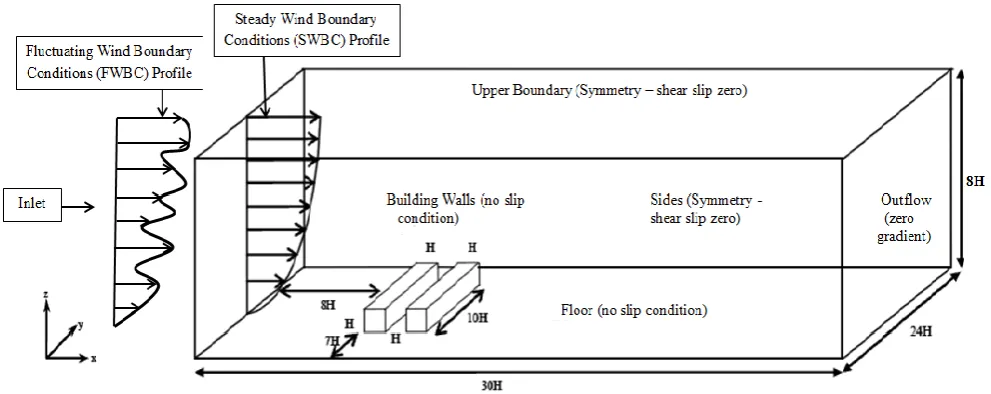
Fig. 1. Computational domain and boundary conditions for CFD simulation setup in ANSYS FLUENT

Fig. 2. (a) Velocity and (b) TKE profiles for the inlet boundary conditions showing similarity between CODASC profile [13] and

simulated UDF profiles 0

1 2 3 4 5

0 0.4 0.8 1.2 1.6

z/H

U/Uʜ Velocity Profile

CODASC Simulated UDF

0 1 2 3 4 5

0 0.5 1 1.5

z/H

TKE/TKEʜ Turbulent Kinetic Energy

Profile

CODASC Simulated UDF

the model is scaled by 1:150 similar to the wind tunnel experimental model. The computational domain is discretized using 1.2 million hexahedral elements integrating recommendations based on the wall y+ approach [14].

B. Boundary Conditions

An inlet and outlet boundary conditions are applied at the entrance and exit of the domain, respectively. Non-slip conditions are defined at the building walls and floors. To impose a parallel flow, symmetry conditions are indicated at the top and lateral sides of the computational domain [6]. Fig. 1 summarizes the computational domain and boundary conditions employed for the simulation.

In this study, CFD simulation is initially performed using a SWBC profile similar to that employed in the study by Salim et al. [6]. The inlet velocity profile is by a power law profile.

( ) ( ) (1)

The turbulent kinetic energy, k and dissipation rate, ε profiles are specified as

√ ( ) (2)

and

( ) (3)

with u being the vertical velocity profile, z being the vertical distance, δ being the boundary depth layer (≈ 0.5 m), being the friction velocity (= 0.54 m/s), being the von Kàrmàn constant (= 0.4) and lastly = 0.09. The similarity between the velocity and turbulent kinetic energy profiles from the UDF and CODASC are shown in Fig. 2

LES produces fluctuating profiles of flow variables at the outlet of the computational domain. The differences in the velocity profiles between SWBC and FWBC cases are illustrated in Fig. 3. It is observed that the profiles change

significantly with time and even the slightest temporal variation produces noticeable change.

Two approaches are employed in simulating results based on the generated FWBC. The first is through the use of

Fig. 3. Velocity profiles based on CODASC database [13], SWBC [6] and FWBC (at outlet)

0 1 2 3 4 5 6 7 8

0 1

z/H

U/Uʜ Velocity Profiles

CODASC Database

Simulated UDF (SWBC) FWBC at 5.0 second

0 1 2 3 4 5 6 7 8

0 1

z/H

U/Uн Velocity Profiles

FWBC at 3.0 second

FWBC at 6.0 second

FWBC at 8.0 second

FWBC at 14.0 second Proceedings of the World Congress on Engineering 2014 Vol II,

Fig. 4. Position of line sources from (a) computational domain (FLUENT), showing similarity with (b) wind tunnel setup (CODASC

database) [13]

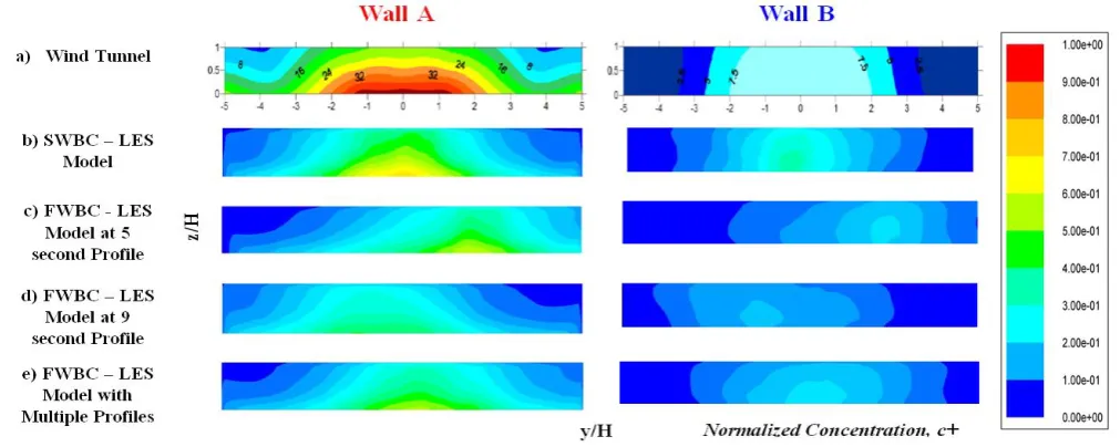
Fig. 5. Mean concentration contours on leeward (Wall A) and windward (Wall B) showing comparison between (a) WT data from CODASC database [13] (b) SWBC (c) FWBC at 5.0 second (d) FWBC at 9.0 second and (e) Multiple FWBC profiles

single fluctuating profile while the second approach involves applying multiple fluctuating profiles in the simulation. The different approaches implemented are summarized in Table 1 below:

TABLE 1.FLUCTUATING PROFILES USED IN SIMULATIONS

Simulations Fluctuating Profiles from Fig. 3 Simulation 1 5.0 second

Simulation 2 9.0 second

Simulation 3

0-10 second flow-time in ANSYS FLUENT = 3.0 second

10-20 second flow-time = 6.0 second 20-30 second flow-time = 8.0 second 30-40 second flow-time = 14.0 second

C. Flow Simulation

LES is employed for this study in order to account for both temporal and spatial fluctuations. The equations for continuity and momentum are:

̅̅̅

(4)

and ̅̅̅

̅ ̅̅̅

̅

̅̅̅

(5) The dynamic Smagorinsky-Lily sub-grid scale model is selected. Second order upwind discretization schemes are used for species and energy transport equations to increase the acccuracy and reduce numerical diffusion [15]. SIMPLEC and PRESTO! schemes are selected for the pressure-velocity coupling and pressure, respectively. The scaled residual criteria for all flow properties are set at 1 x 10-3. A dimensionless time-step of 0.0025 is chosen.

For the single fluctuating profiles simulations, 12000 time-steps are run to obtain approximately 40 flow-through times, translating to a physical time of 30 seconds.

For the multiple fluctuating profiles simulation, each profile is run for 4000 steps totalling to 16000 time-steps. This translates to a physical time of 40 seconds and

approximately 52 flow-through times. D. Dispersion Modeling

In order to replicate the pollutant source and traffic exhausts in this study, sulphur hexafluoride ( ) is used as tracer gas. The emission rate, Q is maintained at 10 g/s to replicate the study done by Salim et al. [6] and wind tunnel experiment from CODASC [13]. Line sources are used to model the release of the pollutant source and are achieved by separating sections of the volume in the geometry and defining them as different fluid zones. Their positions are illustrated in Fig. 4.

The advection-diffusion (AD) method is used for modeling the dispersion of pollutants species. In turbulent flows, this is computed as

( ) (6)

where D is the molecular diffusion coefficient for the pollutant in the mixture, is the turbulent eddy viscosity, Y is the mass fraction of the pollutant, ρ is the mixture density and is the turbulent Schmidt number.

Fig. 6. Velocity profiles along leeward wall (y/H = 0, y/H = 2.5 and y/H = -2.5) comparing between (a) SWBC (b) FWBC at 5.0 second (c) FWBC at 9.0 second and (d) Multiple FWBC profiles

(a) (b) (c) (d)

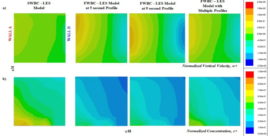
Fig 7. (a) Mean normalized vertical velocities, w and (b) mean normalized concentration contours, c+ at the mid-plane of the street canyon, comparing between SWBC, FWBC at 5.0 second, 9.0 second and multiple FWBC profiles

III. RESULTS AND DISCUSSIONS

Dispersion and distribution of the pollutants are observed through species concentration contours on the leeward (Wall A), windward (Wall B) as well as along the mid-plane within the street canyon.

Fig. 5 shows the results of mean concentration contours at Wall A and Wall B, comparing between FWBC, SWBC and WT. The numerical results clearly show the differences between SWBC and FWBC. SWBC with the LES model is shown to produce pollutant concentration distribution similar to WT, particularly in the vicinity of the centerline (y/H=0) at both Wall A and Wall B, underlining them as the most critical zone where maximum pollutant concentration occurs [6].

FWBC profiles showed variation from that of SWBC profiles. FWBC profiles with 5.0 and 9.0 second fluctuating profiles show pollutant concentration to be more prominent at the region to the right of the centerline (y/H ≈ 1.5) and to the left of the centerline (y/H ≈ 1.3), respectively. Besides, the results from multiple fluctuating profiles again show

pollutant concentration to be more prominent at the region to the right of the centerline (y/H ≈ 0.6). In addition, it can be observed that the magnitude of the pollutants predicted by the FWBC simulations are significantly lesser compared to the results under SWBC and WT. The variation in results can be explained through the velocity profiles obtained along the walls.

From Fig. 6 (a) it can be seen that the velocity profiles under SWBC along Wall A are consistently the same at all locations (y/H = 0, y/H = 2.5 and y/H = -2.5). While the velocity profiles for all the FWBC cases (i.e. Fig. 6 (b)-(d)) are fluctuating at both ends of Wall A. These differences in velocity cause pollutants concentrations to vary. The locations at which higher velocities occur indicate lower pollutant concentrations.

Predictions obtained from SWBC and FWBC profiles are compared in Fig. 7 based on the mean normalized vertical velocities and concentration contours along the mid-plane (y/H = 0) within the street canyon. It is observed that the spread of pollutants along the mid-plane between SWBC and all the FWBC simulations are similar with the only

1 2 3 4 5 6 7 8

0 1 2

z/H

U/Uн SWBC - Leeward

1 2 3 4 5 6 7 8

0 1 2

z/H

U/Uн FWBC 5.0s - Leeward

1 2 3 4 5 6 7 8

0 1 2

z/H

U/Uн FWBC 9.0s - Leeward

1 2 3 4 5 6 7 8

0 1 2

z/H

U/Uн

Multiple FWBC - Leeward

y/H = 0

y/H = 2.5

y/H = -2.5 Proceedings of the World Congress on Engineering 2014 Vol II,

Fig 8. Mean velocity magnitude contours across the computational domain for (a) SWBC (b) FWBC at 5.0 second (c) FWBC at 9.0

second and (d) Multiple FWBC profiles

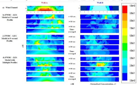
Fig. 9. Instantaneous normalized concentration data for (b) FWBC at 5.0 second (c) FWBC at 9.0 second and (d) Multiple FWBC profiles on Wall A and Wall B obtained with LES model compared to mean time-averaged data from (a) WT data from CODASC database [16]

notable difference being that SWBC produces higher magnitude of pollutants at the bottom left corner towards the leeward wall. The three FWBC simulations produce very high maximum magnitudes of positive and negative vertical velocities near both leeward and windward side of the canyon, prompting the pollutant concentrations to be lower near the bottom left corner of leeward wall as compared to SWBC.

Fig. 8 illustrates the velocity magnitude contours across the computational domain, comparing between SWBC and WBC profiles. For SWBC, the velocity contours produces consistent magnitude throughout the inlet side. Whereas, all

three FWBC simulations generated different magnitudes of velocities along the inlet side. The differences in the high velocity magnitude regions in all three FWBC cases inevitably caused the differences in pollutant concentration distribution in and around the street canyon region.

In actual situations, the pollutant dispersion may vary significantly in both time and space. Fig. 9 shows the instantaneous solutions of normalized concentration contours along Wall A and Wall B. The LES results of both SWBC and FWBC on both walls support the statement by Louka et al. [16], where time-evolution of concentration field illustrates significant variations in peak concentrations [6]. It further validates the results obtained from Fig. 5, showing similar pattern in terms of concentration contours. For example, it can be seen that for FWBC at 5.0 second, the pollutant concentrations are more prominent at the region to the right of the centerline for both walls. This is applicable to all the instantaneous solutions presented (t = 10 second, t = 20 second and t = 30 second). Similar trend is observed from the results of FWBC at 9.0 second whereby maximum pollutant concentrations occur at region to the left of the centerline.

IV. CONCLUSION

CFD simulations were performed to study air flow and pollutant dispersion in urban street canyons using LES. Two

implementing the more realistic FWBC in characterizing air flow and pollutant dispersion. It is imperative to consider the fluctuating component in wind velocity as real-time meteorological data are time dependent. The use of FWBC helps to provide more realistic predictions similar to real urban conditions.

In order to better predict the outcome of air flow and pollutant dispersion process, it is vital to take into account the temporal and spatial variations in the velocity profile. On top of that, WT testing could be replicated following fluctuating velocity profiles to obtain better experimental data for future validations based on meteorological data.

REFERENCES

[1] D. Schwela, “Air pollution and health in urban area,”Reviews on

Environmental Health, vol. 15, issue 1-2, pp. 13-42, 2011.

[2] R. Berkowicz, F. Palmgren, O. Hertel and E.Vignati, “Using measurements of air pollution in streets for evaluation of urban air quality – meteorological analysis and model calculations,”The

Science of the Total Environment 189/190, pp. 259-265, 1996.

[3] K. Ahmad, M. Khare and K. K. Chaudhry, “Wind tunnel simulation studies on dispersion at urban street canyons and intersections – a review,”Journal of Wind Engineering and Industrial Aerodynamics,

vol. 93, issue 9, pp. 697-717, 2005.

[4] A. M. Mfula, V.Kukadia, R. F. Griffiths and D. J. Hall, “Wind tunnel modeling of urban building exposure to outdoor pollution,”Atmospheric Environment, vol. 39, issue 15,pp. 2737-2745, 2005.

[5] N. Nikolopoulos, A. Nikolopoulos, I. Papadakis and K. –S. P. Nikas, “CFD Applications in Natural Ventilation of Buildings and Air Quality Dispersion,” CFD Applications in Energy and Environment

Sectors, vol. 1, pp. 53-100, 2011.

[6] S. M. Salim, A. Chan, R. Buccolieri and S. Di Sabatino, “Numerical simulation of atmospheric pollutant dispersion in an urban street canyon: Comparison between RANS and LES,”Journal of Wind

Engineering and Industrial Aerodynamics, vol. 99, pp. 103-113,

2011.

[7] R. E. Britter and S. R. Hanna, “Flow and dispersion in urban areas,”

Annual Review of Fluid Mechanics, vol. 35, pp. 1817-1831, 2003.

[8] Y. Tominaga and T. Stathopoulos, “CFD modeling of pollution dispersion in a street canyon: Comparison between LES and RANS,”Journal of Wind Engineering and Industrial Aerodynamics,

vol. 99, issue 4, pp. 340-348, 2011.

[9] C. Chang and R. Meroney, “Concentration and flow distributions in urban street canyons: wind tunnel and computational data,” Journal of

Wind Engineering and Industrial Aerodynamics, vol. 91, pp.

1141-1154, 2003.

[10] Y. W. Zhang, Z. L. Gu, Y. Cheng and S. C. Lee, “Effect of real-time boundary wind conditions on the air flow and pollutant dispersion in an urban street canyon – Large eddy simulations,” Atmospheric

Environment, vol. 45, pp. 3352-3359, 2011.

[11] C. Gromke and B. Ruck, “Influence of trees on the dispersion of pollutants in an urban street canyon – experimental investigations of the flow and concentration fields,” Atmospheric Environment, vol. 41,

pp. 3287-3302, 2007.

[12] C. Gromke and B. Ruck, “On the impact of trees on dispersion processes of traffic emissions in street canyons,” Boundary-Layer

Meteorology, vol. 131, pp. 19-34, 2009.

[13] CODASC, Concentration Data of Street Canyons, Laboratory of Building and Environmental Aerodynamics, IfH, Karlsruhe Institue of Technology, 2008.

[14] S. M. Salim, M. Ariff and S. C. Cheah, “Wall y+ _{approach for dealing}

with turbulent flows over a wall mounted cube,” Progress in

Computational Fluid Dynamics, vol. 10, pp. 1206-1211, 2010.

[15] H. K. Vesteeg and W. Malalasekera, An Introduction to

Computational Fluid Dynamics: The Finite Volume Method, Harlow,

Pearson Education Limited, 2007, ch. 5.

[16] P. Louka, S. E. Belcher and R. G. Harrison, “Coupling between air flow in streets and the well-developed boundary layer aloft,”

Atmospheric Environment, vol. 34, issue 16, pp. 2613-2621, 2000.