Parameter Estimation for Inventory of Load Models in Electric Power Systems

Parameter Estimation for Inventory of Load

Models in Electric Power Systems

Amit Patel, Kevin Wedeward, and Michael Smith

Abstract—This paper presents an approach to characterize power system loads through estimation of contributions from in-dividual load types. In contrast to methods that fit one aggregate model to observed load behavior, this approach estimates the inventory of separate components that compose the total power consumption. Common static and dynamic models are used to represent components of the load, and parameter estimation is used to determine the amount each load contributes to the cumulative consumption. Trajectory sensitivities form the basis of the parameter estimation algorithm and give insight into which parameters are well-conditioned for estimation. Parameters of interest are contributions to total load and initial conditions for dynamic loads. Results are presented for simulated data to demonstrate the feasibility of the approach.

Index Terms—electric power systems, load modeling, simu-lation, trajectory sensitivities, parameter estimation.

I. INTRODUCTION

As power system models and simulations used for plan-ning and stability studies become more advanced, higher fidelity models of all power system components are needed. Loads are particularly difficult to describe due to their diverse composition and variation in time, yet their importance to voltage stability and transient behavior has been recognized [1]–[4]. The approaches to load modeling can be catego-rized as either measurement-based or component-based [4]. Measurement-based approaches utilize data collected from a substation or feeder to develop a model that matches observed behavior (see, for example, [5]–[7]). Component-based approaches combine known models of all devices that make up the load (see, for example, [2], [4]). A combination of the approaches, known as identification of load inventory, has been developed where measurements are used to estimate the fraction (percentage) that each different device within a load contributes to the aggregate power consumed [8], [9].

The focus of this paper is development of a load inventory model where parameter estimation is used to determine the amount each component contributes to the total power consumption. Parameter estimation is achieved via a Gauss-Newton method based upon trajectory sensitivities (see [10]) which computes parameters that best fit simulated model responses to simulated measurements on a single phase. The results indicate which load contributions are well-conditioned for estimation and that those parameters can be accurately estimated in the presence of measurement error. Initial con-ditions of the dynamic states in the load models are difficult to identify; however, the load contribution coefficients are identifiable.

Manuscript submitted on July 13, 2014.

Amit Patel is with Accenture, Irving, TX 75039 USA.

Kevin Wedeward and Michael Smith are with the Institute for Complex Additive Systems Analysis (ICASA), New Mexico Institute of Mining and Technology, Socorro, NM 87801 USA, email: [email protected].

II. LOADMODELING

A wide variety of load models exist to mathematically represent the power consumed by a load and its dependencies on voltage, frequency, type and composition. Three common mathematical models for loads in power systems are pre-sented below and utilized in the proposed approach. In all cases, it is assumed that powers and voltages are normalized by base values such that their units are in per unit (p.u.) [11].

A. ZIP

A polynomial model is commonly used to represent loads and capture their voltage dependency. The average and reactive powers of the load are written as a sum of constant impedance (Z), constant current (I) and constant power (P), and referred to as the ZIP model [3], [11].

P = P0(K1p

V V0

2 +K2p

V

V0+K3p) (1)

Q = Q0(K1q

_V

V0

2 +K2q

V V0

+K3q) (2)

whereP, Q are the average and reactive power consumed by the load, respectively, P0, Q0 represent the nominal average and reactive power of the load, respectively,V is the magnitude of the sinusoidal voltage at the bus to which the load is connected,V0is the magnitude of the nominal voltage at the bus, and coefficientsK1p, K2p, K3p,K1q,K2q and

K3q define the proportion of each component of the model.

Coefficients for many load types have been experimentally determined and reported [2], [4], [5].

B. Exponential Recovery

The power profile is defined by

P = xp Tp

+P0

_V

V0

αt

(3)

Q = xq Tq

+Q0

_V

V0

βt

(4)

whereP, Q are the average and reactive power consumed by the load, respectively, P0, Q0 are the nominal average and reactive power, respectively,V is the magnitude of the sinusoidal voltage at the bus to which the load is connected, andV0 is the magnitude of the nominal voltage at the bus. Parameters Tp andTq are the average and reactive load

re-covery time constants, respectively,αsandβsare the

steady-state dependence of average and reactive powers on voltage, respectively, andαtand βt are the transient dependence of

and reactive power recovery, respectively, and are governed by the differential equations [7], [12], [13]:

˙ xp =

−xp

Tp

+P0

V V0

αs −

V V0

αt

(5)

˙ xq =

−xq

Tq

+Q0

_V

V0

βs −

_V

V0

βt! . (6)

Parameters for different load types have been experimentally determined and reported [7], [13].

C. Induction Motor

The induction motor’s voltages of interest are V ejθ ₌

V cos(θ) +jV sinθ at the stator terminal and V0ejθ0 ₌

v_d0 + jv_q0 at the voltage behind transient reactance. The

stator current is I = id + jiq = V e

jθ_−V0_ejθ0

Rs+jXs0 where X_s0 = Xs+ _XXrXm

r+Xm is the transient reactance. Additional parameters are stator resistance and leakage reactance, Rs

andXs, respectively, magnetizing reactance,Xm, and rotor

resistance and leakage reactance,Rr,Xr, respectively.

The voltage V0ejθ0 = v0_d+jv0_q has real and imaginary parts governed by the differential equations [11], [14]

dv0_d

dt = −

Rr

Xr+Xm

v0_d+

_X2

m

Xr+Xm

iq

+sv_q0(7)

dv_q0

dt = −

Rr

Xr+Xm

v0_q−

_X2

m

Xr+Xm

id

−sv_d0(8)

ds dt =

1 2H

Tmo(1−s)

2 −Te

(9)

where s = ωs−ωr

ωs is slip,ωr is rotor speed, ωs is angular velocity of the stator field, Tmo is a load torque constant,

Te = vd0id+vq0iq is electromagnetic torque, and H is the

motor and motor load inertia.

The average powerP and reactive powerQconsumed by the motor are then given by

P = Re(V ejθI∗)

= 1

R2

s+Xs02

Rs(V2+V cos(θ)vd0 −V sin(θ)v0q)

−X_s0(V cos(θ)v_q0 −V sin(θ)v_d0) (10)

Q = Im(V ejθI∗)

= 1

R2

s+Xs02

Rs(V cos(θ)vq0 −V sin(θ)vd0)

+Xs0(V2−V cos(θ)vd0 −Vsin(θ)v0q)

(11)

where(·)∗ denotes complex conjugate of the complex quan-tity, Re(·) and Im(·) denote the real and imaginary parts of a complex number, respectively. Parameters for different load types have been experimentally determined and reported [11], [15], [16].

D. Load Inventory Concept

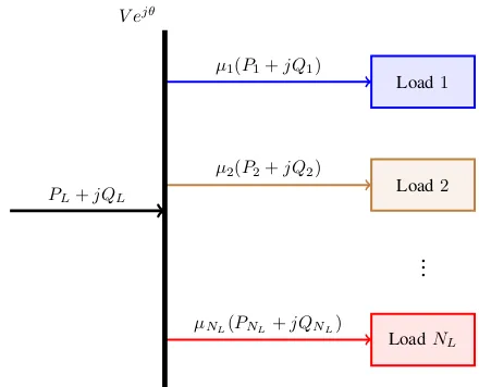
Load behavior will be modeled by using an aggregation of ZIP, exponential recovery and induction motor models from above with appropriate parameters selected for each to represent the load’s components. This is shown conceptually in Figure 1 with the total complex power consumedPL+jQL

the sum of the power consumed by all the individual load elements. The parameters of interest will be the contribution

Load1 µ1(P1+jQ1)

Load2 µ2(P2+jQ2)

...

LoadNL

µNL(PNL+jQNL)

V ejθ

[image:2.595.315.535.53.231.2]

PL+jQL

Fig. 1. Concept of load inventory

coefficientsµifori= 1,2, . . . , NLwhereNL is the number

of unique types of loads assumed to be connected to the bus as well as the initial conditions needed for each dynamic model.

In summary, the aggregate load with average power PL

and reactive power QL will be the fractional sum of each

individual type of model. Each model represents a candidate load that might exist in the inventory and its fractional contribution indicated by µi is the parameter of interest

for determining the inventory of loads. Total (aggregate) complex power is the sum of all load powers

PL+jQL = µ1(P1+jQ1) +µ2(P2+jQ2)

+· · ·+µNL(PNL+jQNL). (12)

III. TRAJECTORYSENSITIVITIES

Differential-algebraic models are often utilized to repre-sent the dynamic behavior of electric power systems [17]. When all loads are taken at a bus for the load inventory approach, the combined models presented above for loads can be represented in a manner similar to that of the broader power system:

˙

x = f(x, V) (13)

y = g(x, V, µ). (14)

Herexis the vector of dynamic states (e.g.,xp,xq, v0d,vq0,

s for dynamic loads) that satisfy the differential equations (13), y = [PL, QL]T is the 2×1 vector of total average

and reactive powers consumed by the aggregate load,V is the magnitude of the voltage at the bus (treated as an input) and µ is the vector of contributions µi=1,2,...,NL taken as parameters.

response of (13), (14) are defined as

x(t) = φx(λ, V, t) (15)

y(t) = g(φx(λ, V, t), λ, V, t) =φy(λ, V, t) (16)

wherex(t)satisfies (13), all parameters of interest are com-bined into the vectorλ= [x0, µ]T of dimensionM×1, and flows show the dependence of the trajectories on parameters λ(here initial conditions and fractional contributions), input V and time t. To obtain the sensitivity of the trajectories to small changes in the parameters ∆λ, a Taylor series expansion of (15), (16) can be formed. Neglecting higher order terms in the expansion yields

∆x(t) = φx(λ+ ∆λ, V, t)−φx(λ, V, t) (17)

≈ ∂φx(λ, V, t)

∂λ ∆λ≡xλ(t)∆λ (18) ∆y(t) = φy(λ+ ∆λ, V, t)−φy(λ, V, t) (19)

≈ ∂φy(λ, V, t)

∂λ ∆λ≡yλ(t)∆λ. (20)

The time-varying partial derivativesxλ andyλ are known as

the trajectory sensitivities, and can be obtained by differen-tiating (13) and (14) with respect to λ. This differentiation gives

˙

xλ = fx(t)xλ (21)

yλ = gx(t)xλ+gλ(t) (22)

where fx ≡ ∂f_∂x, gx ≡ ∂g_∂x and gλ ≡ ∂g_∂λ are time-varying

Jacobian matrices, and fλ ≡ ∂f_∂λ = 0. Along the trajectory

of the aggregate loads described by (13), (14) the trajectory sensitivities will evolve according to the linear, time-varying differential equations (21), (22). Initial conditions forxλ are

obtained from (15) by notingx(t0) =φx(λ, V, t0) =x0such that xλ(t0) =I whereI is the identity matrix [10]. Initial conditions foryλfollow directly from the algebraic equation

(22) to yieldyλ(t0) =gx(t0) +gλ(t0).

The N ×M sensitivity matrix for the ith output yi is now defined by taking sensitivities (22) at discrete times tk=0,1,...,N−1

Si(λj) = 

    

yi λ(t0)

yi λ(t1)

.. .

yi_λ(tN−1)



    

(23)

whereN is the number of discrete values of time at which values are taken from the trajectory sensitivity (22) found by numerically solving the coupled system (13), (14), (21), (22); M is the number of parameters inλ;λj _{is the particular set}

of values for parameters used when computing the trajectory and associated sensitivities; and for this particular application y1

λ = PLλ, y 2

λ = QLλ and the complete sensitivity matrix

S(λj) = "

S1_(λj₎

S2_(λj₎

#

is of dimension2N×M.

As an example of computing the equations that will be solved for trajectory sensitivities, assume the total power is given by (12) andP1,Q1are consumed by a load represented as the exponential recovery model’s powers (3), (4). The

sensitivities ofPL,QL to parameterµ1 are ∂PL

∂µ1 ≡PLµ1= P1= xp

Tp +P0

V V0

αt

(24)

∂QL

∂µ1 ≡QLµ1= Q1= xq

Tq +Q0

V V0

βt

(25)

where the statesxp,xq will come from numerical solution

of (5), (6) andV will be a specified input. The sensitivities ofPL,QL to the initial conditionsxp(0),xq(0)are

∂PL

∂xp(0)

≡PLxp(0) = µ1

1

Tp

∂xp

∂xp(0) =µ1

1

Tpxpxp(0) (26)

∂PL

∂xq(0)

≡PLxq(0) = 0 (27)

∂QL

∂xp(0)

≡QLxp(0) = 0 (28)

∂QL

∂xq(0)

≡QLxq(0) = µ1

1

Tq

∂xq

∂xq(0) =µ1

1

Tqxqxq(0) (29)

where the sensitivitiesxpxp(0) ≡ ∂xp

∂xp(0),xqxq(0) ≡ ∂xq

∂xq(0)will be the solution to the following differential equations that govern the trajectory sensitivities found by differentiating (5), (6) with respect to the initial conditionsxp(0),xq(0)

∂ ∂xp(0)

˙

xp≡x˙pxp(0) = −

1

Tp

∂xp

∂xp(0) =− 1

Tpxpxp(0) (30)

∂ ∂xq(0)

˙

xp≡x˙pxq(0) = 0 (31)

∂ ∂xp(0)

˙

xq ≡x˙qxp(0) = 0 (32)

∂ ∂xq(0)

˙

xq≡x˙qxq(0) = −

1

Tq

∂xq

∂xq(0) =− 1

Tqxqxq(0). (33)

Note the order of the derivatives (with respect to parameter and time) were interchanged in the process.

The differential equations (30), (33) that govern the trajec-tory sensitivities are solved numerically in parallel with the differential equations (5), (6) that govern the model such that trajectories are obtained for both. Calculations of sensitivities for all load models to all parameters are given in [18].

IV. PARAMETERESTIMATION

Parameter estimation will be cast as a nonlinear least squares problem and solved using a Gauss-Newton iterative procedure [17]. Measurements of average and reactive power consumed by a load during a disturbance will be used to estimate the unknown model parameters (here contributions and initial conditions). The aim of parameter estimation is to determine parameter values that achieve the closest match between the measured samples and the model’s simulated trajectory. Let measurements of the total average power PL and reactive power QL (denoted by PLm and QLm, respectively) consumed by the aggregate load be given by the appended sequences ofN measurements

~ ym=

"

[PLm(t0), PLm(t1), . . . , PLm(tN−1)]

T

[QLm(t0), QLm(t1), . . . , QLm(tN−1)]

T

#

(34)

with the corresponding simulated trajectory from numerically solving (13), (14) given by

~ y=

"

[PL(t0), PL(t1), . . . , PL(tN−1)]

T

[QL(t0), QL(t1), . . . , QL(tN−1)]

T

#

to get corresponding values at times tk=0,1,2,...,N−1. The mismatch between the measurements and corresponding model’s trajectory can be written in vector form as

~e(λ) =~y(λ)−~ym (36)

where the notation is used to show the dependence of the trajectory, and correspondingly the error, on the parameters λ. The vectors~e,~yandy~mwill be of dimension2N×1asN

measurements of PL andQL are assumed. The best match

between model and measurement is obtained by varying the parameters so as to minimize the error vector~e(λ)by some measure. One common measure is the two-norm (sum of squares) of the error vectors expressed as a cost function

C(λ) =1 2k~e(λ)k

2 2=

1 2

X2N−1

k=0 ek(λ)

2_{. (37)}

The errorek(λ)is thekth element of~eand can be linearly

approximated via a Taylor series expansion about an initial value ofλ=λj _{which yields}

ek(λ) ≈ ek(λj) +

∂ek(λj)

∂λ (λ−λ

j_{) (38)}

= ek(λj) +yλk(λ

j_{)∆λ (39)}

where ∂ek(λj)

∂λ = ∂yk(λj)

∂λ =yλk(λ

j_{)since the measurements}

ymk are independent ofλand the definition∆λ=λ−λ

j _is

utilized. The new value of λj denoted λj+1 will be chosen to minimize the following cost function with linearized error.

C(λ) = 1 2

X2N−1

k=0 (ek(λ

j_{) +y} λk(λ

j_)∆λ)2

= 1

2

X2N−1

k=0 (ek(λ

j_{) +S}

k(λj)∆λ)2

= 1

2

~e(λj) +S(λj)∆λ

2

2 (40)

whereSk is thekth row of the sensitivity matrixS.

Minimizing the cost function of linearized error (40) can now be performed via the Gauss-Newton method [17]. The process starts with an initial guess λ0 _{for parameter values} and then parameters are updated according to iterations of the following two steps.

S(λj)TS(λj)∆λj+1 = −S(λj)Te(λj) (41)

λj+1 = λj+αj+1∆λj+1 (42)

whereS is the trajectory sensitivity matrix defined in (23), αj+1 _{is a scalar that determines step size, and iterations stop} when ∆λj+1 _{is sufficiently small. The resulting parameter} values λj+1 _{will be a local minimum for the cost function} (37) due to the linearization and will be dependent on the initial guess λ0_{. An additional note is that the parameter} estimation process breaks down if ST_{S is ill-conditioned,}

i.e., nearly singular. This leads to the concept of identifia-bility and quantification of parametric effects [17], [19]. The invertibility of STS can be investigated through its singular values and condition number, eigenvalues, or magnitude of sensitivities over a trajectory via the 2-norm. The less-rigorous, 2-norm will be utilized here to gain insight into the condition of ST_{S. The 2-norm will be defined for the}

sensitivity of the ith output yi _{to the jth parameter λ} j

summed over discrete times tk as

Sij

2 2=

N−1

X

k=0

Sij(tk, λ)2. (43)

The size of the values computed via (43) will give an indication of the effect of parameters on the trajectory, and in turn give guidance as to which parameters can be estimated.

V. EXAMPLE OFAPPLICATION VIASIMULATION

The parameter estimation approach described above was implemented through simulation to estimate load contribu-tions and initial condicontribu-tions. Five loads, each represented by one of five models, were taken as connected to a bus as shown in Figure 1 with magnitude V of the bus’s phasor voltage taken to be the input to the models, and average and reactive powers PL, QL, respectively, taken to be the

(measurable) outputs. Load 1 was an exponential recovery model, load 2 was the model of a residential induction motor, load 3 was a model of a small industrial induction motor, load 4 was a model of a large industrial induction motor, and load 5 was a ZIP model. That made theM = 16 unknown parameters

λ =

xp1(0), xq1(0), v0d2(0), v0q2(0), s2(0), v0d3(0), v0q3(0),

s3(0), v0_d4(0), v_q0₄(0), s4(0), µ1, µ2, µ3, µ4, µ5 T (44)

which includes initial conditions for all the states in the individual models as well as the fractional contributions of each load model to the aggregate power consumed. For the five loads considered, the total load is given by

PL+jQL = µ1(P1+jQ1) +µ2(P2+jQ2)

+µ3(P3+jQ3) +µ4(P4+jQ4)

+µ5(P5+jQ5) (45)

with NL = 5; µi=1,2,...,5 the fractional contributions of each load model;P1, Q1 given by (3), (4);P2, Q2 given by (10), (11);P3, Q3 given by (10), (11);P4, Q4given by (10), (11); andP5, Q5given by (1), (2). Representative values for parameters used in each model were taken from [4], [13], [16] and are given in Table I, and the nominal bus voltage is taken to beV0= 1p.u.

TABLE I

PARAMETER VALUES FOR MODELS OF LOADS

Load Model and Parameters 1 Exponential Recovery

P0 TP αs αt Q0 Tq βs βt

1.25 60 0 2 0.5 60 0 2

2 Induction Motor - Residential

Rs Xs Xm Rr Xr H T0

0.077 0.107 2.22 0.079 0.098 0.74 0.46 3 Induction Motor - Small Industrial

Rs Xs Xm Rr Xr H T0

0.031 0.1 3.2 0.018 0.18 0.7 0.6 4 Induction Motor - Large Industrial

Rs Xs Xm Rr Xr H T0

0.013 0.067 3.8 0.009 0.17 1.5 0.8 5 ZIP

P0 K1p K2p K3p Q0 K1q K2q K3q

1.0 0.15 0.6 0.25 0.7 0.05 -0.05 1.0

A. Results when no error in measurements

was dropped from its nominal value of 1p.u. to 0.97p.u. at 50 seconds. With the initial conditions and load contributions at specified values, the simulation was run to generate synthetic, “measured” data to represent data that might be collected by a voltage disturbance monitor or phasor measurement unit. A sampling rate of 10Hz was used to record the total average and reactive powers consumed by the five loads. Nominal values for parameters are given in Table II, and plots of the aggregate power consumptionPLandQLare given in Figure

2 as the solid lines.

The simulation was then modified to run with initial guesses for parameter values, and the iterative Gauss-Newton process described by (41), (42) implemented to update the values of the parameters until they converged to within a specified tolerance. At each iteration, the system’s model (13), (14) and trajectory sensitivities (21), (22) were nu-merically solved using Matlab’s ode15s() solver for a new trajectory using updated values of the parameters. The results of the iterative process can be seen Figure 3 and show convergence of the load contributions to values used to create the synthetic measurements. The final, estimated values of all parameters (both initial conditions and load contributions) are given in Table II. The simulated trajectories forPL andQL

as the parameters are updated can be seen as the dashed lines in Figure 2.

TABLE II

VALUES,GUESSES AND ESTIMATES OF PARAMETERS

Load Model and Estimated Parameters 1 Exponential Recovery

xp(0) xq(0) µ1

value: 0.0010 0.0007 0.1000 guess: 0.0025 0.0015 0.3000 estimate: 0.0010 0.0007 0.1000 2 Induction Motor - Residential

v_d0(0) v0q(0) s(0) µ2

value: 0.8659 0.1439 0.0399 0.2000 guess: 0.9000 0.1800 0.0550 0.3000 estimate: 0.8659 0.1439 0.0399 0.2001 3 Induction Motor - Small Industrial

v0

d(0) v 0

q(0) s(0) µ3

value: 0.8842 0.0527 0.0120 0.2000 guess: 0.9000 0.0750 0.0600 0.1000 estimate: 0.8840 0.0527 0.0121 0.2001 4 Induction Motor - Large Industrial

v_d0(0) v0q(0) s(0) µ4

value: 0.9124 0.0308 0.0078 0.3000 guess: 0.8900 0.5000 0.0150 0.2000 estimate: 0.9125 0.0308 0.0078 0.2999 5 ZIP

µ5

value: 0.2000

guess: 0.1000

estimate: 0.2000

B. Study of identifiability

[image:5.595.307.544.54.153.2]

For the sample application above where no measurement error was introduced, the 2-norm of all sensitivities was calculated and shown in Table III. Of particular note is that the sensitivities of the average and reactive power are at least an order of magnitude larger for load contributions than

Fig. 2. Average power (left) and reactive power (right) consumed by aggregate load; simulated measurements are solid lines and trajectories for updated parameter estimates are dashed lines

Fig. 3. Estimates of parameters (as markers/symbols) representing load contributions over iterations; dashed lines are actual values

initial conditions. This indicates that the load contributions have a larger impact on the trajectory and in turn should be more readily identified through parameter estimation. When no measurement error was assumed, both initial conditions and load contributions were identified, but when random error was introduced (as discussed in the next section) the estimates of the initial conditions were inaccurate. The zero entries in the table imply that the load models’ powers do not depend on that particular parameter.

As an additional check of identifiability for the parameters of interest, both the condition number and eigenvalues were computed for the matrix ST_{S. The condition number was}

[image:5.595.319.537.206.506.2]

TABLE III

2-NORM OF TRAJECTORY SENSITIVITIES FOR PARAMETERS(LOAD

CONTRIBUTIONS AND INITIAL CONDITIONS)OF INTEREST

Load Model and 2-norm of Trajectory Sensitivities 1 Exponential Recovery

xp(0) xq(0) µ1

kSPLk

2

2: 0.029 0 7.920

kSQLk

2

2: 0 0.027 15.37

2 Induction Motor - Residential v0

d(0) v 0

q(0) s(0) µ2

kSPLk

2

2: 0.005 0.003 0.002 14.37

kSQLk

2

2: 0.002 0.001 0.001 13.59 3 Induction Motor - Small Industrial

v0

d(0) v 0

q(0) s(0) µ3

kSPLk

2

2: 0.001 0.003 0.002 1.116

kSQLk

2

2: 0.081 0.003 0.008 3.220 4 Induction Motor - Large Industrial

v0

d(0) v 0

q(0) s(0) µ4

kSPLk

2

2: 0.004 0.003 0.003 4.095

kSQLk

2

2: 0.009 0.005 0.007 4.725 5 ZIP

µ5

kSPLk

2

2: 75.97

kSQLk

2

2: 64.89

small eigenvalues were associated with the initial conditions and much larger eigenvalues were associated with the load contributions.

C. Results with 2% random error in measurements

The study described above was repeated, but this time with an error in each measurement achieved by adding a normally distributed random number to each measurement with mean 0 and standard deviation 2%. The method of estimating parameters worked well for the load contributions, but not the initial conditions. This is attributed to the issues with identifiability discussed above. Table IV shows the “true values”, initial guesses and estimates of the parameters representing load contributions in this case.

TABLE IV

VALUES,GUESSES AND ESTIMATES OF PARAMETERS WHEN2%

RANDOM ERROR IN MEASUREMENTS

Load Model and Estimated Parameters 1 Exponential Recovery

µ1 value guess estimate 0.1000 0.3000 0.1231 2 Induction Motor - Residential

µ2 value guess estimate 0.2000 0.3000 0.1698 3 Induction Motor - Small Industrial

µ3 value guess estimate 0.2000 0.1000 0.1740 4 Induction Motor - Large Industrial

µ4 value guess estimate 0.3000 0.2000 0.3102 5 ZIP

µ5 value guess estimate 0.2000 0.1000 0.2272

VI. CONCLUSION

This paper presented an application of trajectory sensitivi-ties and parameter estimation to estimate an aggregate load’s composition. An example is presented using simulated data for five types of loads modeled by an exponential recovery model, three induction motor models with different param-eters, and a ZIP model. Future work will be to incorporate and investigate additional models, and apply the approach to real data collected from a voltage disturbance monitor or phasor measurement unit.

REFERENCES

[1] A. Ellis, D. Kosterev, and A. Meklin, “Dynamic load models: Where are we?” in Proceedings of the IEEE Power Engineering Society Transmission and Distribution Conference, May 2006.

[2] D. Kosterev, A. Meklin, J. Undrill, B. Lesieutre, W. Price, D. Chassin, R. Bravo, and S. Yang, “Load modeling in power system studies: WECC progress update,” inProceedings of the IEEE Power and En-ergy Society General Meeting - Conversion and Delivery of Electrical Energy in the 21st Century, July 2008.

[3] IEEE Task Force on Load Representation for Dynamic Performance, “Load representation for dynamic performance analysis [of power systems],” IEEE Transactions on Power Systems, vol. 8, no. 2, pp. 472–482, May 1993.

[4] W. Price, K. Wirgau, A. Murdoch, J. V. Mitsche, E. Vaahedi, and M. El-Kady, “Load modeling for power flow and transient stability computer studies,”IEEE Transactions on Power Systems, vol. 3, no. 1, pp. 180–187, Feb 1988.

[5] A. Bokhari, A. Alkan, R. Dogan, M. Diaz-Aguilo, F. de Leon, D. Czarkowski, Z. Zabar, L. Birenbaum, A. Noel, and R. Uosef, “Experimental determination of the ZIP coefficients for modern res-idential, commercial, and industrial loads,” IEEE Transactions on Power Delivery, vol. 29, no. 3, pp. 1372–1381, June 2014.

[6] D. Han, J. Ma, R.-m. He, and Z.-Y. Dong, “A real application of measurement-based load modeling in large-scale power grids and its validation,”IEEE Transactions on Power Systems, vol. 24, no. 4, pp. 1756–1764, Nov 2009.

[7] D. Karlsson and D. J. Hill, “Modelling and identification of nonlinear dynamic loads in power systems,” IEEE Transactions on Power Systems, vol. 9, no. 1, pp. 157–166, February 1994.

[8] D. R. Sagi, S. J. Ranade, and A. Ellis, “Evaluation of a load composition estimation method using synthetic data,” inProceedings of the 37th Annual North American Power Symposium, October 2005. [9] S. Ranade, D. Sagi, and A. Ellis, “Identifying load inventory from measurements,” inProceedings of the IEEE Power and Energy Society Transmission and Distribution Conference and Exhibition, May 2006. [10] I. A. Hiskens and M. A. Pai, “Power system applications of trajectory sensitivities,” inProceedings of the Power Engineering Society Winter Meeting, 2002.

[11] P. Kundur,Power system stability and control, N. J. Balu and M. G. Lauby, Eds. McGraw-Hill, Inc., 1994.

[12] D. J. Hill, “Nonlinear dynamic load models with recovery for voltage stability studies,”IEEE Transactions on Power Systems, vol. 8, no. 1, pp. 166–176, Feb 1993.

[13] I. R. Navarro, “Dynamic load models for power systems - estimation of time-varying parameters during normal operation,” PhD thesis, Lund University, Lund, Sweden, September 2002.

[14] A. Ellis, “Advanced load modeling in power systems,” PhD thesis, New Mexico State University, Las Cruces, NM, December 2000. [15] F. Nozari, M. Kankam, and W. Price, “Aggregation of induction motors

for transient stability load modeling,”IEEE Transactions on Power Systems, vol. 2, no. 4, pp. 1096–1103, Nov 1987.

[16] IEEE Task Force on Load Representation for Dynamic Performance, “Standard load models for power flow and dynamic performance simulation,”IEEE Transactions on Power Systems, vol. 10, no. 3, pp. 1302–1313, Aug 1995.

[17] I. A. Hiskens, “Nonlinear dynamic model evaluation from disturbance measurements,”IEEE Transactions on Power Systems, vol. 16, no. 4, pp. 702–710, November 2001.

[18] A. Patel, “Parameter estimation for load inventory models in electric power systems,” MS thesis, New Mexico Institute of Mining and Technology, Socorro, NM, December 2008.